Transitions to Nematic states in homogeneous suspensions of high aspect ratio magnetic rods

Gopinath A.‡, Mahadevan L.‡, and Armstrong R. C ‡Division of Engineering and Applied Sciences, Harvard University, Cambridge, MA 02138
§Department of Chemical Engineering, MIT, Cambridge, MA 02139.
Abstract

Isotropic-Nematic and Nematic-Nematic transitions from a homogeneous base state of a suspension of high aspect ratio, rod-like magnetic particles are studied for both Maier-Saupe and the Onsager excluded volume potentials. A combination of classical linear stability and asymptotic analyses provides insight into possible nematic states emanating from both the isotropic and nematic non-polarized equilibrium states. Local analytical results close to critical points in conjunction with global numerical results (Bhandar, 2002) yields a unified picture of the bifurcation diagram and provides a convenient base state to study effects of external orienting fields.

Recently, a kinetic theory based model for dispersions of acicular magnetic particles was developed1,2 using ideas grounded in classical models for liquid-crystalline polymers3. Effects of Brownian motion, anisotropic hydrodynamic drag, a steric force chosen to be of the Maier - Saupe form and a mean-field magnetic potential were included. Both continuum descriptions obtained via closure approximations and the diffusion equation were solved numerically for some parameter ranges1,2. The focus of this article is on obtaining a theoretical characterization of transitions to nematic states from a homogeneous base state of a suspension of slender high aspect ratio magnetic particles. Combining local asymptotic and stability analysis near critical points with global numerical results, we obtain a physically convenient point of departure for investigations of external aligning fields. Both the Maier-Saupe and the Onsager potentials are considered. Results for the Maier-Saupe potential are in excellent agreement with available numerical solutions of the equations and complement recent investigations on the classical Doi model4.

The particles in the homogeneous dispersion are modeled as two point masses connected by a rigid massless rod of length L and diameter $d$ with inherent magnetic dipoles, the magnetic moment being along the axis1,2. We envisage a situation in which $d$ and $L$ are kept constant and the concentration of the rods can be varied. The orientation of the rod is specified by the unit vector $\bf u$ along the axis from one specified bead to another. In the mean-field approximation it suffices to consider one test particle in a sea of others. Denoting the orientation distribution function by $f({\bf u},t)$, one writes for the case of constant diffusivity in scaled form6

$${\partial{f}\over\partial{t}}=\Re_{\bf u}\boldsymbol{\cdot}(\Re_{\bf u}f+f\Re_{\bf u}(V_{EV}+V_{M})).$$ (1)

Here $\Re_{{\bf u}}(.)$ is the rotation operator and the potentials are measured in units of $k_{b}T$. We define the average of a quantity, ${\bf X}({\bf u})$, as $\langle{\bf X}({\bf u})\rangle\equiv\int{\bf X}({\bf u})\>f({\bf u})d{\bf u}$. The excluded volume intermolecular potential for a Maier-Saupe (MS) or Onsager (O) potential can then be written as

$$V_{EV}({\bf u})=\int\beta_{MS/O}({\bf u},{\bf u}^{\prime})\>f({\bf u}^{\prime},t)\>d{\bf u}^{\prime},$$ (2)

where, $\beta_{MS}({\bf u},{\bf u}^{\prime})=-\Pi_{MS}({\bf u}\cdot{\bf u}^{\prime})^{2}$, $\Pi_{MS}$ being a phenomenological constant proportional to the concentration of rods, $N$ and $\beta_{O}({\bf u},{\bf u}^{\prime})=2NL^{2}d\>|{\bf u}\times{\bf u}^{\prime}|$. The total potential due to the mean magnetic field, $V_{M}$, can be written2

$$V_{M}=-{(3/2)}\mathcal{B}^{\prime}\langle{\bf u}{\bf u}\rangle:{\bf u}{\bf u}-\mathcal{A}^{\prime}{\bf u}\boldsymbol{\cdot}\langle{\bf u}\rangle+{\mathcal{A}}_{o}+{\mathcal{B}}_{o}$$ (3)

The first term reflects a net magnetic interaction potential due to average order1,2, the second term is the mean field approximation to the dipole-dipole interaction between particles and ${\mathcal{A}}_{o}$ and ${\mathcal{B}}_{o}$ are constants independent of ${\bf u}$.

Equations (1)-(3) do not involve any preferred direction for orientation of possible nematic states and so we choose to employ an expansion for $f({\bf u},t)$ in terms of spherical harmonic functions $Y_{l}^{m}({\bf u})=Y^{m}_{l}(\theta,\phi)$. where ${\bf u}=(\sin{\theta}\sin{\phi})\>{\bf e}_{x}+(\sin{\theta}\cos{\phi})\>{\bf e}_{y}+(\cos{\theta})\>{\bf e}_{z}$ and ${\bf e}_{z}$ is the axis from which $\theta$ is measured. Since $f$ is real valued, we can write

$$f({\bf u},t)=\sum_{l=0}^{\infty}\sum_{m=-l}^{+l}b_{l}^{m}(t)Y_{l}^{m}({\bf u}),$$ (4)

where $b_{l}^{-m}(t)=(-1)^{m}\overline{b_{l}^{m}(t)}$ for all $m\geq 0$ (the over-bar denotes complex conjugation) and $b^{0}_{0}=(4\pi)^{-1/2}$ $\forall$ $t$ due to the normalization condition. Nematic states with fore-aft symmetry satisfy $f({\bf u})=f(-{\bf u})$, and for these $l$ is restricted to the set of even integers. The macroscopic state of the suspension can be quantified by three variables - the structure tensor, ${\bf S}\equiv\langle{\bf u}{\bf u}\rangle-{\mbox{\boldmath$\delta$}}/3$, the concomitant scalar structure factor $S_{e}\equiv 9({\bf S}\boldsymbol{\cdot}{\bf S}\boldsymbol{\cdot}{\bf S})/2]^{1/3}$ and the mean polarity ${\bf J}\equiv\langle{\bf u}\rangle$. We now specify the two inner products, $\langle Y^{m}_{l}|f\rangle\equiv\int\overline{Y_{l}^{m}({\bf u})}\>f({\bf u},t)\>d{\bf u}$, and $\langle l_{1},m_{1}|l_{2},m_{2}|l_{3},m_{3}\rangle\equiv\int\overline{Y_{l_{1}}^{m_{1}}({\bf u})}\>Y_{l_{2}}^{m_{2}}({\bf u})\>Y^{m_{3}}_{l_{3}}({\bf u})\>d{\bf u}$ and functions $d_{2n}=[\pi(4n+1)(2n-3)!!(2n-1)!!][2^{(2n+2)}n!(n+1)!]^{-1}$ and $c_{o}(l^{\prime})=[(l^{\prime}-1){(l^{\prime}-3)!!}^{2}][(l^{\prime}+2){(l^{\prime}!!)}^{2}]^{-1}.$

Using these definitions with (4) we can write (2) as

$$V_{MS}=-{3\over 2}U({8\pi\over 15})\sum_{l^{\prime}=0}^{\infty}\sum_{m^{\prime}=-l^{\prime}}^{l^{\prime}}\delta_{l^{\prime},2}Y_{l^{\prime}}^{m^{\prime}}({\bf u})b_{l^{\prime}}^{m^{\prime}},$$ (5)

and

$$V_{O}=-4\pi U\sum_{l^{\prime}=1}^{\infty}\sum_{m^{\prime}=-2l^{\prime}}^{+2l^{\prime}}{d_{2l^{\prime}}\over(4l^{\prime}+1)}Y_{2l^{\prime}}^{m^{\prime}}({\bf u})b_{2l^{\prime}}^{m^{\prime}}$$ (6)

with $U=2NL^{2}d$. In writing (5) and (6) we have ignored constants linear in $U$ and independent of ${\bf u}$. The expressions are the same as those for non-magnetizable rods because the excluded volume potential is just dependent on geometrical symmetries. Parameters $\mathcal{A}^{\prime}$ and $\mathcal{B}^{\prime}$ in (3) are proportional to the number density of the particles, and can be rewritten as $\mathcal{A}^{\prime}=\mathcal{A}U$ and $\mathcal{B}^{\prime}=\mathcal{B}U$. Henceforth $U$, $\mathcal{A}$ and $\mathcal{B}$ are treated as three independent parameters. Combining (1), (4), (5) and (6) and using appropriate inner products we get the following evolution equation for the modes $b_{l}^{m}$,

$${d{b_{l}^{m}}\over dt}=-l(l+1)\>b_{l}^{m}-\sum_{p=0}^{\infty}\sum_{q=-p}^{+p}(\sigma_{EV}+\sigma_{M}),$$ (7)

where

$$\sigma_{M}={4\pi U}\sum_{l^{\prime}=0}^{\infty}\sum_{m^{\prime}=-l^{\prime}}^{+l^{\prime}}b_{p}^{q}b_{l^{\prime}}^{m^{\prime}}({{\mathcal{B}\delta_{l^{\prime},2}}\over 5}+{{\mathcal{A}\delta_{l^{\prime},1}}\over 3})\Psi$$ (8)

and $\sigma_{EV}$ depends on the nature of the excluded volume potential,

$$\sigma_{MS}={{4\pi U}\over 5}\sum_{l^{\prime}=0}^{\infty}\sum_{m^{\prime}=-l^{\prime}}^{+l^{\prime}}b_{p}^{q}b_{l^{\prime}}^{m^{\prime}}\delta_{l^{\prime},2}\Psi,$$ (9)
$$\sigma_{O}={4\pi U}\sum_{l^{\prime}=0}^{\infty}\sum_{m^{\prime}=-2l^{\prime}}^{+2l^{\prime}}{d_{2l^{\prime}}\over 4l^{\prime}+1}b_{p}^{q}b_{l^{\prime}}^{m^{\prime}}\Psi.$$ (10)

The function $\Psi=\Psi(l,m,p,q,l^{\prime},m^{\prime})$ is given by

$$\Psi(l,m,p,q,l^{\prime},m^{\prime})=-mm^{\prime}\langle l,m|p,q|l^{\prime},m^{\prime}\rangle$$
$$-{1\over 2}({{[l(l+1)-m(m+1)]\over{[l^{\prime}(l^{\prime}+1)-m^{\prime}(m^{\prime}+1)]^{-1}}}})^{1\over 2}\langle l,m+1|p,q|l^{\prime},m^{\prime}+1\rangle$$
$$-{1\over 2}({{[l(l+1)-m(m-1)]\over{[l^{\prime}(l^{\prime}+1)-m^{\prime}(m^{\prime}-1)]^{-1}}}})^{1\over 2}\langle l,m-1|p,q|l^{\prime},m^{\prime}-1\rangle$$ (11)

It is clear from equations (7)-(11) that nematic branches corresponding to $(\mathcal{A}=0$, $\mathcal{B}\geq 0)$ and thus $J=0$ form a subset of possible stationary solutions to (7). It is also clear that $(S=0,J\neq 0)$ states are un-physical.

A linear stability analysis of (7) about the isotropic state, fo(𝐮)=(4π)1subscript𝑓𝑜𝐮superscript4𝜋1f_{o}({\bf{u}})=(4\pi)^{-1} is readily performed using blm=(blm)o+ϵblm+O(ϵ2)superscriptsubscript𝑏𝑙𝑚subscriptsuperscriptsubscript𝑏𝑙𝑚𝑜italic-ϵsuperscriptsubscript𝑏𝑙superscript𝑚𝑂superscriptitalic-ϵ2b_{l}^{m}=(b_{l}^{m})_{o}+\epsilon{b}_{l}^{{}^{\prime}m}+O(\epsilon^{2}), ϵ1much-less-thanitalic-ϵ1\epsilon\ll 1 being a suitable amplitude, and retaining terms through O(ϵ)𝑂italic-ϵO(\epsilon). The growth rates or eigenvalues, λlmsuperscriptsubscript𝜆𝑙𝑚\lambda_{l}^{m}, corresponding to the disturbance Ylm(𝐮)superscriptsubscript𝑌𝑙𝑚𝐮Y_{l}^{m}({\bf u}) can be obtained from the linearized equations. For the Maier-Saupe potential we get the following eigenvalues (for odd and even l𝑙l respectively) (λlm)MS=l(l+1)(1δl,1𝒜U/3)subscriptsuperscriptsubscript𝜆𝑙𝑚𝑀𝑆𝑙𝑙11subscript𝛿𝑙1𝒜𝑈3(\lambda_{l}^{m})_{MS}=-l(l+1)(1-\delta_{l,1}\mathcal{A}U/3), and (λlm)MS=l(l+1)(1U(1+)δl,2/5)subscriptsuperscriptsubscript𝜆𝑙𝑚𝑀𝑆𝑙𝑙11𝑈1subscript𝛿𝑙25(\lambda_{l}^{m})_{MS}=-l(l+1)(1-U(1+\mathcal{B})\delta_{l,2}/5), indicating that there are two critical points on the S=0𝑆0S=0 isotropic branch. The first critical point satisfies (1+)Uca=51superscriptsubscript𝑈𝑐𝑎5(1+\mathcal{B})U_{c}^{a}=5. The critical eigenvalue is five fold degenerate with the associated destabilizing eigenvectors being linear combinations of Y2msuperscriptsubscript𝑌2𝑚Y_{2}^{m}, m=2,1,0,1,2𝑚21012m=-2,-1,0,1,2. The second critical point satisfies Ucb=3𝒜1superscriptsubscript𝑈𝑐𝑏3superscript𝒜1U_{c}^{b}=3\mathcal{A}^{-1} and the critical eigenvalues that change sign at this point are three-fold degenerate and
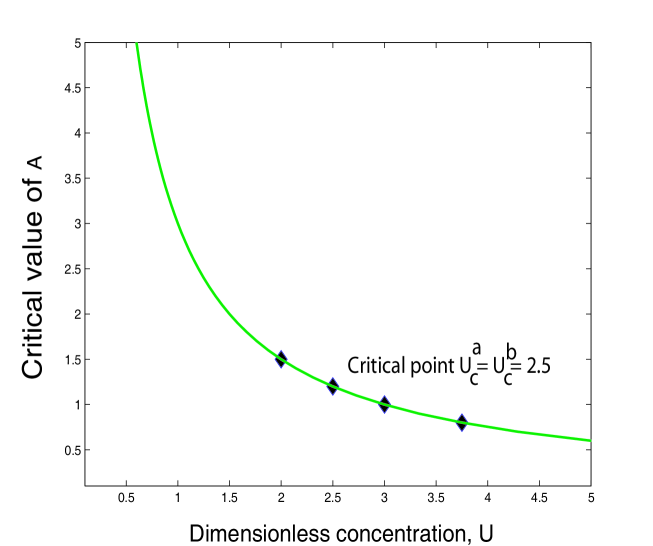
 correspond to the eigenvectors Y1msuperscriptsubscript𝑌1𝑚Y_{1}^{m}, m=1,0,1𝑚101m=-1,0,1. In Figure (1) we plot these analytical predictions and compare them to numerically obtained solutionsBhandar for the case =11\mathcal{B}=1. We note that for fixed and finite \mathcal{B}, as 𝒜𝒜\mathcal{A}\rightarrow\infty, Ucb0superscriptsubscript𝑈𝑐𝑏0U_{c}^{b}\rightarrow 0. As 𝒜𝒜\mathcal{A} decreases from very large values, Ucb<Ucasuperscriptsubscript𝑈𝑐𝑏superscriptsubscript𝑈𝑐𝑎U_{c}^{b}<U_{c}^{a} initially and then, beyond a critical value of 𝒜𝒜\mathcal{A}, we get Ucb>Ucasuperscriptsubscript𝑈𝑐𝑏superscriptsubscript𝑈𝑐𝑎U_{c}^{b}>U_{c}^{a}. For =11\mathcal{B}=1, the two critical points coincide for 𝒜=1.2𝒜1.2\mathcal{A}=1.2. Detailed numerical calculations show that for Ucb<Ucasuperscriptsubscript𝑈𝑐𝑏superscriptsubscript𝑈𝑐𝑎U_{c}^{b}<U_{c}^{a}, the branch is prolate, otherwise it is an oblate branch. For the Onsager potential we find (for odd and even l𝑙l respectively) (λlm)O=l(l+1)(1𝒜Uδl,1/3)subscriptsuperscriptsubscript𝜆𝑙𝑚𝑂𝑙𝑙11𝒜𝑈subscript𝛿𝑙13{(\lambda_{l}^{m})_{O}}=-l(l+1)(1-\mathcal{A}U\delta_{l,1}/3), and (λlm)O=l(l+1)(1U(1+)δk,1/5+Uπco(l)/2)subscriptsuperscriptsubscript𝜆𝑙𝑚𝑂𝑙𝑙11𝑈1subscript𝛿𝑘15𝑈𝜋subscript𝑐𝑜𝑙2{(\lambda_{l}^{m})_{O}}=-l(l+1)(1-U(1+\mathcal{B})\delta_{k,1}/5+U\pi c_{o}(l)/2). Thus for odd l𝑙l, as for the Maier-Saupe potential, there is one critical point on the S=0𝑆0S=0 line, Ucbsuperscriptsubscript𝑈𝑐𝑏U_{c}^{b}, which is the same as before. The destabilizing eigenvectors are the 333 independent components of Y1m(𝐮)superscriptsubscript𝑌1𝑚𝐮Y_{1}^{m}({\bf u}). Let us denote the critical points for even l𝑙l by Uca(l)superscriptsubscript𝑈𝑐𝑎𝑙U_{c}^{a}(l) such that the critical eigenvectors at each point are the 2l+12𝑙12l+1 independent components of Ylm(𝐮)superscriptsubscript𝑌𝑙𝑚𝐮Y_{l}^{m}({\bf u}). The first critical point occurs at Uca(2)=(πco(2)/2+/5)1superscriptsubscript𝑈𝑐𝑎2superscript𝜋subscript𝑐𝑜2251U_{c}^{a}(2)=(\pi c_{o}(2)/2+\mathcal{B}/5)^{-1} and corresponds to the eigenvector set Y2m(𝐮)superscriptsubscript𝑌2𝑚𝐮Y_{2}^{m}({\bf u}). Higher order bifurcations occur at Ucb(l)=2(πco(l))1superscriptsubscript𝑈𝑐𝑏𝑙2superscript𝜋subscript𝑐𝑜𝑙1U_{c}^{b}(l)=2(\pi c_{o}(l))^{-1} for l4𝑙4l\geq 4 (k=2,3,..)(k=2,3,..).

We now concentrate on bifurcations of $J>0$ branches from the non-trivial $J=0$ nematic states for the specific case of a Maier-Saupe inter-molecular potential. As a point of departure to frame our discussion, we focus on the vicinity of the critical concentration given by $U_{c}^{a}=U_{c}^{b}$ and study the bifurcating branches as $\mathcal{A}$ and $U$ are varied with $\mathcal{B}$ held fixed.

Since the equations (1), (3), (7), (8) and (9) with $\mathcal{A}=0$ exhibit rotational symmetry, we consider a base nematic state of the form (3) with coefficients $(b_{l}^{m})_{o}$ real and non-zero only if both $l$ and $m$ are even. From (1), (3) and (8) it is clear that the potential $U$ and the parameter $\mathcal{B}$ can be combined into one dimensionless factor, $W=U(1+\mathcal{B})$. Consider a base nematic state with director ${\bf n}={\bf e}_{z}$ such that $\cos{\theta}=({\bf u}\boldsymbol{\cdot}{\bf n})$. Then the steady, uniaxial solution for this nematic is given by $f(\theta)={\exp{(3WS_{e}\cos{2\theta}/4)}}/P$, where $P$ is a normalizing constant. This yields

$${{2S_{e}+1}\over 3}=(\int_{0}^{1}\exp{({3\over 2}WS_{e}t^{2})}t^{2}dt)(\int_{0}^{1}\exp{({3\over 2}WS_{e}t^{2})}dt)^{-1}$$

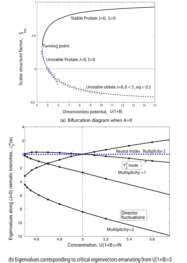
plotted in Figure (2a). The solid lines are linearly stable branches. The oblate phase where the rods are oriented randomly in the $({\mbox{\boldmath$\delta$}}-{\bf n}{\bf n})$ plane, is unstable to director fluctuations but stable if these are artificially suppressed - this is exemplified by the open circles which denote solutions obtained in integrating (1) in time in the subspace mentioned above4. Brownian dynamics simulations of the system for the Maier-Saupe potential5 and $\mathcal{B}_{m}=0$ indicate that results using time integration for short times can yield an apparently stable oblate phase, thus mimicking for short times the effect of a pinned director. However long time integration of the stochastic system leads to the oblate branch being destabilized by symmetry breaking perturbations. We expect similar considerations to hold for ${\mathcal{B}}\geq 0$.

For later analysis we need an expression for the solution curve close to the critical point $W=5$. An regular perturbation expansion in the small parameter, $\hat{W}\equiv W-5$ indicates that along the nematic branches, we have the approximate relationship

$$S_{e}(\hat{W})\approx-{7\over 25}{\hat{W}^{\prime}}+{119\over 625}{\hat{W}}^{{}^{\prime}2}-{29981\over 171875}{\hat{W}}^{{}^{\prime}3}+O(\hat{W}^{{}^{\prime}4}),$$ (12)

also plotted in Figure (2a) as the dash-dot line. We expect this to be accurate close to the critical point only. The structure factor for this nematic state has the form ${\bf S}_{o}=-S_{e}(W){\bf S}^{(1)}/3$, with $(S^{(1)}_{xx}=S^{(1)}_{yy}=-S^{(1)}_{zz}/2)$. The eigenvalues obtained from (7) corresponding to the destabilizing eigenvectors, $Y_{2}^{m}$, are shown in Figure (2b). There are five eigenvalues that are zero at $U_{c}^{a}$. The one corresponding to $Y_{2}^{0}$ (the structure parameter mode) has multiplicity of $1$. The other four correspond to director fluctuations and occur as two pairs, one of which is identically zero. Since there are two independent ways to rotate a director on a sphere, we expect two neutral eigen-directions.

We now impose small perturbations to the base state, $b_{l}^{{}^{\prime}m}$, comprised only of even $m$ modes while $l$ can be both even and odd. The equation for the growth of mode $b_{1}^{{}^{\prime}0}$ with $\Psi_{(1)}=\Psi(1,0,2,0,1,0)=1/\sqrt{(5\pi)}$ and $\Psi_{(2)}=\Psi(1,0,1,0,2,0)=-3/\sqrt{(5\pi)}$ is:

$${d{b_{1}^{{}^{\prime}0}}\over dt}=-2\>b_{1}^{{}^{\prime}0}(1-{U\mathcal{A}\over 3}+{{2\pi U\mathcal{A}}\over 3}(b_{2}^{0})_{o}\Psi_{(1)}$$
$$-{{4\pi U}\over{5(1+\mathcal{B})}}\sum_{p=0}^{\infty}\sum_{q=-p}^{+p}\sum_{m^{\prime}=-2}^{2}b_{p}^{{}^{\prime}q}(b_{2}^{m^{\prime}})_{o}\Psi(1,0,p,q,2,m^{\prime}))$$ (13)

Close to criticality, the $b_{1}^{{}^{\prime}0}$ mode dominates and so the $p=3$ term in (13) can be ignored to leading order. Setting the growth rate to zero yields the following equation for $\mathcal{A}^{c}(\mathcal{B},U)$ valid for small $S_{e}$,

$$[1+{2\pi\over 5}(1+\mathcal{B})U(b_{2}^{0})_{o}\Psi_{(2)}]={U\mathcal{A}^{c}\over 3}(1-2\pi(b_{2}^{0})_{o}\Psi_{(1)}).$$ (14)

To obtain local information about the nature of the $J>0$ branches close to the critical point $U_{c}^{a}=U_{c}^{b}$, we expand all quantities in terms of a small parameter $\delta$ that denotes the distance from the critical point measured along the $(J=0)$ nematic branches - to obtain (a) $U=5(1+\mathcal{B})^{-1}(1+\delta\hat{U})$, (b) $\mathcal{A}^{c}=3(1+\mathcal{B})(1+\delta\hat{\mathcal{A}}^{c})/5$ and (c) $(b_{2}^{0})_{o}=\delta(\hat{b_{2}^{0}})_{o}\approx\delta U^{\prime}(d/d\hat{U})_{0}(\hat{b_{2}^{0}})_{o}=\delta k_{m}\hat{U}$ with the slope $k_{m}=-7\sqrt{5}(10\sqrt{\pi})^{-1}$. Substituting these expressions in (14) yields at $O(\delta)$

$$\hat{\mathcal{A}}^{c}=(2\pi(\Psi_{(1)}+\Psi_{(2)})k_{m}-1)\hat{U}={9\over 5}\hat{U}$$ (15)

Thus, close to the critical point as as we move along the prolate (with $\hat{U}$ locally decreasing), $\hat{\mathcal{A}}^{c}$ decreases as well. Similarly, as one moves along the oblate towards more higher values of $U$ ($\hat{U}$ increases), $\hat{\mathcal{A}}^{c}$ increases. In short, critical points on the $(J=0$, $S_{e}<0)$ oblate state have $\mathcal{A}^{c}>1.2$ and on the $(J=0$, $S_{e}>0)$ prolate state satisfy $\mathcal{A}^{c}<1.2$.

Our analysis yields insight about the behavior close to the critical point. Crucially, we find that it accords with numerical solutions far from the critical point obtained by Bhandar1 for the specific case =11\mathcal{B}=1. Combining our local analytic results with these global numerical results, we obtain 
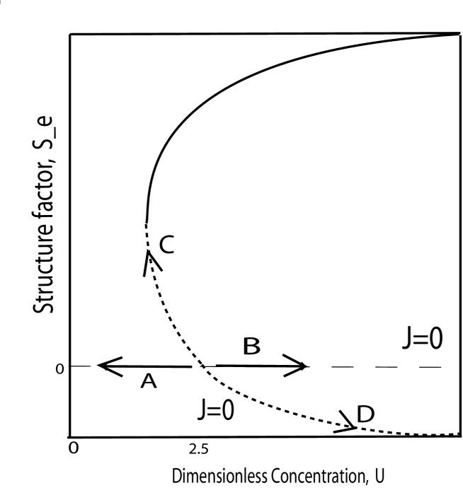
the bifurcation scenario illustrated in Figure 3. Let us recast the results in terms of the dependence of 𝒜csuperscript𝒜𝑐\mathcal{A}^{c} on the scalar structure parameter. For a fixed value of 𝒜𝒜\mathcal{A}, there are two critical points at which the J=0𝐽0J=0 branch becomes unstable to disturbances comprised of Y10superscriptsubscript𝑌10Y_{1}^{0} components. One of them is always on the Se=0subscript𝑆𝑒0S_{e}=0 isotropic branch and the other is always on the (Se0,J=0)formulae-sequencesubscript𝑆𝑒0𝐽0(S_{e}\neq 0,J=0) nematic solution. When 𝒜<1.2𝒜1.2\mathcal{A}<1.2, the J>0𝐽0J>0 branches bifurcate at one point in the segment (Se=0(S_{e}=0, U>5/2)U>5/2) and at one point in the the prolate branch (J=0(J=0 , Se>0subscript𝑆𝑒0S_{e}>0. Even though the J=0𝐽0J=0 nematic prolate has a turning point at U2.245𝑈2.245U\approx 2.245, the salient qualitative results of the local analysis holds even far from the critical point.

Consider now the effects of an imposed external magnetic field ${\bf H}$ modeled by adding a term to the potential to (1) and (3) that is proportional to ${\bf u}\boldsymbol{\cdot}{\bf H}$. Such a field breaks the rotational degeneracy of the system inherent in (1). We anticipate that for a fixed values of $U$, $\mathcal{A}$ and $\mathcal{B}$, the degree of order $S$ as well as the extent of average polarization $J$ change continuously with $H$. The transition from an isotropic to nematic state is replaced by a transition from a weakly aligned (paranematic) state to a strongly aligned state. Our results provide a mathematically convenient and physically relevant starting point to investigate these scenarios.

Acknowledgements

AG thanks Dr. Bhandar for providing a copy of the dissertation from which the simulation data used for comparison (in Figure 1) was obtained.

References

  • (1) A. S. Bhandar, A constitutive theory for magnetic dispersions, PhD Dissertation, The University of Alabama (2002).
  • (2) A. S. Bhandar, and J. M. Weist, Mesoscale constitutive modeling of magnetic dispersions, J. Colloid Interface Sci., 257, 371 (2003).
  • (3) R. G. Larson and H.  C. Öttinger, Orientation distribution function for rod-like polymers, Macromolecules, 24, 6270 (1991).
  • (4) A. Gopinath, R. C. Armstrong and R. A. Brown, Observations on the eigenspectrum of the linearized Doi equation and application to numerical simulations of liquid crystal suspensions, J. Chem. Physics, 121 (12), 6093 (2004).
  • (5) C. I. Siettos, M. D. Graham and I. G. Kevrekidis, Coarse Brownian dynamics for nematic liquid crystals: Bifurcation, projective integration, and control via stochastic simulation, J. Chem. Phys., 118(22), 10149 (2003).
  • (6) The assumption of constant diffusivity is reasonable as we are concerned only with equilibrium nematic states.
Refer to caption
Figure 1: A plot of the analytical value of $\mathcal{A}(U)$ for the Maier-Saupe potential at which the instability to $Y_{1}^{m},$ $m=-1,0,1$ modes arises on the isotropic $J=S=0$ branch. The circles are re-normalized computed results obtained from a numerical solution for $\mathcal{B}=1$ from Bhandar (2002)1.
Refer to caption
Figure 2: (a) The equilibrium bifurcation diagram of the base nematic states with $J=0$ for $\mathcal{A}=0$. The prolate branch arising from $U_{c}^{a}$ is unstable to structure factor fluctuations but regains stability beyond the turning point. The dash-dot line is the curve corresponding to the asymptotic expansion (12). (b) The eigenvalues corresponding to the destabilizing eigenvectors $Y_{2}^{m}$ at $U_{c}^{a}$ when $\mathcal{A}=0$. The turning point is at $W=U(1+\mathcal{B})\approx 4.49$
Refer to caption
Figure 3: Schematic sketch of the bifurcation scenario obtained by a combination of our local analytical results and global numerical results for $\mathcal{B}=1$. Region (A) corresponds to $0<U<U_{c}^{a}$, $S_{e}=J=0$ and $\infty<\mathcal{A}^{c}<1.2$. As $U$ increases, the critical value of $\mathcal{A}$ decreases, reaching $1.2$ at $U=U_{c}^{a}=5(1+\mathcal{B})^{-1}$. Region (B) corresponds to $U_{c}^{a}<U<\infty$, $S_{e}=J=0$ and $1.2<\mathcal{A}^{c}<0$. Region (C) denotes bifurcation of $(J>0$, $S_{e}>0)$ nematic branches from the $(J=0$, $S_{e}>0)$ prolate curve. In this region, as one moves to $S_{e}\rightarrow 1$, $\mathcal{A}^{c}$ decreases from 1.2 to 0. Finally in region (D) along the oblate branch with $(J=0$, $S_{e}<0)$, we find $\mathcal{A}^{c}$ increasing from 1.2 as $S_{e}$ decreases from 00 to $-1/2$.