Numerical Study of the Oscillatory Convergence to the Attractor at the Edge of Chaos.

Abstract

This paper compares three different types of “onset of chaos” in the logistic and generalized logistic map: the Feigenbaum attractor at the end of the period doubling bifurcations; the tangent bifurcation at the border of the period three window; the transition to chaos in the generalized logistic with inflection 1/2 ($x_{n+1}=\mu x_{n}^{1/2}$), in which the main bifurcation cascade, as well as the bifurcations generated by the periodic windows in the chaotic region, collapse in a single point. The occupation number and the Tsallis entropy are studied. The different regimes of convergence to the attractor, starting from two kinds of far-from-equilibrium initial conditions, are distinguished by the presence or absence of log-log oscillations, by different power-law scalings and by a gap in the saturation levels. We show that the escort distribution implicit in the Tsallis entropy may tune the log-log oscillations or the crossover times.

I Introduction

The transition from regular to chaotic regime presents characteristics similar to phase transitions in statistical thermodynamics and an adequate statistical thermo-dynamical formalism has been developed for chaotic systems (see ref. beck for an introduction). The transition point, or border of chaos, is characterized by a null Lyapunov exponent. The interesting features of this transition were first illustrated by the pioneering works of Feigenbaum on the logistic map attractor at the infinite bifurcation point feig , immediately followed by a series of theoretical works grass81 , politi , mori . In these investigations a power-law behavior of the sensitivity function of the logistic map at the threshold of chaos was formulated and the values for the power-law exponent were analytically calculated. More recently Tsallis Ts:88 introduced a formalism of non-extensive thermodynamics that allows to pass easily from the chaotic case to the null Lyapunov exponent case, recovering the Boltzmann Gibbs (BG) formulation as a limit. This formalism enlightens the connections between chaos and border of chaos and, in particular, defines a generalized entropy as the quantity of physical interest. For example it has been shown An:04 that a strong analogy with the Pesin Identity Pesin exists among this generalized entropy and generalized polynomial sensitivity to initial conditions appropriate to describe the sensitivity at the infinite bifurcations point of the logistic map Ba:02 .

Also other statistical formalisms emerging within special relativity kaniadakis and quantum groups abe seem to describe well noi the analogies between the threshold of chaos and the fully chaotic regime, even if recently the non-extensive formalism has been strongly criticized grass2005 revealing a still open debate on the subject. At this time a lot of experimental results (see Ts:rev for a review) seem to confirm at least part of the theoretical framework of the non-extensive formalism. In this paper we performed various numerical experiments devoted to investigate the logistic map at transition points presenting different routes to chaos. Thus our study regards different border of chaos regimes with different attractors underlying the dynamics. We present a joint analysis of (generalized, coarse grained) entropy and occupation number. We investigate the dynamics at large times and at large sampling ratios and analyze border of chaos transitions different from the Feigenbaum attractor in the logistic map. Finally we examine the presence of oscillations in the convergence to the attractor.

II Numerical experiments on the Feigenbaum attractor

In this paper we describe a set of numerical experiments, performed on the logistic map at the onset of chaos, with the purpose of examining the dynamics of a statistical ensemble of points, starting from far-from-equilibrium initial conditions. In each experiment the available phase space is partitioned in a number W_box of elementary, equal cells. A set of N points is randomly selected in the phase space according to two kinds of initial set-ups, and iterated according to the map. In these experiments we used the logistic map in the form

$$x_{i+1}=1-\mu x_{i}^{2}\;\;;\;\;\;\;-1\leq x\leq 1\;\;;\;\;\;\;0\leq\mu\leq 2~{}.$$ (1)

We investigated the parameter values $\mu$ = 2 for the fully chaotic case, $\mu_{\infty}$ = 1.401155189.. at the Feigenbaum attractor, $\mu_{tg}$ = 1.75 at the tangent bifurcation and $\mu_{1/2}$ = 2/$\sqrt{3}$ when the logistic is generalized with inflection 1/2 ($x_{i+1}=1-\mu x_{i}^{1/2}$). The first kind of initial start-up is from concentrated initial conditions (i. c.). All the N points are chosen, with a uniform random distribution, inside a single cell of the partition, itself chosen at random. In the second kind of experiment all the N initial points are uniformly and randomly distributed in all the available phase space (spread i. c.). The i-th cell will contain a fraction N_i/N of the total number of points ($\sum_{i=1}^{W_{box}}N_{i}=N$), so that one can naively define a probability of occupation for the i-th cell through $p_{i}=N_{i}/N$ with the constraint $\sum_{i=1}^{W_{box}}p_{i}=1$. On one hand we observe, for both kinds of experiments (concentrated and spread i. c.) the occupation number in time, namely the number of non empty cells of the partition. On the other hand, the other quantity of interest in our discussion is the physical entropy, defined as coarse-grained entropy through the probabilities $p_{i}$. We will use the Tsallis definition of entropy Ts:88 , useful to characterize the behavior at the onset of chaos where the Lyapunov exponent vanishes:

$$S_{q}^{TS}=\frac{1-\sum_{i=1}^{W_{box}}p_{i}^{q}}{q-1}$$ (2)

Other definitions of entropies kaniadakis ; abe ; noi would also work for the purposes of this paper. The analysis is performed through comparisons of the various behaviors between chaotic regime and border of chaos. We use different partitions W_box and different sampling ratios r, defined as $r$=N/W_box, that gives an indication of the goodness of sampling.

The fact that the Lyapunov exponent is zero at the threshold of chaos, allows us to use power-laws to characterize the evolution grass81 ; politi ; Ts:97 ; Ly:98 . The comparison with the chaotic case makes natural to pass from an ”exponential formalism” to an ”extended exponential formalism” describing the power-law An:04 ; Ka:04 . As discussed in La:99 , in the Chaotic regime, the (averaged) time evolution of the map, starting from concentrated initial conditions, may happen in two or three stages: a first “thermalization” stage heavily dependent on the details of the initial conditions; a second “linear” stage in which the coarse grained Boltzmann-Gibbs (BG) entropy $S_{BG}$ grows linearly with time and a third “saturation” stage in which $S_{BG}$ reaches its final equilibrium value.

In the fully chaotic regime, when proper average is made on different experiments of the same kind (see ref. La:00 ), the evolution of the logistic map, starting from concentrated initial conditions (CIC), exhibits an initial exponential growth of the occupation number without a first thermalization stage. A saturation is reached, depending on the grid size, when N_occ equals the fractal support value (N_occ = W_box for $\mu$ = 2). The coarse grained version of the BG entropy shows a linear initial increase followed by a saturation at a S${}_{BG_{sat}}$ level (S${}_{BG_{sat}}\simeq\ln(W_{box})$) when starting from CIC. A Pesin-like identity can be observed for the coarse-grained BG entropy. Using for this case a non-extensive formalism La:00 ; Ba:01 ; An:04 ; noi , a linear growth of S_q in the first evolution stage can be found and a Pesin-like identity can be recovered, if the appropriate entropic index is selected . Thus some features of the chaotic case can be directly transferred to the threshold of chaos. It is important to note that in the chaotic case the evolution happens in only two stages. In this paper we are interested in clarify how the final saturation stage is reached at the onset of chaos. To this aim we studied the evolution at longer times than the previous works. The results are illustrated in Figs.1 and 2, where, differently from the chaotic case, we can observe roughly three stages. The first stage is the analogue of the chaotic one: both $\langle N_{occ}\rangle$ and $\langle S_{q}\rangle$ increase and reach a maximum. The duration of this first stage becomes longer and the maximum level higher increasing W_box, while they do not depend on $r$. As previously stressed An:04 ; noi ; La:00 , in this first “linear” stage, $\langle S_{q}\rangle$ grows linearly only for the proper entropic index ($q=0.36$ when $\mu=\mu_{\infty}$). In the second stage both $\langle N_{occ}\rangle$ and $\langle S_{q}\rangle$ decrease. $\langle N_{occ}\rangle$ follows a power-law with superimposed log-log oscillations which amplitude increases with $r$ and does not depend on W_box. For low enough $q$ values, $\langle S_{q}\rangle$ reproduces the $\langle N_{occ}\rangle$ behavior (when $q\simeq 0\;$ results $S_{q}\simeq N_{occ}-1$), but the amplitude of oscillations decreases with increasing $q$ and vanishes when $q\sim 0.36$ (see fig.2 right frame). In the third stage $\langle N_{occ}\rangle$ and $\langle S_{q}\rangle$ reach their (W_box dependent) saturation values and the evolution ends. Note that the saturation is reached at a level that increases with W_box, but $\langle N_{occ}\rangle$ results in a lower final value than the fractal support, that is equal to $N_{occ}=244$ (799) for W${}_{box}=10^{4}$ ($10^{5}$).

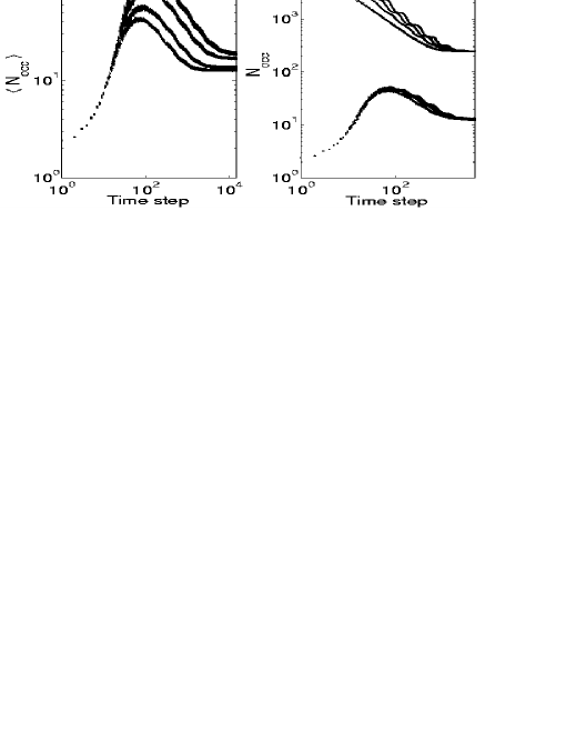
Figure 1: (a): time evolution of the average occupation number $\langle N_{occ}\rangle$ for the Logistic map at $\mu_{\infty}$. Different curves correspond to different W_box with $r$=1 (from top to bottom $W_{box}=10^{5},5\cdot 10^{4},2\cdot 10^{4},10^{4}$).
(b): N_occ vs. time from spread initial conditions (upper curves) and $\langle N_{occ}\rangle$ from CIC (lower curves). Fixed W_box (10⁴) and different $r$ (from top to bottom: $r$= 1000,100,10,1 upper curves, $r$= 100, 10, 1 lower curves). The averages are made over 5000 randomly chosen initial configurations.

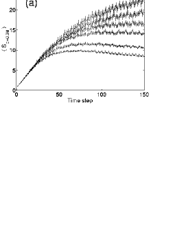
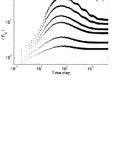
Figure 2: Logistic map at the critical point $\mu=1.401155189$. Tsallis Entropy $\langle S_{q}\rangle$ is averaged over $N_{av}=5000$ random choices of an expansion experiment initial cell and is plotted together its statistical error. (a): different point ensembles are relative to increasing $W_{box}$ values (from top to bottom $W_{box}=5\cdot 10^{5},2\cdot 10^{5},10^{5},5\cdot 10^{4},2\cdot 10^{4},10^{4}$) while the entropic index $q=0.36$ (the value that linearize the first evolution stage) and the sampling ratio $r=1$ do not vary. (b): fixed $W_{box}=10^{4}$ and $r=100$, the point ensembles are relative to different entropic indexes (from top to bottom $q=0.001,0.1,0.2445,0.36,0.7,1$).

The log-log oscillations of N_occ have been already observed in the logistic map at $\mu=\mu_{\infty}$ Mo:00 ; To:05 , performing numerical experiments starting from uniform i. c. (see fig.1 -b). Here, for the first time, we can observe this same behavior for $\langle N_{occ}\rangle$ starting from CIC (see fig.1 -b). This kind of logarithmic oscillations, superimposed to a power-law, characterize a large number of systems exhibiting discrete scale invariance sornette . The time evolution $N_{occ}(t)=t^{-\delta}\,P(\ln(t))$ (where $P(\ln(t))$ is a periodic function) can be expanded in Fourier series and, keeping only the first term, can be written in the form:

$$N_{occ}(t)\,=\,t^{-\delta}\,A\left(1\,+\,B\cos(\omega\ln(t)+\phi)\right)$$ (3)

As can be observed in fig.1-b (upper curves), starting from uniform i. c., the exponent $\delta$ increases with $r$ (this dependence has been stressed in To:05 ) and its limit value ($\delta\rightarrow 0.800138...$ for $r\rightarrow\infty$) has been determined in grass2005 . We analyzed the results of our experiments from concentrated i. c., using for $\langle N_{occ}\rangle(t)$ the same time dependence of eq.(3), founding the power-law exponent $\delta\simeq 0.54$, but we could not establish any dependence on $r$. Note that also starting from uniform i. c. the evolution can be roughly divided into three stages: a first “crossover time” stage, in which $N_{occ}(t)\simeq$const. ; the power-law stage, with superimposed log-log oscillations; the final saturation stage, in which $N_{occ}(t)$ equals the fractal support value, differently to the CIC experiments.

To investigate the origin of the observed behavior (on average) starting from CIC, we performed others expansion experiments, without averaging, selecting a special initial cell. In fig.3 we show the results of an expansion experiment from the $W_{box}$-th cell, that has the point $x=1$ as right extreme, where the distance of $x=1$ from the Feigenbaum attractor is infinitesimal. Again there are three evolution stages. The first stage presents, for both $N_{occ}(t)$ and $S_{q}$, exactly the same pattern already observed for the sensitivity function starting from $x_{0}=1$, characterized by large fluctuations mori . The upper limit values correspond to times $n=2^{k}-1$ and form a straight line for $N_{occ}(t)$ and $S_{q=0.2445}$ as already found for the sensitivity function Ba:02 . This stage is longer when $W_{box}$ increases. In the second stage, the upper limit of the large fluctuation pattern decreases, following approximately a power-law with superimposed log-log oscillations. Finally a saturation stage is reached, in which the evolution shows a regular periodic pattern. Some features of the evolution from this special cell remind the averaged behavior. This is not trivial because there are single cells which exhibit a completely different time evolution. We checked, for instance, the repellor $x=x_{r}=0.5602326...$ (solution of the equation $x_{r}=1-\mu_{\infty}x_{r}^{2}$). Centering the initial cell in $x_{r}$, we observed a first stage in which $N_{occ}$ grows exponentially and reaches its maximum at $N_{occ}\sim W_{box}$; then it decreases following a power-law without log-log oscillations and its evolution ends at a saturation value equal to the fractal support. Large fluctuations of $N_{occ}$ and $S_{q}$ do not appear at any time.

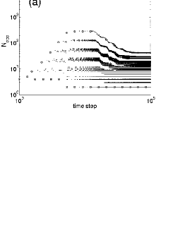
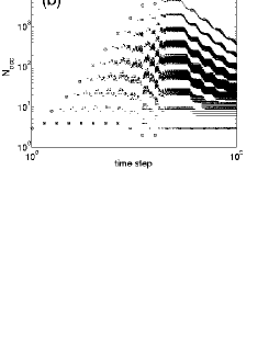
Figure 3: Time evolution of the Logistic map at the critical point $\mu=1.401155189$, the maximum values are reached at time $n=2^{k}-1$ (with $k=1,2,3,...$) and are stressed by circles, minimum in $2^{k}$ by squares. $N_{occ}$ vs. time obtained by an expansion experiment starting from an initial condition concentrated in the extremely right cell (centered in $x_{c}=1-1/(2W_{box})$), sampling ratio $r=1$, number of partition cells $W_{box}=10^{5}$ in (a) and $W_{box}=10^{7}$ in (b).

The Feigenbaum-scaling cascade of period doubling is not the only possible scenario. In the following we show few comparisons with others routes to chaos. The logistic map at the beginning of the period three window ($\mu=\mu_{t}=7/4$) exhibit both a vanishing Lyapunov exponent ($\lambda=0$) and a power-law decreasing sensitivity function (weak insensitivity). The power-law exponent and the correspondent $S_{q}$ entropic index ($q=3/2$) have been analytically determined in Ba:02_2 . We performed for the tangent point $\mu=\mu_{t}$ the same relaxation experiments described in the previous part for $\mu=\mu_{\infty}$, reproducing and improving the results already obtained in Co:04 and To:04 . Our results are showed in fig.4. As already stressed in Co:04 , the evolution starting from CIC begins miming a chaotic behavior: $S_{BG}$ grows linearly and $\langle N_{occ}\rangle$ exponentially; then a maximum is reached. Thereafter $\langle N_{occ}\rangle$ presents a “crossover” stage, with $\langle N_{occ}\rangle=const.\sim W_{box}$, which is longer for larger $r$. This has been already analyzed in To:04 for uniform i. c. but not for CIC. In the third stage $\langle N_{occ}\rangle$ decreases with a power-law and no log-log oscillations. The evolution ends when $\langle N_{occ}\rangle$ reaches the three points attractor. The curves relatives to CIC and to uniform i. c. join each other after the first stage (fig. 4 -a), differently from the $\mu=\mu_{\infty}$ case (fig.1 -b). Turning our attention to fig. 4-b $S_{q}$, after the mimed “chaotic” stage, decreases and is linear only for $q$ = 3/2. There is no crossover time for any sampling ratio and for $q$ = 3/2 the slope depends on $W_{box}$ Co:04 but not on $r$.

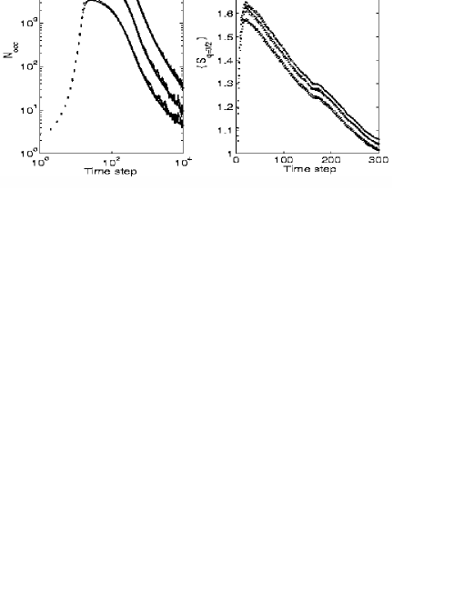
Figure 4: Logistic map at the tangent point $\mu=\mu_{t}$. $W_{box}=10^{4}$, averages performed using $N_{av}$=800 random choices for the initial cell. (a): $N_{occ}$ from a relaxation experiment starting from uniform i. c. (continuous lines) and $\langle N_{occ}\rangle$ obtained starting by a CIC (points), are plotted together for different $r$ values (from top to bottom $r=1,10,100$). (b): Tsallis entropy with index $q=3/2$ is showed for different $r$ (top to bottom $r=1,10,100$); the three series of points are inside their statistical errors (not showed in figure).

Finally we examined the transition to chaos in the generalized logistic map when the inflection is 1/2. Here the main bifurcation cascade, as well as the bifurcations generated by the periodic windows in the chaotic region, collapse in a single point inflection . In such a point the map undergoes the transition to chaos and the Lyapunov exponent is zero. The experiments performed starting from uniformly spread i. c. show again two features already encountered in the previous cases. There exists a “crossover time ” (fig.5) which is more extended for larger $r$. Thereafter it appears a regime of convergence to the attractor in which N_occ follows a power-law with negative exponent and no log-log oscillations. In the limits of our numerical experiments such exponent depends neither on the grid nor on the sampling ratio.

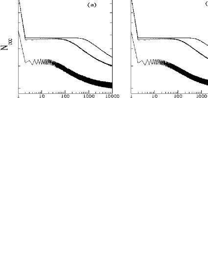
Figure 5: Evolution from spread i. c. at $\mu_{1/2}$ in the generalized logistic with inflection 1/2. The curves are obtained, from top to bottom, using $r$ = 100, 10, 1 for $W_{box}$ = 64.000 (a) and $W_{box}$ = 128.000 (b).

III Conclusions

Our numerical experiments show that the long time evolution on the Feigenbaum attractor from CIC happens in three stages, instead of the two observed in the chaotic case. The saturation is reached only after a power law decreasing stage, with superimposed log-log oscillations, observed for high enough $r$ values.

We also showed that crossover-time appears in the time evolution from uniform i. c., in all the cases examined. The crossover-time appears also in the time evolution from CIC of the logistic map for $\mu=\mu_{t}$ but not for $\mu=\mu_{\infty}$.

Observing $S_{q}$ in the expansion experiments from CIC for high enough values of the entropic index $q$, log-log oscillations (for $\mu=\mu_{\infty}$) and crossover-time (for $\mu=\mu_{t}$) do not appear. The escort distribution, implicit in the Tsallis entropy formulation eq.(2), selects, increasing $q$, the more populated regions of the phase space. Thus the two observed behaviors probably originate from the contribution of the less populated cells.

References

- (1) C. Beck and F. Schlögl “Thermodynamics of Chaotic Systems”, Cambridge Univ. Press, Cambridge (1993).
- (2) M. Feigenbaum, J. Stat. Phys. 19, 25 (1978) and J. Stat. Phys. 21, 669 (1979).
- (3) P. Grassberger and M. Scheunert, J. Stat. Phys. 26, 697 (1981).
- (4) G. Anania and A. Politi, Europhys. Lett. 7, 119 (1988).
- (5) H. Hata, T. Horita and H. Mori, Progress of Theoretical Phys. 82 (1989) 897.
- (6) C. Tsallis, J. Stat. Phys. 52 (1988) 479.
- (7) Garin F.J Ananos and C. Tsallis, Phys. Rev. Lett. 93 (2004) 020601 [ArXiv:cond-mat/0401276].
- (8) Pesin Ya., Russ. Math. Surveys 32 (1977), 55-114.
- (9) F. Baldovin and A. Robledo, Phys. Rev. E 66, 045104 (2002)[arXiv:cond-mat/0205371] and Rev. E 69, 045202 (2004)[arXiv:cond-mat/0304410]
- (10) G. Kaniadakis, Physica A 296, 405 (2001); Phys.Rev. E 66, 056125 (2002); Phys.Rev. E 72, 036108 (2005).
- (11) S. Abe, Phys. Lett. A 224 , 326 (1997).
- (12) R. Tonelli, G. Mezzorani, F. Meloni, M. Lissia and M. Coraddu, [arXiv:cond-mat/0412730].
- (13) P. Grassberger, accepted for publication in Phys Rev. Lett., [ArXiv:cond-mat/0508110].
- (14) C. Tsallis and M. Gell-Mann “ Nonextensive Entropy-Interdisciplinary Applications”, Oxford Univ. Press (2004).
- (15) C. Tsallis, A. R. Plastino, W. M. Zheng Chaos, Solitons and Fractals 8 (1997) 885 .
- (16) M. L. Lyra and C. Tsallis, Phys. Rev. Lett 80 (1998) 53 .
- (17) G. Kaniadakis, M. Lissia and A.M. Scarfone, Physica A 340, 41 (2004); Phys.Rev. E 71, 046128 (2005).
- (18) V. Latora and M. Baranger, Phys. Rev. Lett. 82 (1999) 520 .
- (19) V. Latora, M. Baranger, A. Rapisarda and C. Tsallis, Phys. Lett. A 273 (2000) 97 .
- (20) M. Baranger, V. Latora, A. Rapisarda, Chaos, Solitons and Fractals 13 (2001) 471 .
- (21) F. A. B. F. de Moura, U. Tirnakli and M. L. Lyra, Phys. Rev. E 62 (2000) 6361 .
- (22) R. Tonelli accepted for publication in Int. J. Bif. and Chaos [arXiv:nlin.CD/0509030] .
- (23) D. Sornette, A. Johansen, A. Arneodo, J. F. Muzy, and H. Saleur Phys. Rev. Lett. 76, 251 (1996) and D. Sornette, Phys. Rep. 297, 239 (1998).
- (24) R. Tonelli et al. , [ArXiv:cond-mat/04012730].
- (25) F. Baldovin and A. Robledo, Europhys. Lett. 60 (2002) 518 .
- (26) M. Coraddu and R. Tonelli, Physica A 340 (2004) 234.
- (27) J.P. Van Der Weele, H. W. Capel and R. Kluiving, Physica A 145 (1987) 425.