On metastable configurations of small-world networks

Abstract

We calculate the number of metastable configurations of Ising small-world networks which are constructed upon superimposing sparse Poisson random graphs onto a one-dimensional chain. Our solution is based on replicated transfer-matrix techniques. We examine the denegeracy of the ground state and we find a jump in the entropy of metastable configurations exactly at the crossover between the small-world and the Poisson random graph structures. We also examine the difference in entropy between metastable and all possible configurations, for both ferromagnetic and bond-disordered long-range couplings.

I Introduction

Small-world systems exhibit remarkable cooperation, not found in complex systems with e.g. an Erdös-Renyi structure. The origins of the appellation ‘small-world’ can be traced to the now famous experiment by the Harvard social psychologist Stanley Milgram milgram . The outcome of this experiment pointed to the fact that the structure of many real networks is such that distant nodes can in fact be connected via long-range short-cuts. This architectural property leads to small path lengths between any pair of nodes and thus enhances information processing and cooperation.

The importance and ubiquitous nature of small-world structures in complex networks received further attention by the seminal paper of Watts and Strogatz wattsstrogatz in which the authors proposed the small-world structure as a way to interpolate between so-called ‘regular’ and ‘random’ networks. Surprisingly, the simple small-world architecture can be found in many different circumstances, ranging from linguistic, epidemic and social networks to the world-wide-web. By now, a large body of work has been devoted to the study of small-world networks, mainly numerical, with emphasis e.g. on biophysical girvan ; simingli ; barabasi_nature or social networks newman_pnas and to a lesser extent analytical barrat ; theodore . For recent reviews in the area of small-worlds see e.g. the articles albert-barabasi ; newman_review , or the books bookwatts ; bookdoro .

From a statistical mechanical point of view such systems combine two universality classes: a sparse ‘graph’ structure, which is superimposed upon a one-dimensional ‘ring’. Thus, every node on the ring has a local neighborhood and a certain number of long-range connections to distant parts of the chain. It was shown in theodore (and also in XYsmall for the case of XY spins) that this construction significantly enlarges the region in parameter space where ferromagnetism occurs. In particular, it was shown that the ferromagnetic-paramagnetic transition always occurs at a finite temperature for any value of the average long-range connectivity (however small). On a technical level, in evaluating the relevant disorder-averaged free energy one is immediately confronted with the problem of diagonalising a $2^{n}\times 2^{n}$ transfer matrix where $n$ represents the replica dimension. Although for an infinite system size obtaining only the largest eigenvalue suffices for the evaluation of the free energy, one can in principle follow the systematic analysis of diagonalisation to derive the entire spectrum of eigenvalues and thus evaluate e.g. correlation functions.

Several important issues remain to be understood for small-world systems. In this paper we evaluate the number of metastable configurations, or more precisely, the number of equilibrium configurations in which spins align to their local fields. With this definition the energy of the system in a metastable state cannot be decreased by flipping a single spin. Such configurations can be e.g. responsible for trapping the microscopic update dynamics in locally stable states. Thus, from an experimental point of view it is advantageous to know what is the relevant size in phase space occupied by such states.

The computation of the number of metastable configurations in small-world systems is generally an involved problem, both analytically and numerically. Indicatively, on sparse random graphs structures without the superimposed ‘ring’ the evaluation of the number of metastable configurations, or the so-called configurational entropy, has only recently taken off bergsellito ; pagnani ; lefevre following the course of the relevant analytic techniques (as e.g. in mezardparisi ; mezardparisi0 ; leone ). In particular, using the replica method, the solution of the ferromagnetic Poisson graph has been studied in bergsellito while with the cavity method the authors of pagnani examined the bond-disordered Bethe lattice. These results agree well with results of numerical enumerations boettcher1 ; boettcher2 and also serve as good limiting tests of our findings.

This paper is organized as follows: in Section II we first define the small-world model. In Section III we express the generating function of the system as a saddle-point problem which we then evaluate in Section IV using replicated transfer matrix techniques and within the replica symmetric approximation. In Section V we present our results and finally we present some concluding remarks in Section VI.

II The model

Our model describes a system of $N$ Ising spins $\mbox{\boldmath$\sigma$}=(\sigma_{1},\ldots,\sigma_{N})$, with $\sigma_{i}\in\{-1,1\}$, arranged on a one-dimensional lattice. There are two different couplings in this system: firstly, nearest-neighbor interactions of uniform strength $J_{0}$ and secondly, sparse long-range ones. To model the latter we will assign the random variable $c_{ij}$ for every pair of sites $(i,j)$ representing whether a connection exists ($c_{ij}=1$) or not ($c_{ij}=0$). This variable will be taken for all $i<j$ from the distribution

$$Q_{c}(c_{ij})=\frac{c}{N}\delta_{c_{ij},1}+\left(1-\frac{c}{N}\right)\delta_{c_{ij},0},$$ (1)

so that, on average, every site has $c$ long-range connections. In the small-world context one takes $c$ to be a small number of order $\mathcal{O}(1)$ while $c/N\to 0$. The bond-strength $J_{ij}$ of the long-range coupling between any pair of spins $(i,j)$ (with $i<j$) will be taken from the distribution

$$Q_{J}(J_{ij})=p\,\delta_{J_{ij},J}+(1-p)\,\delta_{J_{ij},-J},$$ (2)

for some $J>0$, so that $p=1$ corresponds to a model with strictly ferromagnetic interactions. To allow for detailed balance we will also consider absence of self-interactions and symmetry of the connectivity matrix, namely $c_{ii}=0$, $c_{ij}=c_{ji}$ and $J_{ij}=J_{ji}$. At thermal equilibrium the above system can be described by the Hamiltonian:

$$\mathcal{H}(\mbox{\boldmath$\sigma$})=-\frac{1}{2}\sum_{i}\sigma_{i}\,h_{i}(\mbox{\boldmath$\sigma$}),$$ (3)

with the local fields defined as:

$$h_{i}(\mbox{\boldmath$\sigma$}) = \sum_{j}\left[J_{0}(\delta_{j,i+1}+\delta_{j,i-1})+\frac{c_{ij}}{c}J_{ij}\right]\sigma_{j}.$$

We now impose the condition for metastability: in a similar spirit as e.g. in braymoore ; gardner we call a configuration $\sigma$ metastable if all spins align to their local fields, i.e.

$$\prod_{i}\Theta(\sigma_{i}h_{i}(\mbox{\boldmath$\sigma$}))=1,$$

where $\Theta(x)=1$ for $x\geq 0$ and $\Theta(x)=0$ otherwise. Notice that we have taken $\Theta(0)=1$ which is dictated by the underlying physics: for spins which receive a zero local field, the energetic cost of aligning to either of the two possible directions is identical. A consequence of the above definition is that any metastable configuration $\mbox{\boldmath$\sigma$}^{\text{MS}}$ is a local minimum of the Hamiltonian:

$$\forall\mbox{\boldmath$\tau$}:\frac{1}{2}\sum_{i}|\sigma_{i}^{\text{MS}}-\tau_{i}|=1\Rightarrow\mathcal{H}(\mbox{\boldmath$\tau$})\geq\mathcal{H}(\mbox{\boldmath$\sigma$}^{\text{MS}}).$$

Since we are interested in evaluating the number of metastable configurations we will define the following generating function:

$$-\beta f = \lim_{N\to\infty}\frac{1}{N}\left\langle\log\sum_{\mbox{\boldmath$\sigma$}}e^{-\beta\mathcal{H}(\mbox{\boldmath$\sigma$})}\prod_{i=1}^{N}\Theta(\sigma_{i}h_{i}(\mbox{\boldmath$\sigma$}))\right\rangle_{\mbox{\boldmath$c$},\mbox{\boldmath$J$}}$$ (4)

where $\beta$ represents the inverse temperature and $\mbox{\boldmath$c$}=\{c_{ij}\}$, $\mbox{\boldmath$J$}=\{J_{ij}\}$. As in bergsellito ; pagnani , the entropy density $s_{m}$ of the metastable configurations can be evaluated from (4) via $s_{m}=\beta\partial_{\beta}(\beta f)-\beta f$.

III Saddle-point equations

To evaluate the disorder average in (4) we begin by invoking the replica identity: $\langle\log Z\rangle=\lim_{n\to 0}\frac{1}{n}\log\langle Z^{n}\rangle$. As the disorder variables $\{c_{ij},J_{ij}\}$ lie within the $\Theta$-function we insert the following unity into our expression

$$1=\int\prod_{i,\alpha}dh_{i}^{\alpha}\ \delta[h_{i}^{\alpha}-h_{i}(\mbox{\boldmath$\sigma$}^{\alpha})],$$ (5)

with $\mbox{\boldmath$\sigma$}^{\alpha}=(\sigma_{1}^{\alpha},\cdots,\sigma_{N}^{\alpha})$ and $\alpha=1,\ldots,n$. This allows us to conveniently re-locate $c_{ij},J_{ij}$ into exponents where averages can be taken more easily, namely

$$-\beta f=\lim_{N\to\infty}\lim_{n\to 0}\frac{1}{Nn}\log\int\{dh_{i}^{\alpha}\,d\hat{h}_{i}^{\alpha}\}e^{-i\sum_{i,\alpha}h_{i}^{\alpha}\hat{h}_{i}^{\alpha}}$$ (6)

$$\times\,\sum_{\{\sigma_{i}^{\alpha}\}}\prod_{i,\alpha}\left[e^{iJ_{0}\hat{h}_{i}^{\alpha}(\sigma_{i+1}^{\alpha}+\sigma_{i-1}^{\alpha})+\frac{1}{2}\beta\sigma_{i}^{\alpha}h_{i}^{\alpha}}\Theta(\sigma_{i}^{\alpha}h_{i}^{\alpha})\right]$$

$$\times\,\left\langle e^{i\sum_{i,\alpha}\hat{h}_{i}^{\alpha}\sum_{j}\frac{c_{ij}}{c}J_{ij}\sigma_{j}^{\alpha}}\right\rangle_{\mbox{\boldmath$c$},\mbox{\boldmath$J$}},$$

where $\{dh_{i}^{\alpha}\,d\hat{h}_{i}^{\alpha}\}=\prod_{i,\alpha}(2\pi)^{-1}dh_{i}^{\alpha}\,d\hat{h}_{i}^{\alpha}$. Let us concentrate on the last line of the above which contains the disorder. After symmetrizing with respect to the sites $i<j$ it leads for $N\to\infty$ to:

$$\left\langle e^{i\sum_{i,\alpha}\hat{h}_{i}^{\alpha}\sum_{j}\frac{c_{ij}}{c}J_{ij}\sigma_{j}^{\alpha}}\right\rangle_{\mbox{\boldmath$c$},\mbox{\boldmath$J$}}$$ (7)

$$= \exp\left[\frac{c}{2N}\sum_{ij}\left(\left\langle e^{i\frac{\mathcal{J}}{c}\sum_{\alpha}(\hat{h}_{i}^{\alpha}\sigma_{j}^{\alpha}+\hat{h}_{j}^{\alpha}\sigma_{i}^{\alpha})}\right\rangle_{\mathcal{J}}-1\right)\right]$$

where $\langle\cdots\rangle_{\mathcal{J}}$ denotes an average over the binary random variable $\mathcal{J}$ taken from the distribution $Q_{J}(\cdot)$, eq. (2). We have used the fact that $c/N\to 0$ to recast the result of averaging over $\{c_{ij}\}$ into an exponential form. Note now that upon inserting the unities $1=\sum_{\mbox{\boldmath$\sigma$}}\delta_{\mbox{\boldmath$\sigma$},\mbox{\boldmath$\sigma$}_{i}}$ and $1=\sum_{\mbox{\boldmath$\tau$}}\delta_{\mbox{\boldmath$\tau$},\mbox{\boldmath$\sigma$}_{j}}$ where $\mbox{\boldmath$\sigma$},\mbox{\boldmath$\tau$}$ are auxiliary vectors in replica space (and we have denoted $\mbox{\boldmath$\sigma$}_{i}=(\sigma_{i}^{1},\ldots,\sigma_{i}^{n})$), one has effectively created an order function $P_{\mathcal{J}}(\mbox{\boldmath$\sigma$},\mbox{\boldmath$\tau$})$. As usual it can be inserted into our generating function via:

$$1=\int\prod_{\mbox{\boldmath$\sigma$}\mbox{\boldmath$\tau$}}\prod_{\mathcal{J}=\pm J}dP_{\mathcal{J}}(\mbox{\boldmath$\sigma$},\mbox{\boldmath$\tau$})$$ (8)

$$\times\,\delta\left[P_{\mathcal{J}}(\mbox{\boldmath$\sigma$},\mbox{\boldmath$\tau$})-\frac{1}{N}\sum_{i}\delta_{\mbox{\boldmath$\sigma$},\mbox{\boldmath$\sigma$}_{i}}\,e^{i\frac{\mathcal{J}}{c}\hat{\mbox{\boldmath$h$}}_{i}\cdot\mbox{\boldmath$\tau$}}\right].$$

As in topologies , to understand the physical meaning of the above order function one needs to add a generating term in the replicated Hamiltonian $\sum_{\alpha}\mathcal{H}(\mbox{\boldmath$\sigma$}^{\alpha})\to\sum_{\alpha}\mathcal{H}(\mbox{\boldmath$\sigma$}^{\alpha})+\eta P_{\mathcal{J}}(\mbox{\boldmath$\sigma$},\mbox{\boldmath$\tau$})$ and take the derivative $\partial f/\partial\eta|_{\eta=0}$ in (4). One then sees that upon introducing the identities (5) the order function becomes the distribution of replicated spins with one connection removed (equivalently, it becomes the distribution of replicated ‘cavity’ spins).

We now aim to eliminate from our expressions the set of fields $\{h_{i}^{\alpha},\hat{h}_{i}^{\alpha}\}$. This can be done by replacing the delta function in (8) by its Fourier representation (for details see appendix A). As an end result we obtain an extremisation problem over the density $P_{\mathcal{J}}(\mbox{\boldmath$\sigma$},\mbox{\boldmath$\tau$})$ expressed in terms of a trace over a transfer function, namely

$$-\beta f=\lim_{n\to 0}\frac{1}{n}\underset{P}{\rm Extr}\left[-\frac{c}{2}\sum_{\mbox{\boldmath$\sigma$}\mbox{\boldmath$\tau$}}\left\langle P_{\mathcal{J}}(\mbox{\boldmath$\sigma$},\mbox{\boldmath$\tau$})P_{\mathcal{J}}(\mbox{\boldmath$\tau$},\mbox{\boldmath$\sigma$})\right\rangle_{\mathcal{J}}+\lim_{N\to\infty}\frac{1}{N}\log\,{\rm tr}\,(T^{N}[P])\right],$$ (9)

where $\mathcal{J}\in\{-J,J\}$ and with the abbreviation ${\rm tr}(T^{N}[P])={\rm tr}(T^{N}[P_{J},P_{-J}])$. The order functions $P_{\pm J}$ are to be evaluated self-consistently from

$$P_{\mathcal{J}}(\mbox{\boldmath$\sigma$},\mbox{\boldmath$\tau$})\propto\frac{1}{N}\sum_{j=1}^{N}\sum_{\mbox{\boldmath$\sigma$}_{1}\cdots\mbox{\boldmath$\sigma$}_{N}}\delta_{\mbox{\boldmath$\sigma$}_{j},\mbox{\boldmath$\sigma$}}$$ (10)

$$\times \ F^{(\mathcal{J})}_{\mbox{\boldmath$\sigma$}_{j-1},\mbox{\boldmath$\sigma$}_{j},\mbox{\boldmath$\sigma$}_{j+1}}[P,\mbox{\boldmath$\sigma$},\mbox{\boldmath$\tau$}]\prod_{i\neq j}T_{\mbox{\boldmath$\sigma$}_{i-1},\mbox{\boldmath$\sigma$}_{i},\mbox{\boldmath$\sigma$}_{i+1}}[P]$$

We have absorbed the normalisation constant $\sum_{\{\sigma^{\alpha}_{i}\}}\prod_{i}T_{\mbox{\boldmath$\sigma$}_{i-1},\mbox{\boldmath$\sigma$}_{i},\mbox{\boldmath$\sigma$}_{i+1}}[P]$ in the proportionality symbol. The traces in (9) and (10) involve correlations between next-nearest neighbors and can be evaluated in a spirit similar to the transfer matrix technique. The relevant tensor is defined over a $2^{n}\times 2^{n}\times 2^{n}$ space with elements

$$T_{\mbox{\boldmath$\sigma$}_{i-1},\mbox{\boldmath$\sigma$}_{i},\mbox{\boldmath$\sigma$}_{i+1}}[P]=\sum_{\mu\geq 0}\frac{e^{-c}c^{\mu}}{\mu!}\sum_{\mbox{\boldmath$\tau$}_{1}\cdots\mbox{\boldmath$\tau$}_{\mu}}$$

$$\times\,\left\langle[\prod_{\nu\leq\mu}P_{\mathcal{J}_{\nu}}(\mbox{\boldmath$\tau$}_{\nu},\mbox{\boldmath$\sigma$}_{i})]\prod_{\alpha}R_{i}^{\alpha}(\sum_{\nu\leq\mu}\mathcal{J}_{\nu}\tau^{\alpha}_{\nu})\right\rangle_{\mathcal{J}_{1}\cdots\mathcal{J}_{\mu}},$$

with the convention that the $\mu=0$ term of the above equals $e^{-c}\prod_{\alpha}R_{i}^{\alpha}(0)$. The quantity $F$ that specifies our order function is

$$F^{(\mathcal{J})}_{\mbox{\boldmath$\sigma$}_{i-1},\mbox{\boldmath$\sigma$}_{i},\mbox{\boldmath$\sigma$}_{i+1}}[P,\mbox{\boldmath$\sigma$},\mbox{\boldmath$\tau$}]=\sum_{\mu\geq 0}\frac{e^{-c}c^{\mu}}{\mu!}\sum_{\mbox{\boldmath$\tau$}_{1}\cdots\mbox{\boldmath$\tau$}_{\mu}}$$

$$\times\left\langle[\prod_{\nu\leq\mu}P_{\mathcal{J}_{\nu}}(\mbox{\boldmath$\tau$}_{\nu},\mbox{\boldmath$\sigma$})]\prod_{\alpha}R_{i}^{\alpha}(\sum_{\nu\leq\mu}\mathcal{J}_{\nu}\tau^{\alpha}_{\nu}+\mathcal{J}\tau^{\alpha})\right\rangle_{\mathcal{J}_{1}\cdots\mathcal{J}_{\mu}}.$$

We have used the abbreviation

$$R_{i}^{\alpha}(x)=$$

$$e^{\frac{1}{2}\beta\sigma_{i}^{\alpha}(J_{0}(\sigma_{i+1}^{\alpha}+\sigma_{i-1}^{\alpha})+\frac{x}{c})}\Theta[\sigma_{i}^{\alpha}(J_{0}(\sigma_{i+1}^{\alpha}+\sigma_{i-1}^{\alpha})+\frac{x}{c})].$$

Note that due to our symmetrization with respect to site indices in (7) we have ended up with a symmetric quantity, namely $T_{L\mbox{\boldmath$x$}_{i}}=T_{\mbox{\boldmath$x$}_{i}}$ where $L$ is the 3$\times$3 matrix $L_{\ell k}=\delta_{\ell+k,4}$ and $\mbox{\boldmath$x$}_{i}=(\mbox{\boldmath$\sigma$}_{i-1},\mbox{\boldmath$\sigma$}_{i},\mbox{\boldmath$\sigma$}_{i+1})$.

The structure of the function $R_{i}^{\alpha}(x)$ indicates that the input $x$ is related to the long-range field received by a site $i$. The tensors $T$ and $F$ differ only in their input to this function. Since this is proportional to $\pm J/c$ we understand that it is related to the ‘effective’ (or, ‘cavity’) and true local-field, respectively.

IV Replicated transfer matrix analysis

To interpret the spin summations as matrix multiplications in equations (9) and (10) we need to transform our variables such that the traces in these equations involve nearest-neighbor correlations only. This can be done in several ways. For instance, let us introduce the auxiliary spins:

$$\mbox{\boldmath$s$}_{i}^{\alpha}\equiv(s_{i}^{\alpha,1},s_{i}^{\alpha,2})=(\sigma_{i}^{\alpha},\sigma^{\alpha}_{i+1}).$$ (14)

To suppress the replica index above, we will occasionally use the more compact notation $\mbox{\boldmath$s$}_{i}=(\mbox{\boldmath$s$}^{(1)}_{i},\mbox{\boldmath$s$}^{(2)}_{i})=(\mbox{\boldmath$\sigma$}_{i},\mbox{\boldmath$\sigma$}_{i+1})$ with vectors now defined in replica space. With the above, we can now transform $T_{\mbox{\boldmath$\sigma$}_{i-1},\mbox{\boldmath$\sigma$}_{i},\mbox{\boldmath$\sigma$}_{i+1}}$ into $T_{\mbox{\boldmath$s$}_{i-1},\mbox{\boldmath$s$}_{i}}$ and in particular

$$T_{\mbox{\boldmath$s$}_{i-1},\mbox{\boldmath$s$}_{i}}[P]=\delta_{\mbox{\boldmath$s$}_{i-1}^{(2)},\mbox{\boldmath$s$}_{i}^{(1)}}\sum_{\mu\geq 0}\frac{e^{-c}c^{\mu}}{\mu!}\sum_{\mbox{\boldmath$\tau$}_{1}\cdots\mbox{\boldmath$\tau$}_{\mu}}$$ (15)

$$\times\left\langle[\prod_{\nu\leq\mu}P_{\mathcal{J}_{\nu}}(\mbox{\boldmath$\tau$}_{\nu},\mbox{\boldmath$e$}\cdot\mbox{\boldmath$s$}_{i})]\prod_{\alpha}\hat{R}_{i}^{\alpha}(\sum_{\nu\leq\mu}\mathcal{J}_{\nu}\tau^{\alpha}_{\nu})\right\rangle_{\mathcal{J}_{1}\cdots\mathcal{J}_{\mu}}$$

with $\mbox{\boldmath$e$}=(1,0)$. Similarly for $F$:

$$F^{(\mathcal{J})}_{\mbox{\boldmath$s$}_{i-1},\mbox{\boldmath$s$}_{i}}[P,\mbox{\boldmath$\sigma$},\mbox{\boldmath$\tau$}]=\delta_{\mbox{\boldmath$s$}_{i-1}^{(2)},\mbox{\boldmath$s$}_{i}^{(1)}}\sum_{\mu\geq 0}\frac{e^{-c}c^{\mu}}{\mu!}\sum_{\mbox{\boldmath$\tau$}_{1}\cdots\mbox{\boldmath$\tau$}_{\mu}}$$

$$\times\left\langle[\prod_{\nu\leq\mu}P_{\mathcal{J}_{\nu}}(\mbox{\boldmath$\tau$}_{\nu},\mbox{\boldmath$\sigma$})]\prod_{\alpha}\hat{R}_{i}^{\alpha}(\sum_{\nu\leq\mu}\mathcal{J}_{\nu}\tau^{\alpha}_{\nu}+\mathcal{J}\tau^{\alpha})\right\rangle_{\mathcal{J}_{1}\cdots\mathcal{J}_{\mu}}.$$

The Kronecker deltas on the right-hand side of the above expressions impose the transformation (14). Similarly to equation (III) we now have

$$\hat{R}_{i}^{\alpha}(x)=e^{\frac{1}{2}\beta\mbox{\boldmath$s$}_{i}^{\alpha}\cdot(J_{0}\mbox{\boldmath$s$}_{i-1}^{\alpha}+\frac{x}{c}\mbox{\boldmath$e$})}\ \Theta\left[\mbox{\boldmath$s$}_{i}^{\alpha}\cdot(J_{0}\mbox{\boldmath$s$}_{i-1}^{\alpha}+\frac{x}{c}\mbox{\boldmath$e$})\right].$$

This transfer matrix is also symmetric. In particular, it obeys $T_{\hat{L}\mbox{\boldmath$y$}_{i}}=T_{\mbox{\boldmath$y$}_{i}}$ where $\hat{L}$ is the 4$\times$4 matrix $\hat{L}_{\ell k}=\delta_{\ell+k,5}$ (the so-called Dirac matrix $E_{11}$) and $\mbox{\boldmath$y$}_{i}=(\mbox{\boldmath$s$}_{i},\mbox{\boldmath$s$}_{i+1})$. With the above definitions we can now write the self-consistent equation (10) in a transparent way:

$$P_{\mathcal{J}}(\mbox{\boldmath$\sigma$},\mbox{\boldmath$\tau$})=\sum_{\mbox{\boldmath$\sigma$}^{\prime}}\frac{{\rm tr}\left(Q^{(\mathcal{J})}[P,\mbox{\boldmath$\sigma$}^{\prime},\mbox{\boldmath$\sigma$},\mbox{\boldmath$\tau$}]\,T^{N-1}[P]\right)}{{\rm tr}\left(T^{N}[P]\right)},$$ (16)

with the auxiliary matrix

$$Q^{(\mathcal{J})}_{\mbox{\boldmath$s$}_{a},\mbox{\boldmath$s$}_{b}}[P,\mbox{\boldmath$\sigma$}^{\prime},\mbox{\boldmath$\sigma$},\mbox{\boldmath$\tau$}]\equiv F^{(\mathcal{J})}_{\mbox{\boldmath$s$}_{a},\mbox{\boldmath$s$}_{b}}[P,\mbox{\boldmath$\sigma$},\mbox{\boldmath$\tau$}]\ \delta\left[{\mbox{\boldmath$s$}_{a}^{(1)}\choose\mbox{\boldmath$s$}_{a}^{(2)}}-{\mbox{\boldmath$\sigma$}^{\prime}\choose\mbox{\boldmath$\sigma$}}\right]$$ (17)

To proceed with the evaluation of the traces involved in (9) and (16) we now aim at diagonalizing the transfer matrix $T$. Our analysis hereafter will follow closely theodore . To this end, let us consider the eigenvector equation corresponding to the largest eigenvalue $\lambda_{0}(n)$, namely

$$\sum_{\mbox{\boldmath$s$}^{\prime}}T_{\mbox{\boldmath$s$}\mbox{\boldmath$s$}^{\prime}}[P]\ u(\mbox{\boldmath$s$}^{\prime}) = \lambda_{0}(n)\ u(\mbox{\boldmath$s$}).$$ (18)

Note that we have only defined a ‘right’ eigenvector. It is sufficient due the symmetry of our transfer matrix. Next, using (17) and (18) we can rewrite the self-consistent equation (16) in terms of $u(\mbox{\boldmath$s$})$

$$P_{\mathcal{J}}(\mbox{\boldmath$\sigma$},\mbox{\boldmath$\tau$})=$$

$$\frac{\sum_{\mbox{\boldmath$\sigma$}^{\prime}\mbox{\boldmath$s$}\mbox{\boldmath$s$}^{\prime}}F_{\mbox{\boldmath$s$}\mbox{\boldmath$s$}^{\prime}}^{(\mathcal{J})}\,[P,\mbox{\boldmath$\sigma$},\mbox{\boldmath$\tau$}]\,u(\mbox{\boldmath$s$}^{\prime})\,u(\mbox{\boldmath$s$})\,\delta_{\mbox{\boldmath$s$}^{(1)},\mbox{\boldmath$\sigma$}^{\prime}}\,\delta_{\mbox{\boldmath$s$}^{(2)},\mbox{\boldmath$\sigma$}}}{\lambda_{0}(n)\,\sum_{\mbox{\boldmath$s$}}u(\mbox{\boldmath$s$})\,u(\mbox{\boldmath$s$})}.$$

Equations (18) and (IV) are the basis of our analysis in the subsequent sections.

IV.1 Replica symmetry and self-consistent equations

Since the order function $P$ depends on $n$ via the dimensionality of its arguments we must now make an ansatz that will allow us eventually to take the limit $n\to 0$. The simplest choice corresponds to considering permutation invariance of $P$ with respect to its replica indices. This symmetry is guaranteed by considering e.g. the following form:

$$P_{\mathcal{J}}(\mbox{\boldmath$\sigma$},\mbox{\boldmath$\tau$})=\int dW_{\mathcal{J}}(\mbox{\boldmath$h$})\frac{e^{\beta\sum_{\alpha}(h_{1}\sigma^{\alpha}+h_{2}\tau^{\alpha}+h_{3}\sigma^{\alpha}\tau^{\alpha})}}{[\mathcal{N}(\mbox{\boldmath$h$})]^{n}},$$ (20)

with the short-hand notation $\mbox{\boldmath$h$}=(h_{1},h_{2},h_{3})$, $dW_{\mathcal{J}}(\mbox{\boldmath$h$})=d\mbox{\boldmath$h$}\,W_{\mathcal{J}}(\mbox{\boldmath$h$})$ and $\mathcal{N}(\mbox{\boldmath$h$})$ ensures that $\int d\mbox{\boldmath$h$}\,W_{\mathcal{J}}(\mbox{\boldmath$h$})=1$. We also assume that the eigenvector $u(\mbox{\boldmath$s$})$ takes the form

$$u(\mbox{\boldmath$s$})=\int d\Phi(\mbox{\boldmath$x$})\ e^{\beta\sum_{\alpha}(x_{1}s^{\alpha,1}+x_{2}s^{\alpha,2}+x_{3}s^{\alpha,1}s^{\alpha,2})}.$$ (21)

With these assumptions we can now proceed further and rewrite the extremisation problem (9) in terms of the pair of densities $\Phi$ and $W_{\mathcal{J}}$. The starting point is equations (18) and (IV) respectively. Inserting our assumptions (20) and (21) leads after some algebra to the following set of closed equations for $n\to 0$:

$$\lambda_{0}(0)\,\Phi(\mbox{\boldmath$x$}^{\prime})$$ (22)

$$=\sum_{\mu\geq 0}\frac{e^{-c}c^{\mu}}{\mu!}\left\langle\int[\prod_{\nu=1}^{\mu}dW_{\mathcal{J}_{\nu}}(\mbox{\boldmath$h$}_{\nu})]\int d\Phi(\mbox{\boldmath$x$})\right.$$

$$\left.\times\prod_{i=1}^{3}\delta\left[x_{i}^{\prime}-\frac{1}{4\beta}\sum_{\sigma\tau}f_{i}(\sigma,\tau)G_{\sigma,\tau}(\mbox{\boldmath$x$},\mbox{\boldmath$h$}_{\nu})\right]\right\rangle_{\mathcal{J}_{1}\cdots\mathcal{J}_{\mu}}$$

$$\lambda_{0}(0)\,W_{\mathcal{J}}(\mbox{\boldmath$h$}^{\prime})$$ (23)

$$=\sum_{\mu\geq 0}\frac{e^{-c}c^{\mu}}{\mu!}\left\langle\int[\prod_{\nu=1}^{\mu}dW_{\mathcal{J}_{\nu}}(\mbox{\boldmath$h$}_{\nu})]\int d\Phi(\mbox{\boldmath$x$})d\Phi(\mbox{\boldmath$x$}^{\prime})\right.$$

$$\times \left.\prod_{i=1}^{3}\delta\left[h_{i}^{\prime}-\frac{1}{4\beta}\sum_{\sigma\tau}f_{i}(\sigma,\tau)H_{\sigma,\tau}^{(\mathcal{J})}(\mbox{\boldmath$x$},\mbox{\boldmath$x$}^{\prime},\mbox{\boldmath$h$}_{\nu})\right]\right\rangle_{\mathcal{J}_{1}\cdots\mathcal{J}_{\mu}}$$

In the above we have used the function $f_{i}(\sigma,\tau)$ with

$$f_{1}(\sigma,\tau)=\sigma,\quad f_{2}(\sigma,\tau)=\tau,\quad f_{3}(\sigma,\tau)=\sigma\tau,$$

while $G,H$ correspond to

$$G_{\sigma,\tau}(\mbox{\boldmath$x$},\mbox{\boldmath$h$})=$$ (24)

$$\log\left\{\sum_{\tau_{1}\cdots\tau_{\mu}}\sum_{\eta=\pm}e^{\beta(x_{1}\tau+\eta x_{2}+\tau x_{3})}S_{\tau,\sigma,\eta}(\sum_{\nu\leq\mu}\mathcal{J}_{\nu}\tau_{\nu})\right\}$$

$$H^{(\mathcal{J})}_{\sigma,\tau}(\mbox{\boldmath$x$},\mbox{\boldmath$x$}^{\prime},\mbox{\boldmath$h$}) = \log\left\{\sum_{\tau_{1}\cdots\tau_{\mu}}\sum_{\eta,\omega=\pm}e^{\beta(x_{1}\sigma+\omega(x_{2}+\sigma x_{3}))}\right.$$ (25)

$$\times\ \left.e^{\beta(\sigma x_{2}^{\prime}+\eta(x_{1}^{\prime}+\sigma x_{3}^{\prime}))}S_{\sigma,\omega,\eta}(\sum_{\nu\leq\mu}\mathcal{J}_{\nu}\tau_{\nu}+\mathcal{J}\tau)\right\}$$

and

$$S_{\sigma_{1},\sigma_{2},\sigma_{3}}(x)=\prod_{\nu\leq\mu}e^{\beta(h_{1\nu}\tau_{\nu}+h_{2\nu}\sigma_{1}+h_{3\nu}\sigma_{1}\tau_{\nu}+\frac{1}{2c}\sigma_{1}\mathcal{J}_{\nu}\tau_{\nu})}$$

$$\times\ e^{\frac{1}{2}\beta J_{0}\sigma_{1}(\sigma_{2}+\sigma_{3})}\Theta\left(J_{0}\sigma_{1}(\sigma_{2}+\sigma_{3})+\frac{\sigma_{1}}{c}x\right).$$

Finally, to calculate (9) we need to determine the largest eigenvalue $\lambda_{0}(n)$ for $n\to 0$. The starting point here is our eigenvector equation (18). Evaluating the traces over the spin variables with the definitions of the transfer matrix (15) and eigenvectors (21) leads for $n\to 0$ to

$$\lambda_{0}(n)=1+n\left\{\sum_{\mu\geq 0}\frac{e^{-c}c^{\mu}}{\mu!}\int[\prod_{\nu\leq\mu}dW_{\mathcal{J}_{\nu}}(\mbox{\boldmath$h$}_{\nu})]\right.$$

$$\left.\frac{\left\langle\int d\Phi(\mbox{\boldmath$x$})\left[\log\left(\frac{K(\mbox{\boldmath$x$},\{\mbox{\boldmath$h$}_{\nu}\})}{A(\mbox{\boldmath$x$})}\right)-\sum_{\nu\leq\mu}\log\mathcal{N}(\mbox{\boldmath$h$}_{\nu})\right]\right\rangle_{\{\mathcal{J}_{\nu}\}}}{\int d\mbox{\boldmath$x$}^{\prime}\Phi(\mbox{\boldmath$x$}^{\prime})}\right\}$$

$$+\mathcal{O}(n^{2}),$$

so that $\lambda_{0}(0)=1$. We have defined

$$A(\mbox{\boldmath$x$}) = \sum_{\sigma,\sigma^{\prime}=\pm}e^{\beta(x_{1}\sigma+x_{2}\sigma^{\prime}+x_{3}\sigma\sigma^{\prime})}$$ (27)

$$K(\mbox{\boldmath$x$},\{\mbox{\boldmath$h$}_{\nu}\}) = \sum_{\tau^{1}\cdots\tau^{\mu}}\sum_{\sigma_{1},\sigma_{2},\sigma_{3}}e^{\beta(x_{1}\sigma_{1}+x_{2}\sigma_{3}+x_{3}\sigma_{1}\sigma_{3})}$$ (28)

$$\times S_{\sigma_{1},\sigma_{2},\sigma_{3}}(\sum_{\nu\leq\mu}\mathcal{J}_{\nu}\tau_{\nu}).$$

With the expression (IV.1) we can now evaluate (9):

$$-\beta f=-\frac{c}{2}\left\langle\int dW_{\mathcal{J}}(\mbox{\boldmath$h$})\,dW_{\mathcal{J}}(\mbox{\boldmath$h$}^{\prime})\log D(\mbox{\boldmath$h$},\mbox{\boldmath$h$}^{\prime})\right\rangle_{\mathcal{J}}$$ (29)

$$+\left\langle\sum_{\mu\geq 0}\frac{e^{-c}c^{\mu}}{\mu!}\int\prod_{\nu\leq\mu}dW_{\mathcal{J}_{\nu}}(\mbox{\boldmath$h$}_{\nu})\right.$$

$$\times\left.\frac{1}{\int d\mbox{\boldmath$x$}^{\prime}\ \Phi(\mbox{\boldmath$x$}^{\prime})}\int d\mbox{\boldmath$x$}\,\Phi(\mbox{\boldmath$x$})\,\log\left[\frac{K(\mbox{\boldmath$x$},\{\mbox{\boldmath$h$}_{\nu}\})}{A(\mbox{\boldmath$x$})}\right]\right\rangle_{\mathcal{J}_{1}\cdots\mathcal{J}_{\mu}}$$

with

$$D(\mbox{\boldmath$h$},\mbox{\boldmath$h$}^{\prime})=\sum_{\sigma,\sigma^{\prime}=\pm}e^{\beta(h_{1}\sigma+h_{2}\sigma^{\prime}+h_{3}\sigma\sigma^{\prime}+h_{1}^{\prime}\sigma^{\prime}+h_{2}^{\prime}\sigma+h_{3}^{\prime}\sigma\sigma^{\prime})},$$

which is our final result. From this equation we can inspect the physical meaning of the densities $W_{\mathcal{J}}(\mbox{\boldmath$h$})$ and $\Phi(\mbox{\boldmath$x$})$. The Poisson distribution $e^{-c}c^{\mu}/\mu!$ of mean $c$ can be clearly associated to the degree distribution of the graph. Once a degree has been sampled from this distribution one performs $\mu$ integrals over the densities $\{W_{\mathcal{J}_{\nu}}\}$ and one over $\Phi(\mbox{\boldmath$x$})$. Thus, we can think of the $W_{\mathcal{J}_{\nu}}(\mbox{\boldmath$h$})$ as the distribution of ‘effective’ fields (or, so-called ‘messages’) coming from the long-range connections and $\Phi(\mbox{\boldmath$x$})$ as those coming from the ring neighborhood.

IV.2 Benchmark tests of the theory

Given the complicated structure of our equations, we now wish to inspect the validity of the theory against simple benchmark tests.

Firstly, in the absence of the ‘ring’ structure, and for strictly ferromagnetic interactions, the equations must reduce to those found in Ref. bergsellito . Indeed, setting into the update functions (24,25) $J_{0}=0$ and $p=1$ we find that after the first iteration of (22) the density $\Phi$ collapses to $\Phi(x_{1},x_{2},x_{3})=\delta(x_{1})\phi(x_{2})\delta(x_{3})$. Details of the non-trivial function $\phi$ are not important for the purposes of this section. Filling in this information in the right-hand side of (23) leads to several simplifications as a result of which the dependence of $W_{\mathcal{J}}(\mbox{\boldmath$h$})$ on $\phi(x)$ drops out completely. The resulting closed equation is the one found in bergsellito . Thus, at the level of the self-consistent equation the expressions reproduce the correct result. Next, we consider the free energy. Clearly, the energetic part of (29) depends only on $W_{\mathcal{J}}(\mbox{\boldmath$h$})$ and in the special benchmark case takes the same form as the energetic term of bergsellito . The entropic term on the other hand, depends explicitly on the reduced density of fields $\phi(x)$ which is coupled to the functions $A(x)$ and $K(x,\mbox{\boldmath$h$})$, eq. (27) and (28) respectively. Here, it turns out that one can write $K(x,\mbox{\boldmath$h$})=A(x)\,\tilde{K}(\mbox{\boldmath$h$})$ which effectively removes $A(x)$ and $\phi(x)$ completely from (29). The resulting expression reproduces the free energy of bergsellito .

A second test of the theory is against the small-world thermodynamic analysis of Ref. theodore ; guzai_rsb . To map the generating function (4) to the free energy of that system we set $\Theta(x)=1$ for all $x$. This removes the stability condition from our definitions. After the first iteration of (22) we now find that the function $\Phi(\mbox{\boldmath$x$})$ collapses to $\Phi(x_{1},x_{2},x_{3})=\delta(x_{1})\tilde{\phi}(x_{2})\delta(x_{3}-\frac{1}{2}J_{0})$ and using this to iterate (23) we obtain that $W(h_{1},h_{2},h_{3})=w(h_{1})\delta(h_{2})\delta(h_{3}-J/{2c})$. Thus, in both cases only one of the three components is non-trivially distributed. With these relations we recover at the second iteration of (22,23) the self-consistent equations of guzai_rsb . Equations (22,23) also reduce to (29,30,32) of theodore if the analysis of theodore would have been based on symmetric transfer matrices. In this case the final result (29) reduces to the correct free energy.

Finally, by inspection of the physical interpretation of equations (22,23) and (29) we can map our model onto the one of pagnani which evaluates the number of metastable configurations on a Bethe lattice. This can be done by appropriately converting the Poisson degree distribution to a Bethe-lattice one. We have done this test numerically and within the limits of precision we find good agreement with the results of pagnani .

V Results

We are now interested in obtaining the energy $e$ and entropy densities $s$ of the metastable states. These can be generated from $f$ through simple relations, i.e. $e=\partial_{\beta}(\beta f)$ and $s=\beta\big{(}e-f\big{)}$. To obtain these we have solved equations (22) and (23) through ‘population dynamics’ mezardparisi and used simple Monte Carlo integration recipes to evaluate (29) (typically, in executing population dynamics the population size has been taken of the order of $10^{5}$ and we assumed algorithmic equilibration after 100 steps). Since the profiles of $W_{\mathcal{J}}(\mbox{\boldmath$h$})$ and $\Phi(\mbox{\boldmath$x$})$ depend on the temperature, differentiation of $f$ with respect to $\beta$ will involve derivatives of both of these densities. One of these, namely $\partial_{W}f\cdot\partial_{\beta}W$, trivially vanishes as we are at saddle-points of the order function $P_{\mathcal{J}}(\mbox{\boldmath$\sigma$},\mbox{\boldmath$\tau$})$ and, consequently, also of $W_{\mathcal{J}}(\mbox{\boldmath$h$})$. The derivative $\partial_{\Phi}f\cdot\partial_{\beta}\Phi$ however, may not necessarily vanish as we have not extremized $f$ with respect to $\Phi$. Therefore, we cannot assume that the energy $e=\partial_{\beta}(\beta f)$ is given by a simple partial differentiation of (29) (which indeed leads to incorrect results). To proceed analytically, one is required to obtain further closed relations for $\hat{\Phi}=\partial_{\beta}\Phi$ which, given the complexity of the equations involved, appears to be a hard task. Here, we have chosen to carry out the differentiations numerically. In all cases we have taken the average connectivity to be $c=2$.

Let us now describe the results. First we take the simplest case where long-range interactions are of uniform strength, i.e. $p=1$. Thus, the only source of disorder in the system comes through the connectivity variables $\{c_{ij}\}$. In figure 1 we plot the energy against inverse temperature for three different values of $J_{0}$ and with $J=1$. In each case we compare the energy density of the system $e$ when we allow all configurations to be visited in phase space (i.e. with $\Theta(x)=1$ for all $x$) against the energy $e_{m}$ of only the metastable subset of configurations (with $\Theta(x)=1$ if $x\geq 0$ and 0 otherwise).

Since, by definition, metastable states are minima of the energy landscape we expect that $e_{m}\leq e$ at any given temperature which indeed is verified by the numerics. As we increase the strength of the short-range couplings $J_{0}$ the system will typically require a higher noise level to destroy the order. For this reason we see that the location of the phase transition towards low energy values decreases with $\beta$ as $J_{0}$ is increased. For $\beta\to\infty$ one can find the ground state energy of the system by simple inspection of the Hamiltonian (3), namely $e_{\rm gr}=-J_{0}-J/2$. Furthemore, since in the regime of low temperatures we expect the system to be in a locally stable state we can anticipate that $e\approx e_{m}$. These physical arguments are in agreement with the numerical results of figure 1. On the other hand, for $\beta\to 0$, noise dominates the microscopic spin dynamics and thus the energy of the system $e$ typically averages to zero for all values of $J_{0}$. We also observe that the transition to the ordered phase is less smooth for $e_{m}$ than for $e$. This effect which has also been reported in bergsellito for the special case of $J_{0}=0$ is due to non-linearities induced by the Heaviside function.

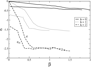
Figure 1: Comparison of the energy $e$ of a small-world system in which spin configurations can visit all possible configurations against the energy $e_{m}$ of the metastable configurations, plotted as function of the inverse temperature $\beta$ and for $J_{0}=\{0,1,2\}$. We see that $e_{m}<e$ and that for $\beta\to\infty$ $e_{m}\approx e$. Parameter values: $J=1$, $p=1$ and $c=2$.

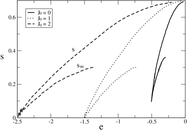
Figure 2: Comparison of the entropy $s$ of a small-world system in which spin configurations can visit all possible configurations against the entropy $s_{m}$ of the metastable configurations, plotted against their energy $e,e_{m}$, for $J_{0}=\{0,1,2\}$. For $J_{0}=0$ the ground state entropy has a finite value which vanishes as soon as $J_{0}>0$. Parameters values: $J=1$, $p=1$ and $c=2$.

In figure 2 we plot the entropy against the energy for different values of $J_{0}$, and with $p=1$, $J=1$, $c=2$. The low-energy part of the graph corresponds to regimes of low temperatures. As before, we compare the entropy $s$ that would follow from a thermodynamic calculation in the entire configuration space against the entropy $s_{m}$ of the metastable states. First, we see that one always has $s_{m}\leq s$, as one would expect. The difference between the two entropies varies significantly across the energy axis. For instance, for high energy values (where the temperature is practically infinite) this difference reaches its maximum value. On the other hand, for low temperatures, both entropies reach their minimum value which for any $J_{0}>0$ is zero. In the special case where $J_{0}=0$ the graph will typically consist of disconnected clusters which causes the observed degeneracy. However, as soon as the ‘ring’ connects all spins together this degeneracy is lost and the ground state entropy is zero.

Let us now examine the case of bond-disorder. In figure 3 we present the entropies $s$ and $s_{m}$ against the energy for different values of $J_{0}$ and with $J=1$, $c=2$, $p=1/2$. Firstly, we observe that the ground state energy is significantly higher compared to the case of $p=1$. This is due to the value of the local fields which will on average be smaller for $p<1$ than for $p=1$. We also observe that the ground state entropy can take a non-zero finite value even at $J_{0}>0$. This is due to the presence of anti-ferromagnetic couplings in the system which increases the fraction of sites with a zero local field. However, as one increases the strength of the (ferromagnetic) short-range couplings this fraction of sites becomes smaller and the degeneracy of the ground state gradually disappears. To illustrate this effect we plot in figure 4 the ground state entropy against the short-range coupling strength $J_{0}$. We also see a ‘jump’ precisely at $J_{0}=0$.

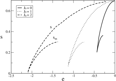
Figure 3: We show the entropies $s$ and $s_{m}$ for small-worlds with bond-disorder. In this case the degeneracy of the ground state remains finite even for $J_{0}>0$. Parameter values: $J=1$, $p=1/2$ and $c=2$.

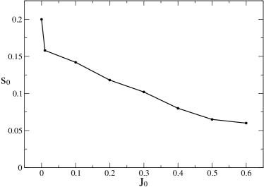
Figure 4: The ground state entropy density $s_{0}$ for a small-world system with bond-disorder as a function of $J_{0}$. There is a distinct jump precisely at $J_{0}=0$ while the entropy remains finite even for $J_{0}>0$. Parameter values: are $J=1$, $p=1/2$ and $c=2$.

VI Discussion

In recent years, the theory of complex networks has witnessed a remarkable growth. Within the area of complex systems, the special subset of ‘small-worlds’, has aroused the curiosity of theorists and experimentalists alike due to the striking cooperativity phenomena that they allow. In particular, for any value of the average long-range connectivity (however small), small-world networks can have a phase transition to an ordered phase at a finite temperature. Small world architectures have been observed in a wide range of real complex systems.

For a theorist, several important questions arise regarding the emergent collective properties on such systems. In this paper we have evaluated the number of metastable configurations. In a spirit similar to gardner ; bergsellito ; pagnani the ‘metastability’ condition constrains the partition sum over configurations in which spins align to their local fields. From an analytic point of view, two are the main stumbling blocks: firstly, the non-linear nature of the stability condition, and secondly, the diagonalisation of the relevant transfer matrix. Our numerical results suggest that, for low temperatures and in the case of bond-disorder, the metastable configurations tend to dominate the space of equilibrium states. We also see that superimposing the one-dimensional ‘backbone’ structure leads to a significantly smaller degeneracy of the ground state (which, in fact, vanishes for strictly ferromagnetic couplings). As function of the short-range coupling $J_{0}$, there is a jump in the ground state entropy exactly at $J_{0}=0$ which is due to the formation of disconnected clusters within the graph.

Appendix A Derivation of the saddle-point expression (9)

Our starting point are equations (6-8). We replace the delta function in (8) by its integral representation which results in

$$\left\langle Z^{n}\right\rangle_{\mbox{\boldmath$c$},\mbox{\boldmath$J$}}\equiv\left\langle\sum_{\mbox{\boldmath$\sigma$}^{1}\cdots\mbox{\boldmath$\sigma$}^{n}}e^{-\beta\sum_{\alpha}\mathcal{H}(\mbox{\boldmath$\sigma$}^{\alpha})}\prod_{i,\alpha}\Theta(\sigma_{i}^{\alpha}h_{i}(\mbox{\boldmath$\sigma$}^{\alpha}))\right\rangle_{\mbox{\boldmath$c$},\mbox{\boldmath$J$}}$$

$$=\int[\prod_{\mbox{\boldmath$\sigma$},\mbox{\boldmath$\tau$},\mathcal{J}}dP_{\mathcal{J}}(\mbox{\boldmath$\sigma$},\mbox{\boldmath$\tau$})d\hat{P}_{\mathcal{J}}(\mbox{\boldmath$\sigma$},\mbox{\boldmath$\tau$})]\exp\left[i\sum_{\mbox{\boldmath$\sigma$},\mbox{\boldmath$\tau$}}\sum_{\mathcal{J}}\hat{P}_{\mathcal{J}}(\mbox{\boldmath$\sigma$},\mbox{\boldmath$\tau$})P_{\mathcal{J}}(\mbox{\boldmath$\sigma$},\mbox{\boldmath$\tau$})+\frac{cN}{2}\left(\sum_{\mbox{\boldmath$\sigma$}\mbox{\boldmath$\tau$}}\left\langle P_{\mathcal{J}}(\mbox{\boldmath$\sigma$},\mbox{\boldmath$\tau$})P_{\mathcal{J}}(\mbox{\boldmath$\tau$},\mbox{\boldmath$\sigma$})\right\rangle_{\mathcal{J}}\right)\right]$$

$$\times\ \sum_{\mbox{\boldmath$\sigma$}^{1}\cdots\mbox{\boldmath$\sigma$}^{n}}\int\{dh_{i}^{\alpha}\}\prod_{\alpha}e^{\frac{1}{2}\beta\sigma_{i}^{\alpha}h_{i}^{\alpha}}\Theta(\sigma_{i}^{\alpha}h_{i}^{\alpha})$$

$$\times\ \prod_{i=1}^{N}\left\{\int\frac{\{d\hat{h}_{i}^{\alpha}\}}{(2\pi)^{n}}e^{i\sum_{i,\alpha}\hat{h}_{i}^{\alpha}(h_{i}^{\alpha}-J_{0}(\sigma_{i+1}^{\alpha}+\sigma_{i-1}^{\alpha}))}\sum_{\mu\geq 0}\frac{1}{\mu!}\sum_{\mbox{\boldmath$\tau$}_{1}\cdots\mbox{\boldmath$\tau$}_{\mu}}\sum_{\mathcal{J}_{1}\cdots\mathcal{J}_{\mu}}\left(\prod_{\nu\leq\mu}-i\hat{P}_{\mathcal{J}_{\nu}}(\mbox{\boldmath$\sigma$}_{i},\mbox{\boldmath$\tau$}_{\nu})\,e^{-i\frac{\mathcal{J}_{\nu}}{c}\sum_{\alpha}\hat{h}_{i}^{\alpha}\tau_{\nu}^{\alpha}}\right)\right\}.$$

We now see that the last line of the above expression has factorised over site indices and the integral over the variables $\{\hat{h}_{i}^{\alpha}\}$ can be done immediately. The result is a delta function which we use to eliminate $\{h_{i}^{\alpha}\}$:

$$\left\langle Z^{n}\right\rangle_{\mbox{\boldmath$c$},\mbox{\boldmath$J$}} = \int[\prod_{\mbox{\boldmath$\sigma$},\mbox{\boldmath$\tau$},\mathcal{J}}dP_{\mathcal{J}}(\mbox{\boldmath$\sigma$},\mbox{\boldmath$\tau$})d\hat{P}_{\mathcal{J}}(\mbox{\boldmath$\sigma$},\mbox{\boldmath$\tau$})]\exp\left[i\sum_{\mbox{\boldmath$\sigma$},\mbox{\boldmath$\tau$}}\sum_{\mathcal{J}}\hat{P}_{\mathcal{J}}(\mbox{\boldmath$\sigma$},\mbox{\boldmath$\tau$})P_{\mathcal{J}}(\mbox{\boldmath$\sigma$},\mbox{\boldmath$\tau$})+\frac{cN}{2}\left(\sum_{\mbox{\boldmath$\sigma$}\mbox{\boldmath$\tau$}}\left\langle P_{\mathcal{J}}(\mbox{\boldmath$\sigma$},\mbox{\boldmath$\tau$})P_{\mathcal{J}}(\mbox{\boldmath$\tau$},\mbox{\boldmath$\sigma$})\right\rangle_{\mathcal{J}}\right)\right]$$ (30)

$$\times\ \sum_{\mbox{\boldmath$\sigma$}^{1}\cdots\mbox{\boldmath$\sigma$}^{n}}\prod_{i=1}^{N}\left\{\sum_{\mu\geq 0}\frac{(-i)^{\mu}}{\mu!}\sum_{\mbox{\boldmath$\tau$}_{1}\cdots\mbox{\boldmath$\tau$}_{\mu}}\sum_{\mathcal{J}_{1}\cdots\mathcal{J}_{\mu}}\prod_{\nu\leq\mu}[\hat{P}_{\mathcal{J}_{\nu}}(\mbox{\boldmath$\sigma$}_{i},\mbox{\boldmath$\tau$}_{\nu})]\right.$$

$$\times\left.\int\{dh_{i}^{\alpha}\}\prod_{\alpha}e^{\frac{1}{2}\beta\sigma_{i}^{\alpha}h_{i}^{\alpha}}\Theta(\sigma_{i}^{\alpha}h_{i}^{\alpha})\ \delta\left[h_{i}^{\alpha}-J_{0}(\sigma_{i+1}^{\alpha}+\sigma_{i-1}^{\alpha})-\frac{1}{c}\sum_{\nu=1}\mathcal{J}_{\nu}\tau_{\nu}^{\alpha}\right]\right\}$$

$$= \int[\prod_{\mbox{\boldmath$\sigma$},\mbox{\boldmath$\tau$},\mathcal{J}}dP_{\mathcal{J}}(\mbox{\boldmath$\sigma$},\mbox{\boldmath$\tau$})d\hat{P}_{\mathcal{J}}(\mbox{\boldmath$\sigma$},\mbox{\boldmath$\tau$})]\exp\left[i\sum_{\mbox{\boldmath$\sigma$},\mbox{\boldmath$\tau$}}\sum_{\mathcal{J}}\hat{P}_{\mathcal{J}}(\mbox{\boldmath$\sigma$},\mbox{\boldmath$\tau$})P_{\mathcal{J}}(\mbox{\boldmath$\sigma$},\mbox{\boldmath$\tau$})+\frac{cN}{2}\left(\sum_{\mbox{\boldmath$\sigma$}\mbox{\boldmath$\tau$}}\left\langle P_{\mathcal{J}}(\mbox{\boldmath$\sigma$},\mbox{\boldmath$\tau$})P_{\mathcal{J}}(\mbox{\boldmath$\tau$},\mbox{\boldmath$\sigma$})\right\rangle_{\mathcal{J}}\right)\right]$$

$$\times\ \sum_{\mbox{\boldmath$\sigma$}^{1}\cdots\mbox{\boldmath$\sigma$}^{n}}\prod_{i=1}^{N}\left\{\sum_{\mu\geq 0}\frac{(-i)^{\mu}}{\mu!}\sum_{\mbox{\boldmath$\tau$}_{1}\cdots\mbox{\boldmath$\tau$}_{\mu}}\sum_{\mathcal{J}_{1}\cdots\mathcal{J}_{\mu}}\prod_{\nu\leq\mu}[\hat{P}_{\mathcal{J}_{\nu}}(\mbox{\boldmath$\sigma$}_{i},\mbox{\boldmath$\tau$}_{\nu})]\right.$$

$$\times\ \left.\prod_{\alpha}e^{\frac{1}{2}\beta\sigma_{i}^{\alpha}(J_{0}(\sigma_{i+1}^{\alpha}+\sigma_{i-1}^{\alpha})-\frac{1}{c}\sum_{\nu=1}\mathcal{J}_{\nu}\tau_{\nu}^{\alpha})}\ \Theta\left(\sigma_{i}^{\alpha}(J_{0}(\sigma_{i+1}^{\alpha}+\sigma_{i-1}^{\alpha})+\frac{1}{c}\sum_{\nu=1}\mathcal{J}_{\nu}\tau_{\nu}^{\alpha})\right)\right\}$$

With the above, the generating function (4) can be written as an extremisation problem, namely:

$$-\beta f=\lim_{n\to 0}\frac{1}{n}\underset{P,\hat{P}}{\rm Extr}\left[i\sum_{\mbox{\boldmath$\sigma$},\mbox{\boldmath$\tau$}}\sum_{\mathcal{J}}\hat{P}_{\mathcal{J}}(\mbox{\boldmath$\sigma$},\mbox{\boldmath$\tau$})P_{\mathcal{J}}(\mbox{\boldmath$\sigma$},\mbox{\boldmath$\tau$})+\frac{c}{2}\sum_{\mbox{\boldmath$\sigma$}\mbox{\boldmath$\tau$}}\left\langle P_{\mathcal{J}}(\mbox{\boldmath$\sigma$},\mbox{\boldmath$\tau$})P_{\mathcal{J}}(\mbox{\boldmath$\tau$},\mbox{\boldmath$\sigma$})\right\rangle_{\mathcal{J}}+\lim_{N\to\infty}\frac{1}{N}\log\,{\rm tr}\,(\tilde{T}^{N}[\hat{P}])\right]$$ (31)

with the transfer function $\tilde{T}[\hat{P}]$ given by

$$\tilde{T}_{\mbox{\boldmath$\sigma$}_{i-1},\mbox{\boldmath$\sigma$}_{i},\mbox{\boldmath$\sigma$}_{i+1}}[\hat{P}] = \sum_{\mu\geq 0}\frac{(-i)^{\mu}}{\mu!}\sum_{\mbox{\boldmath$\tau$}_{1}\cdots\mbox{\boldmath$\tau$}_{\mu}}\sum_{\mathcal{J}_{1}\cdots\mathcal{J}_{\mu}}\prod_{\nu\leq\mu}[\hat{P}_{\mathcal{J}_{\nu}}(\mbox{\boldmath$\sigma$}_{i},\mbox{\boldmath$\tau$}_{\nu})]$$ (32)

$$\times\ \prod_{\alpha}e^{\frac{1}{2}\beta\sigma_{i}^{\alpha}(J_{0}(\sigma_{i+1}^{\alpha}+\sigma_{i-1}^{\alpha})-\frac{1}{c}\sum_{\nu=1}\mathcal{J}_{\nu}\tau_{\nu}^{\alpha})}\ \Theta\left(\sigma_{i}^{\alpha}(J_{0}(\sigma_{i+1}^{\alpha}+\sigma_{i-1}^{\alpha})+\frac{1}{c}\sum_{\nu=1}\mathcal{J}_{\nu}\tau_{\nu}^{\alpha})\right)$$

Variation of (31) with respect to the function $P_{\mathcal{J}}$ gives the relation $\hat{P}_{\mathcal{J}}(\mbox{\boldmath$\sigma$},\mbox{\boldmath$\tau$})=icQ_{J}(\mathcal{J})\,P_{\mathcal{J}}(\mbox{\boldmath$\tau$},\mbox{\boldmath$\sigma$})$ for $\mathcal{J}=\{-J,J\}$. Using this identity in (31) leads to (9).

References

• (1) Milgram S (1967) Psychology Today 2 60
• (2) Watts D J and Strogatz S H (1998) Nature 393 440
• (3) Girvan M and Newman M E J (2002) PNAS 99 7821
• (4) Siming L et al (2004) Science 303 540-543
• (5) Barabási A-L and Oltvai Z N (2004) Nature Rev Gen 5 101
• (6) Newman M E J (2001) PNAS 98 404
• (7) Barrat A and Weigt M (2000) Eur Phys J B 13 547
• (8) Nikoletopoulos T, Coolen A C C, Pérez Castillo I, Skantzos N S, Hatchett J P L and Wemmenhove B (2004) J Phys A 37 6455
• (9) Albert R and A-L Barabási (2002) Rev Mod Phys 74 47
• (10) Newman M E J (2003) SIAM review 45 167
• (11) Duncan J Watts (2003) ‘Small Worlds: The Dynamics of Networks between Order and Randomness’, Princeton University Press.
• (12) S.N. Dorogovtsev and J.F.F. Mendes (2003) ‘Evolution of Networks: From Biological Nets to the Internet and WWW’, Oxford University Press.
• (13) Skantzos N S, Pérez Castillo I and Hatchett J P L (2005) submitted to Phys Rev E cond-mat:0508609
• (14) Nikoletopoulos T and Coolen A C C (2004) J Phys A 37 8433
• (15) Berg J and Sellito M (2002) Phys Rev E 65 016115
• (16) A Pagnani, G Parisi and M Ratiéville (2003) Phys Rev E 67 026116
• (17) Lefevre A and Dean DS (2001) Eur Phys J B 21 121
• (18) Mézard M and Parisi G (2001) Eur Phys J B 20 217
• (19) Mézard M and Parisi G (2003) J Stat Phys 111 1
• (20) Leone M, Vazquez A, Vespignani A and Zecchina R (2002) Eur Phys J B 28 191
• (21) Boettcher S (2003) Phys Rev B 67 060403
• (22) Boettcher S (2003) Eur Phys Jour B 31 29
• (23) Gardner E (1986) J Phys A 19 L1047
• (24) Bray A J and Moore M A (1981) J Phys C 14 1313
• (25) Wemmenhove B, Nikoletopoulos T, Hatchett J P L (2004) condmat:0405563, to appear in J Stat Phys
• (26) Pérez Castillo I, Wemmenhove B, Hatchett JPL, Coolen ACC, Skantzos NS, Nikoletopoulos T (2004) J Phys A 37 8789