A model of a dual-core matter-wave soliton laser

Abstract

We propose a system which can generate a periodic array of solitary-wave pulses from a finite reservoir of coherent Bose-Einstein condensate (BEC). The system is built as a set of two parallel quasi-one-dimensional traps (the reservoir proper and a pulse-generating cavity), which are linearly coupled by the tunneling of atoms. The scattering length is tuned to be negative and small in the absolute value in the cavity, and still smaller but positive in the reservoir. Additionally, a parabolic potential profile is created around the center of the cavity. Both edges of the reservoir and one edge of the cavity are impenetrable. Solitons are released through the other cavity’s edge, which is semi-transparent. Two different regimes of the intrinsic operation of the laser are identified: circulations of a narrow wave-function pulse in the cavity, and oscillations of a broad standing pulse. The latter regime is stable, readily providing for the generation of an array containing up to $10,000$ permanent-shape pulses. The circulation regime provides for no more than $40$ cycles, and then it transforms into the oscillation mode. The dependence of the dynamical regime on parameters of the system is investigated in detail.

I Introduction

The concept of matter-wave lasers, which are intended to generate strong coherent beams of atoms, and many applications that such beams can find, are well known. It is commonly assumed that a Bose-Einstein condensate (BEC) may serve as a source of the matter-wave laser beam. Atomic lasing was considered in detail theoretically (see Refs. laser and references therein) and demonstrated in various experimental settings experiment ; the topic was recently reviewed in Ref. review . Of special interest is a possibility to construct a laser operating in a pulsed (quasi-soliton) regime, i.e., periodically releasing narrow localized pulses of coherent atom waves, as proposed in Refs. soliton-laser and Carr . In that connection, it is relevant to mention that (effectively) one-dimensional solitons in BEC with very weak attraction between atoms (in ⁷Li) were created in well-known experiments soliton .

The first models of the pulsed matter-wave lasers assumed release of quasi-solitons from an elongated (“cigar-shaped”) trap filled by a self-attractive BEC. This scheme, while probably realizable in the experiment, does not offer sufficiently effective means to control the operation regime, and does not secure generation of a very large number of pulses in a nearly periodic fashion. A more sophisticated scheme was very recently proposed in Ref. Spain , which assumes zero nonlinearity coefficient (i.e., zero scattering length of inter-atomic collisions) in a larger part of the elongated trap, and attraction between atoms (negative scattering length) in its smaller part, where the pulses are to be formed and released. The sign of the scattering length may be controlled and altered along the length of the trap by means of the Feshbach resonance Feshbach (this mechanism was used for the experimental creation of the BEC solitons soliton ).

In this work, we aim to propose a different model of a pulsed matter-wave laser, in which the BEC reservoir and the pulse-generating cavity are separated. As shown in Fig. 1 below, they are elongated parallel traps with linear coupling between them, due to tunneling of atoms. Using the aforementioned possibility to control the scattering length by means of the Feshbach resonance, we assume that the interaction between atoms is (very weakly) repulsive in the reservoir, while in the cavity it is attractive (and weak too, see below). Additionally, the negative scattering length is assumed to be altered along the cavity’s axis, which can be achieved using an appropriate configuration of the magnetic field responsible for the Feshbach resonance (we do not assume any time dependence of the scattering length or other parameters).

Besides using the magnetic field, it was predicted theoretically optFRtheory and demonstrated experimentally optFRexperiment that the Feshbach resonance can be provided too by an adequately tuned optical field. Accordingly, a spatially modulated stationary distribution of the light intensity may also be employed to provide for necessary spatially inhomogeneous Feshbach-resonance configurations in the reservoir and cavity.

It is relevant to mention that various soliton solutions in dual-core traps, with the linear coupling between the cores and opposite signs of the scattering length in them, were recently studied in detail Valery , following an earlier work which was dealing with a model of dual-core nonlinear optical fibers with opposite signs of the group-velocity dispersion (rather than nonlinearity) in the two cores Dave .

In the model introduced below, both edges of the reservoir, and the left edge of the cavity are impenetrable to atoms, while the right edge of the cavity (a “valve”) allows the release of pulses into an outcoupling atomic waveguide, see Fig. 1. The model was originally designed with an intention to provide for formation of a narrow quasi-soliton pulse in the cavity, that would periodically circulate in it, bouncing from the edges. Each time that the soliton hits the right edge (valve), a pulse is released into the outcoupling waveguide. After being slashed this way, the intrinsic solitary pulse is supposed to replenish itself in the course of the subsequent cycle of the circulation by collecting atoms tunneling from the reservoir. Accordingly, the initial condition is taken with a large number of atoms in the reservoir, and a small number in the cavity.

As described in detail below, numerical simulations demonstrate that the circulation regime outlined above may be observed, but it is not a really stable one: the intrinsic pulse would perform no more than $40$ circulations, quickly coming to a halt and getting broad. Nevertheless, a very robust regime of the periodic release of pulses can be found in a large parameter region. In this regime, a broad “lump” stays immobile in the cavity, performing periodic cycles of stretching and compression. When its right wing reaches the valve, in the course of each cycle of the vibrations, a new outcoupling pulse is released. The respective loss in the number of atoms in the cavity is compensated by the influx of atoms tunneling from the reservoir. The pulse-release cycles repeat very many times, till the reservoir gets essentially depleted. We stress that the model is a passive one, i.e., it supports the stable pulse generation regime without any externally applied active control, such as periodically opening and shutting the valve by some clock signal.

Figure 1: A scheme of the proposed matter-wave laser composed of two nearly one-dimensional traps coupled by tunneling of atoms, with negative and positive scattering lengths in the cavity and reservoir, respectively. The opening at the right edge of the cavity ($x=1$) depicts the valve releasing pulses into an outcoupling waveguide. Shading symbolically shows an instantaneous density distribution, $\left|\psi\right|^{2}$ and $\left|\phi\right|^{2}$, in both traps (larger density corresponds to more intense shading). The upper part shows the potential profile in the cavity, with the drop $\Delta U$ at $x=1$ corresponding to the valve.

The paper is organized as follows. In Section 2, the model is formulated. Basic results, which demonstrate both unstable circulation-based and stable vibration-based regimes of the periodic generation of solitary pulses, are presented in Section 3. In Section 4, we analyze the dependence of the operation of the matter-wave laser on its parameters, and give an estimate for the actual number of atoms in outcoupled pulses generated by the laser. The paper is concluded by Section 4.

II The model

According to what was said above, the model of the matter-wave laser is based on a system of linearly coupled Gross-Pitaevskii equations (GPEs) for the wave functions $\psi(x,t)$ and $\phi(x,t)$ of atoms in the (effectively) one-dimensional cavity and reservoir, with opposite signs in front of the nonlinear terms. We scale $\hbar$, the atomic mass $m$, and the nonlinearity coefficient at $x=0$ in the cavity (in physical units, the latter is $4\pi\hbar^{2}a/m$, where $a$ is the $s$-wave scattering length of atomic collisions around $x=0$) to be $1$. Then, the coupled equations are cast in a normalized form,

$$i\psi_{t} = -\frac{1}{2}\psi_{xx}-\left(1+gx\right)|\psi|^{2}\psi$$ (1)

$$+f(x-L/2)^{2}\psi-\kappa\phi,$$

$$i\phi_{t} = -\frac{1}{2}\phi_{xx}+\epsilon|\phi|^{2}\phi-\kappa\psi,$$ (2)

where the coordinate $x$ takes values $0<x<L$ (i.e., $L$ is the length of both the cavity and reservoir). In accordance with what was said above, we assume a small positive scattering length (weak repulsion between atoms) in the reservoir, $\epsilon>0$, while in the cavity the interaction is attractive, with the strength linearly increasing with $x$ ($g>0$ is assumed), following a corresponding profile of the static magnetic or optical field that controls the scattering length in the cavity via the Feshbach resonance.

The coefficient $g$ will be small (see below), but it is needed to create an effective potential slope in the cavity: as the intra-cavity pulse gets “heavier” due to the agglomeration of atoms tunneling from the reservoir, the term proportional to $g$ creates a gradually increasing effective potential which pushes atoms to the right (since $g$ is positive). In the aforementioned circulation regime, this effective (nonlinear) potential pushes the intra-cavity localized pulse to the right. After hitting the right edge (at $x=L$), where the “valve” is placed (see details below), the pulse loses a part of its mass, generating the outcoupled soliton. Therefore, the force induced by the nonlinear potential drops, allowing the intra-cavity pulse to move in the opposite direction after the bounce from the right edge, until it will bounce (without loss) from the left edge, $x=0$. This way, the nonlinear term proportional to $g$ may support periodic circulations of the internal pulse (although, as said above, in the domain of the model’s parameter space explored in this work the circulations are not really stable, eventually switching into the regime of vibrations; the latter regime is possible with $g=0$ as well).

Further, we assume that an external parabolic potential acts in the cavity,

$$U_{\mathrm{pot}}(x)=f(x-L/2)^{2},$$ (3)

with the center set at the middle of the cavity. It is well known that such a potential corresponds to a magnetic or optical trap applied to the condensate optical . It will be shown below that the results are not sensitive to the exact shape of the intra-cavity potential; in fact, essentially the same stable vibration regime can be obtained in the model with no potential.  Note that Eq. (2) for the reservoir does not include any potential, as it is not necessary to generate the dynamical regime sought for. We also explored a model including a potential in the reservoir, but it did not affect the operation regime in any remarkable manner.

The linear coupling between the cavity and reservoir is accounted for by the positive coefficient $\kappa$, which determines the tunneling time $1/\kappa$ for atoms. Keeping $\epsilon,g,f$ and $\kappa$ as free parameters of the model, the remaining scaling invariance of Eqs. (1) and (2) makes it possible to set $L\equiv 1$, which is fixed below.

As said above, the model assumes that the reservoir at its both edges, and the cavity at its left edge are closed by impenetrable lids, which gives rise to the respective boundary conditions (b.c.),

$$\phi(x=0)=\phi(x=1)=\psi(x=0)=0.$$ (4)

The pulses (solitons) are to be released into an external waveguide from the cavity at its right edge, $x=1$ (recall we have set $L\equiv 1$). For this purpose, a valve is set at $x=1$, assuming that the corresponding b.c. for the $\psi$ field is linear. Actually, the single possible form of such a linear b.c. is

$$\psi_{x}(x=1)=iq\psi(x=1),$$ (5)

with a positive constant $q$ (its physical meaning is discussed below). Indeed, using the continuity equation for the total density, $\rho\equiv|\psi|^{2}+|\phi|^{2}$, and current, $j=(i/2)\left(\psi_{x}^{\ast}\psi-\psi_{x}\psi^{\ast}\right)+(i/2)\left(\phi_{x}^{\ast}\phi-\phi_{x}\phi^{\ast}\right)\equiv j_{1}+j_{2}$, in the coupled GPEs (1) and (2),

$$\frac{\partial\rho}{\partial t}=\frac{i}{2}\left(\psi_{xx}\psi^{\ast}-\psi_{xx}^{\ast}\psi\right)\equiv-\frac{\partial j}{\partial x},$$ (6)

integrating Eq. (6) over the length of the system, $0<x<1$, and taking into regard that $j_{1}(x=0)=j_{2}(x=0)=j_{2}(x=1)=0$ pursuant to b.c. (4), one can derive a depletion equation for the solution’s norm $N$, which is proportional to the total number of atoms in the system:

$$N = \int_{0}^{1}\left(|\psi(x)|^{2}+|\phi(x)|^{2}\right)dx\equiv N_{1}+N_{2},$$ (7)

$$-\frac{dN}{dt} = j_{1}(x=1,t)=q\left|\psi(x=1,t)\right|^{2}\equiv E(t),$$ (8)

where b.c. (5) was substituted for $\psi_{x}$ in the expression for $j_{1}(x=1)$. The latter result is what might be expected: the instantaneous rate at which the density is released through the valve is proportional to the local density $\left|\psi(x=1)\right|^{2}$, which justifies the adoption of b.c. (5). Initial values of the norms $N_{1}^{(0)}$ and $N_{2}^{(0)}$ of the $\psi$ and $\phi$ fields, and the b.c. constant $q$ are supplementary control parameters of the model, in addition to the above-mentioned set of $\left(\epsilon,g,f,\kappa\right)$. Below, it will be demonstrated that really important parameters are $\epsilon$, $\kappa$, and $q$.

The physical meaning of b.c. (5) can be readily understood. Indeed, it implies that the local gradient of the phase of the wave function $\psi$ at the point $x=1$, which is proportional to the atom’s momentum, is fixed to be $q$. This can be realized by assuming that, to the right of the point $x=0$ (in the outcoupling waveguide), the cavity potential drops by $\Delta U=q^{2}/2$ (recall we have set $m=\hbar=1$). The drop $\Delta U$ must be essentially larger than the potential and kinetic energy of atoms to the left of the point $x=1$ (in the cavity). The latter condition, which amounts to

$$U(x=1)=f/4\ll q^{2}/2$$ (9)

[see Eq. (3)], provides for the possibility to neglect small deviations in the kinetic energy of the released atoms from $q^{2}/2$. We notice that a soliton-releasing valve in the matter-wave laser model recently proposed in Ref. Spain includes a similar element (an effective potential step).

The form of the function $E(t)$, as defined in Eq. (8), determines the shape of the density pattern (actually, an array of pulses) released into the outcoupling waveguide, the same way as the temporal shape of the input signal at the point $z=0$ determines the shape of a temporal soliton or solitonic array propagating along the coordinate $z$ in the optical fiber Agrawal . Note that, as follows from Eq. (5), the limit cases of $q=0$ and $q=\infty$ correspond, respectively, to a reflecting mirror and impenetrable lid, i.e., $\psi_{x}(x=1)=0$ and $\psi(x=1)=0$. In either case, the system does not release anything. In addition to yielding the final result in the form of $E(t)$, Eq. (8), with $dN/dt$ computed directly from numerical data, provides for a means to monitor the accuracy of simulations.

Finally, we note that the model does not include an explicit form of the outcoupling waveguide (the extension of the cavity beyond $x=1$), which is responsible for the eventual shaping the released pulses into solitons. Actually, the soliton-formation problem in a uniform waveguide has been studied in detail before (see, e.g., Ref. Carr and references therein).

III Operation regimes of the pulsed matter-wave laser

In the numerical analysis of the model, Eqs. (1) and (2) were solved by means of a finite-element pseudospectral method, which implies division of the integration domain into several finite elements. Solution in each element is approximated by a polynomial, and a pseudo-spectral method, based on Chebyshev collocation points Peter , is used in each element. We have checked that a numerical algorithm based on domain stretching, rather than domain division into finite elements Chebyshev , produces the same results.

In cases when the stationary version of the GPEs, i.e., a system of two linearly coupled ordinary differential equations, had to be solved (see below), the finite-element pseudospectral method reduces them to a set of algebraic equations, which were treated by means of the Newton’s method. In the general case, when Eqs. (1) and (2) are partial differential equations, the time derivatives in the equations were approximated by the finite difference as per the Crank-Nicholson scheme. This, together with the finite-element pseudospectral method, yields a set of nonlinear algebraic equations, that were also solved by the Newton’s algorithm.

In all the cases considered, the integration domain $0\leq x\leq 1$ was divided into four equal elements, with a fifth-order polynomial used in each one. The procedure leads to a set of $48$ algebraic equations, and it was checked that increase of the polynomial’s order did not change the results in any tangible aspect. We used the time step of $\Delta t=0.001$, checking that smaller time steps gave virtually the same results (while larger $\Delta t$ would generally be insufficient to produce accurate results).

Simulations started with initial conditions which, by themselves, were stationary solutions to Eqs. (1) and (2), in the form of $\left\{\psi(x,t),\phi(x,t)\right\}=\exp\left(-i\mu t\right)\left\{\Psi(x),\Phi(x)\right\}$ with real $\Psi(x)$ and $\Phi(x)$. These stationary solutions were found, in a numerical form, for given values of $g,\epsilon$ and $\kappa$. While doing so, b.c. (5) at $x=1$ was temporarily replaced by $\psi=0$ [as said above, this formally corresponds to $q=\infty$ in Eq. (5)], since a stationary solution is not possible otherwise, due to the nonzero current $j_{1}$ across the point $x=1$, see Eq. (6). Further, both equations (1) and (2) used to generate the stationary solutions were modified by including ad hoc potentials linear in $x$, as the so generated initial configurations were found to quickly produce stable operation regimes, even though the actual potentials in Eqs. (1) and (2) are different [recall that Eq. (2) has no potential at all]. A set of typical initial configurations obtained this way is displayed in Fig. 2.

$\begin{array}[]{cc}\includegraphics[width=267.39877pt]{fig1a.eps}&\includegraphics[width=267.39877pt]{fig1b.eps}\end{array}$

Figure 2: Typical examples of the initial real profiles of $\Psi(x)$ (a) and $\Phi(x)$ (b) for $g_{1}=0.02$, $\epsilon=0.1$, and $\kappa=0.5$, used in simulations of the coupled equations (1) and (2). In all the cases, the norm of the $\phi$-component is fixed (in the normalized units) to be $N_{2}=363.4$, while the norm $N_{1}$ of the $\psi$-component varies as shown in the figure.

Starting from such initial configurations, simulations produced two types of dynamical regimes. The first one features a relatively narrow pulse which performs shuttle motion, circulating in the cavity. Each collision of the pulse with the valve at the right edge of the cavity gives rise to a quasi-soliton released by the matter-wave laser. However, as mentioned above, the circulation regime was never found to be stable (although we cannot claim that the investigation of the system’s parameter space was exhaustive, as it is difficult to perform complete exploration of the seven-paramater space). The pulse would perform no more than $40$ circulations (typically, fewer), and this regime would transform itself into a stable vibration regime.

An example of the transition from circulations to vibrations is displayed in Fig. 3. Actually, the transition may be much shorter at other values of the parameters. In most cases, as shown below, the vibration regime sets in directly from the initial configuration, without going through the transient stage of circulations.

$\begin{array}[]{cc}\includegraphics[width=267.39877pt]{fig2b.eps}&\includegraphics[width=267.39877pt]{fig2c.eps}\end{array}$

Figure 3: Transition of the circulation regime into a vibration one, shown in terms of a three-dimensional plot for the density $|\psi(x,t)|^{2}$ in the cavity (a), contour plots of the density (b), and the outcoupling rate $E(t)$ (c). The parameters are $g=0.02$, $\epsilon=0.1$, $f=3$, $\kappa=0.5$, and $q=50$. The initial (normalized) numbers of atoms in the reservoir and cavity are $N_{2}^{(0)}=360$ and $N_{1}^{(0)}=12$.

The instability of the circulation regime can be understood. Indeed, one may consider a small fluctuation which makes the norm of the pulse released into the outcoupling waveguide slightly smaller than in the established regime, hence the norm remaining in the cavity soliton becomes slightly larger. Consequently, the strength of the effective nonlinear potential, that tries to push the soliton to the right, drops (as a results of the bounce from the valve) by an amount which is a bit smaller than in the unperturbed state, and the soliton will therefore slide to the left slower than in the absence of the perturbation. As a result, spending more time in the cavity, the soliton will absorb more atoms in the course of the next cycle of the circulations, and will return to the right edge with a still larger norm. The mechanism by which a fluctuation slightly increasing the soliton’s norm leads to its still larger increase (or, conversely, a fluctuation decreasing the norm causes its further decrease) implies the instability. It may happen that the circulation regime can be stabilized in a model including an active element (i.e., forced circulations might be stable), but in this work we focus on the more fundamental passive model.

In the regime of vibrations, a broad pulse stays at the center of the cavity and performs a very large number of internal oscillations. At a stage of the vibration cycle when the pulse spreads out, its right wing hits the valve and generates an outcoupling localized matter-wave packet. A typical example of such a stable regime is displayed in Figs. 4 and 5. The second panel in Fig. 4 shows (for a long interval of time) the temporal dependence of the outcoupling rate $E(t)$, as defined by Eq. (8). As said above, this dependence actually determines the shape of the pulse array released by the matter-wave laser.

$\begin{array}[]{cc}\includegraphics[width=267.39877pt]{fig3a.eps}&\includegraphics[width=267.39877pt]{fig3b.eps}\\ \includegraphics[width=267.39877pt]{fig3c.eps}&\includegraphics[width=267.39877pt]{fig3d.eps}\end{array}$

Figure 4: A typical example of the establishment of a stable vibration regime in the cavity, shown in terms of the outcoupling rate $E(t)$, which determines the shape of the pulse array generated by the matter-wave laser [$E$ is defined as per Eq. (8)]. (a) The initial stage; (b) beginning of the established regime; (c) a fragment from panel (b), showing 15 cycles in detail; (d) a single typical cycle (shown in terms of obviously rescaled variables $t^{\ast}$ and $E^{\ast}$), together with a simplest analytical fit to it. In panels (a) and (b), contour plots in the lower subpanels (ii) additionally illustrate the spatiotemporal evolution of the atom density, $\left|\psi(x,t)\right|^{2}$. Parameters are $g=0.02$, $\epsilon=0.10$, $f=3$, $\kappa=0.5$, and $q=200$. The initial normalized amounts of matter in the reservoir and cavity are $N_{2}=363.4$ and $N_{1}=6$. In the established regime, the period is $T=0.135$, with the duty cycle of $50\%$.

Figure 5: The evolution of the density distribution in the cavity, $|\psi(x,t)|^{2}$, for the same case as shown in Fig. 4.

Figure 5 depicts vibrations of the density distribution in the cavity, for the same case as displayed in Fig. 4. As seen from these figures, after a transient period, a very robust regime (with some residual long-period modulations) sets in. With the maximum value of the release rate $E$ in this regime $E_{\max}\simeq 0.4$, the oscillation period $T=0.135$ and the duty cycle (the share of the period within which the value of the density at the right edge of the cavity, $|\psi(x=1,t)|^{2}$, exceeds half of its maximum value) being $0.5$ imply that the number of cycles which are expected before depletion of the reservoir will become appreciable (say, $N$ will drop to two thirds of $N_{2}^{(0)}=363.4$) can be easily estimated:

$$\frac{(2/3)N_{2}^{(0)}}{E_{\max}\cdot(T/2)}\simeq 10,000\text{ {cycles}.}$$ (10)

Direct verification of this prediction requires too long simulations (up to $t\simeq 1500$). An estimate for the actual number of atoms in the generated pulses (which may range between $10$ and $1000$) is given in the next section.

It is relevant to stress that, in the cases presented in Figs. 3 and 4, 5, with $f=3$ and $q=200$, the condition (9), which substantiates the use of b.c. (5), is satisfied with a huge margin. In fact, this condition holds equally well in all the cases where stable operation of the matter-wave laser model was observed. It is also relevant to mention that, in physical units, the value of $q\sim 100$ corresponds, for ⁷Li, to the velocity $\sim 1$ cm/s of the released atoms, the respective kinetic energy being $\sim 0.1$ nK, on the temperature scale.

It is relevant to compare the depletion rate in the stable operation mode [as given by Eq. (8)] with the rate at which the cavity and reservoir exchange the matter. A generic example of this comparison is displayed in Fig. 6. As is seen, the exchange rate is much higher than the speed of depletion. It is interesting to note that the long-period beatings in the dependence of $N_{1}(t)$, which are observed in 6, practically do not manifest themselves in the oscillations of the outcoupling rate $E(t)$ [nor in the evolution of $N_{1}+N_{2}$, as the beatings in $N_{1}(t)$ are almost exactly compensated by anti-phase beatings in $N_{2}(t)$]. In other words, the beatings do not affect the quality of the pulse array generated by the matter-wave laser.

The line showing $N_{1}+N_{2}$ vs. $t$ in Fig. 6 seems to have finite thickness due to fast oscillations of $E(t)$, such as those in Fig. 4. Its comparison with the respective dependence predicted by averaging of the depletion equation (8) (a bold dashed line) is also shown in Fig. 6. An error due to the averaging may account for a small discrepancy with the actual evolution of $N_{1}+N_{2}$.

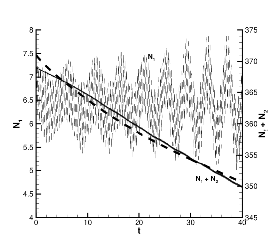
Figure 6: The evolution of the norm (amount of matter) in the reservoir, $N_{1}$ (the rapidly oscillating dashed curve), and the total norm, $N_{1}+N_{2}$ (the continuous finite-thickness line), in a stable operation regime. The bold dashed curve displays the prediction following from the depletion equation (8), averaged over rapid oscillations of $E(t)$. Parameters are the same as in Fig. 4.

IV Dependence of the operation regime on parameters

The matter-wave laser model proposed above depends on several parameters. It is necessary to identify those which are really important to the stability of the operation mode, and which are not. First of all, simulations demonstrate that there is virtually no dependence on the potential’s strength $f$ in Eq. (1): at least within the interval of $1<f<3$, all dynamical characteristics of the matter-wave laser model display very little variation, if other parameters are fixed (taking typical values of physical parameters given below, we conclude that, in this parameter region, the range of $1<f<3$ actually corresponds to the range of the longitudinal trapping frequencies $0.1-1$ Hz). The dependence on the initial amount of matter in the cavity, $N_{1}^{(0)}$, is very weak too, at least in the interval of $5<N_{1}^{(0)}<20$. Also negligible is sensitivity of the established regime to the parameter $g$ in Eq. (1). In fact, additional simulations have demonstrated that virtually the same stable oscillation regime sets in if we take Eqs. (1) and (2) with $f=g=0$.

A more important role is played by the constant $q$ in Eq. (5) (recall it determines the momentum of atoms in the outcoupling pulse), and the linear-tunneling constant $\kappa$ that determines the strength of the linear coupling between the reservoir and cavity in Eqs. (1) and (2). Figures 7 and 8 illustrate effects of the variation of these parameters on the operation regime. This is shown via the change of the time dependences of the outcoupling rate $E(t)$ and total amount of matter remaining in the system, $N_{1}+N_{2}$.

$\begin{array}[]{cc}\includegraphics[width=267.39877pt]{fig6a.eps}&\includegraphics[width=267.39877pt]{fig6b.eps}\end{array}$

Figure 7: The influence of the variation of the boundary-condition parameter $q$ (the momentum of atoms in pulses released by the matter-wave laser), see Eq. (5), on the time dependence of the outcoupling rate (a), and on the depletion dynamics (b). Except for $q$, other parameters are the same as in Fig. 4.

$\begin{array}[]{cc}\includegraphics[width=267.39877pt]{fig7a.eps}&\includegraphics[width=267.39877pt]{fig7b.eps}\end{array}$

Figure 8: The same as in Fig. 7, but showing the effect of the variation of the strength of the linear coupling between the reservoir and cavity.

The essential dependence of the dynamical regimes on the parameters $q$ and $\kappa$ is quite natural. In addition to this, and somewhat unexpectedly, the system demonstrates strong sensitivity to the value of the nonlinearity coefficient $\epsilon$ in Eq. (2), which is proportional to the positive atomic collision length in the reservoir. In fact, stable operation regimes, providing for the generation of very long periodic arrays of the outcoupling pulses, are possible in a relatively narrow interval of values of $\epsilon$, if the other parameters are fixed. The dependence of the dynamical states on $\epsilon$ is illustrated, by displaying segments of the established dependence $E(t)$, in Fig. 9. Panel (a) in this figure shows that, at $\epsilon=0.08$, the generated array of pulses has a high amplitude, but with shallow dips between pulses, so that they are not well separated. The same panel demonstrates that the optimum shape of the array of well-separated pulses is achieved between $\epsilon=0.09$ and $0.12$ (which implies the positive scattering length in the reservoir being $\simeq 10$ times smaller than the absolute value of the negative scattering length in the cavity). The situation in the latter interval is additionally illustrated by a set of curves in panel (b) of Fig. 9. Physically, the necessary fine-tuning of $\epsilon$ in the reservoir may be achieved by means of the Feshbach resonance.

$\begin{array}[]{cc}\includegraphics[width=267.39877pt]{fig8a.eps}&\includegraphics[width=267.39877pt]{fig8b.eps}\end{array}$

Figure 9: The effect of variation of the nonlinearity coefficient $\epsilon$ in the reservoir on the operation regime of the matter-wave laser model. Other parameters are the same as in Fig. 3.

Undoing normalizations that cast the coupled GPEs in the rescaled form of Eqs. (1) and (2), it is easy to derive a relation between the actual number of atoms, $N_{\mathrm{phys}}$, and the norm $N_{1}$ of the $\psi$ function in the normalized units:

$$N_{\mathrm{phys}}=\frac{r^{2}}{8|a|L}N_{1},$$ (11)

where $r$ is the transverse radius of the cigar-shaped trap, which plays the role of the cavity, $a$ and $L$ being, respectively (as defined above), the Feshbach resonance-controlled atomic scattering length in the cavity and the cavity’s length, both taken in physical units. For the cases displayed in Fig. 9, a characteristic value of the norm of an individual released pulse, in the normalized units, is $N_{1}\sim 0.1$. Assuming the aspect ratio of the cylindrical trap to be $L/(2r)\simeq 10$, and the actual length $L\simeq 100$ $\mu$m, Eq. (11) yields the number of atoms per outcoupling pulse between $10$ and $1000$, if the scattering length is kept at a low level, between $a\simeq-0.1$ nm and $a\simeq-0.01$ nm (a very small value of $|a|$ is necessary to prevent collapse in the cavity trap). These values may be sufficient for physical applications. In particular, the threshold number of ⁷Li atoms, necessary for the creation of a stable three-dimensional solitons in an optical lattice, was recently shown to be $60$ 3D . The number of atoms $\sim 100$ may also be sufficient for direct optical detection of the matter-wave pulse. As for the total number of atoms originally stockpiled in the reservoir, the above estimates, including Eq. (10), yield the range of $N_{0}\sim 10^{5}-10^{7}$ for it.

V Conclusion

The objective of this work was to propose a model of a matter-wave laser which can provide for stable periodic generation of a sequence of solitary-wave pulses from a reservoir containing a large amount of matter in the form of a coherent Bose-Einstein condensate. The system includes two parallel cigar-shaped traps, viz., the reservoir and the work cavity, which are coupled by the tunneling of atoms between them. The scattering length of atomic collisions is tuned to be positive and negative in the reservoir and cavity, respectively. Both ends of the reservoir, and the left edge of the cavity are closed by lids. Solitary pulses are released through a “valve” at the right edge of the cavity, which is described by the linear boundary condition (5), and may be implemented as a potential step separating the cavity and the outcoupling waveguide. Two different regimes of the operation of the matter-wave laser were identified: circulations of a narrow solitary pulse in the cavity, and vibrations of a broad standing lump. Only the latter mode is stable, while the circulation regime spontaneously rearranges itself into the vibration mode. Dependence of the stability and characteristics of the pulse-generating regime on parameters of the model was explored. The regime is sensitive to the boundary-condition parameter $q$ and strength $\kappa$ of the linear coupling between the core and reservoir, and especially sensitive to the value of the nonlinearity coefficient (i.e., scattering length) in the reservoir.

The bottom line is that the model can guarantee stable generation of a pattern consisting of up to $10^{4}$ permanent-shape pulses, each containing between $10$ and $1000$ atoms, under typical experimental conditions. It is relevant to stress that the parameter space of the model, which is huge (seven-dimensional, as the full set of the parameters includes $\epsilon,g,f,\kappa,q$, and the initial norms $N_{1,2}^{(0)}$), is far from being fully explored, so still more promising regimes may be hidden in the model.

References

- (1) Holland M, Burnett K, Gardiner C, Cirac J I, and Zoller P 1996 Phys. Rev. A 54 R1757; Moy G M and Savage C M 1997 ibid. 56 R1087; Kneer B, Wong T, Vogel K, Schleich W P, and Walls D F 1998 ibid 58 4841; Band Y B, Julienne P S and Trippenbach M 1999 ibid. 59 3823; Martin J L, McKenzie C R, Thomas N R, Sharpe J C, Warrington D M, Manson P J, Sandle W J and Wilson A C 1999 J. Phys. B – At. Mol. Opt. Phys. 32 3065; Trippenbach M, Band Y B, Edwards M, Doery M, Julienne P S, Hagley E W, Deng L, Kozuma M, Helmerson K, Rolston S L and Phillips W D 2000 ibid. 33 47; Robins N, Savage C and Ostrovskaya E A 2001 Phys. Rev. A 64 043605; Gerbier F, Bouyer P, and Aspect A 2001 Phys. Rev. Lett. 86 4729; Floegel F, Santos L and Lewenstein M 2003 Europhys. Lett. 63 812; Ashkin A 2004 Proc. Nat. Acad. Sci. USA 101 12108
- (2) Mewes M O, Andrews M R, Kurn D M, Durfee D S, Townsend C G, and Ketterle W 1997 Phys. Rev. Lett. 78 582 Miesner H J, Stamper-Kurn D M, Andrews M R, Durfee D S, Inouye S and Ketterle W 1998 Science 279 1005; Bloch I, Hansch T W and Esslinger T 1999 Phys. Rev. Lett. 82 3008; Deng L, Hagley E W, Wen J, Trippenbach M, Band Y, Julienne P S, Simsarian J E, Helmerson K, Rolston S L and Phillips W D 1999 Nature 398 218; Hagley E W, Deng L, Kozuma M, Wen J, Helmerson K, Rolston S L and Phillips W D 1999 Science 283 1706; Kohl M, Hansch T W and Esslinger T, 2001 Phys. Rev. Lett. 87 160404; Le Coq Y, Thywissen J H, Rangawala S A, Gerbier F, Richard S, Delannoy G, Bouyer P and Aspect A, 2001 ibid 87 170403; Bloch I, Kohl M, Greiner M, Hansch T W and Esslinger T 2001 ibid 87, 030401; Chikkatur A P, Shin Y, Leanhardt A E, Kielpinski D, Tsikata E, Gustavson T L, Pritchard D E, and Ketterle W 2002 Science 296 2193
- (3) Bongs K and Sengstock K 2004 Rep. Progr. Phys. 67 907
- (4) Leboeuf P, Pavloff N, and Sinha S 2003 Phys. Rev. A 68 063608
- (5) Carr L D and Brand J 2004 Phys. Rev. A 70 033607
- (6) Strecker K E, Partridge G B, Truscott A G, and Hulet R G 2002 Nature 417 150; Khaykovich L, Schreck F, Ferrari G, Bourdel T, Cubizolles J, Carr L D, Castin Y and Salomon C 2002 Science 296 1290
- (7) Rodas-Verde M I, Michinel H and Pérez-García V M 2005 Phys. Rev. Lett. 95 153903
- (8) Kagan Y , Surkov E L, and Shlyapnikov G V 1997 Phys. Rev. Lett. 79 2604; Roberts J L, Claussen N R, Burke J P, Jr, Greene C H, Cornell E A, and Wieman C E 1998 ibid. 81 5109; Inouye S, Andrews M R, Stenger J, Miesner H-J, Stamper-Kurn D M, and Ketterle W 1998 Nature 392 151
- (9) Fedichev P O, Kagan Yu, Shlyapnikov G V, and Walraven J T M 1996 Phys. Rev. Lett. 77 2913
- (10) Theis M, Thalhammer G, Winkler K, Hellwig M, Ruff G, Grimm R, and Denschlag J H 2004 Phys. Rev. Lett. 93 123001
- (11) Shchesnovich V S, Malomed B A, and Kraenkel R A 2004 Physica D 188 213; Shchesnovich V S, Cavalcanti S B, and Kraenkel R A 2004 Phys. Rev. A 69 033609; Shchesnovich V S and Cavalcanti S B 2005 ibid 71, 023607
- (12) Kaup D J and Malomed B A 1998 J. Opt. Soc. Am. B 15 2838
- (13) Stamper-Kurn D M, Andrews M R , Chikkatur A P, Inouye S, Miesner H J, Stenger J and Ketterle W 1998 Phys. Rev. Lett. 80 2027
- (14) Agrawal G P 1995 Nonlinear Fiber Optics (Academic Press: San Diego)
- (15) Chen P Y P 1982 Electron. Lett. 16 1048; 18 736
- (16) Renault R and Frohlich J 1996 J. Comp. Phys. 124 324
- (17) Mihalache D, Mazilu D, Lederer F, Malomed B A, Crasovan L-C, Kartashov Y V and Torner L 2005 Phys. Rev. A 72 021601(R)