Phase Transition in the Aldous-Shields Model of Growing Trees

Abstract

We study analytically the late time statistics of the number of particles in a growing tree model introduced by Aldous and Shields. In this model, a cluster grows in continuous time on a binary Cayley tree, starting from the root, by absorbing new particles at the empty perimeter sites at a rate proportional to $c^{-l}$ where $c$ is a positive parameter and $l$ is the distance of the perimeter site from the root. For $c=1$, this model corresponds to random binary search trees and for $c=2$ it corresponds to digital search trees in computer science. By introducing a backward Fokker-Planck approach, we calculate the mean and the variance of the number of particles at large times and show that the variance undergoes a ‘phase transition’ at a critical value $c=\sqrt{2}$. While for $c>\sqrt{2}$ the variance is proportional to the mean and the distribution is normal, for $c<\sqrt{2}$ the variance is anomalously large and the distribution is non-Gaussian due to the appearance of extreme fluctuations. The model is generalized to one where growth occurs on a tree with $m$ branches and, in this more general case, we show that the critical point occurs at $c=\sqrt{m}$.

Keywords: Search trees, Growth models, Phase transitions

I Introduction

Growing clusters are ubiquitous in nature and they exhibit fascinating structures and patterns. Examples range from natural fractals, such as snowflakes and soots, to artificial structures such as networks, for example the Internet and social networks. Various growth models have been studied extensively by physicists over the last three decades Growth . In these models growth starts from a single seed site and proceeds via absorbing new particles into the cluster according to certain specified rules. Different growth rules give rise to different growth models, examples being the Eden model Eden , invasion percolation IP , diffusion limited aggregation DLA and the growing network models Networks which have recently received much attention. There are two reasons why many of these growth models are often studied on a Cayley tree (or on the Bethe lattice) Edentree . First, the tree structure of the Bethe lattice mimics a Euclidean lattice in the limit of high dimensions where the mean field theory often becomes exact. Secondly, the absence of loops on the Cayley tree often allows one to obtain exact analytical solutions which are very difficult to obtain on a regular $d$-dimensional lattice. There is yet another compelling motivation for studying these growth models on a Cayley tree and this comes from computer science. ‘Storing and Search’ of data is a very important area of computer science Knuth . Incoming data to a computer is usually stored on a Cayley tree by using various data storage algorithms and the tree so grown is called a ‘search tree’ Knuth . Different algorithms lead to different search trees and in some cases, as explained below, the rules of growth of a search tree can be shown to be exactly equivalent to a ‘physical’ growth model on the tree. Thus the study of these physical growth models on a Cayley tree provides important insights into data storage in computer science.

As a first example of this equivalence between a physical growth model and a search tree, we show here that the Eden model on a binary Cayley tree is exactly equivalent to the random binary search tree (RBST). Consider the Eden model on a binary Cayley tree where the growth starts from the root Edentree . At the first step, a particle gets absorbed at the root, thus forming a cluster of size $1$. This cluster has now two empty neighbors which defines the perimeter of the cluster. At the next step, a new particle will get absorbed at any of these two perimeter sites chosen with equal probability, thus forming a cluster of size $2$. The subsequent growth occurs following the same rule, namely a new particle gets absorbed at any of the perimeter sites chosen with equal probability. In Fig. (1), we show a cluster after $4$ steps where the black sites denote the cluster and the shaded sites denote the current perimeter sites that are available for subsequent growth.

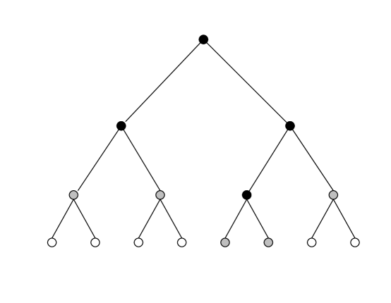
Figure 1: An Eden cluster of size $4$ on a Cayley tree. The black sites form the cluster and the shaded sites form the perimeter. At the next step, growth can occur at any of the $5$ shaded perimeter sites with equal probability $1/5$.

Fig. (2) shows all possible Eden clusters of size $3$ and their associated statistical weights.

Figure 2: All possible Eden clusters of size $3$ on a tree and their associated statistical weights w.

On the other hand, a binary search tree in computer science is constructed by the following simple algorithm Knuth ; Mahmoud ; Review . Imagine that we have a data string consisting of $N$ items which are labeled by the $N$ integers: $\{1,2,\dots,N\}$. These could be the months of the year or the names of people etc. Let us assume that this data appears in a particular order, say $\{6,4,5,8,9,1,2,10,3,7\}$ for $N=10$ integers. This data is first stored on a binary tree following the simple dynamical rule: the first item $6$ is stored at the root of the tree (see Fig. (3)). The next item in the string is $4$. We compare it with $6$ at the root and since $4<6$, we store $4$ in the left daughter node of the root. Had it been bigger than the root item $6$, we would have stored it in the right daughter node. The next item in the string is $5$. We again start from the root, see that $5<6$, so we go to the left branch. There we encounter $4$ and we find $5>4$, so we go the right daughter node of $4$. This process is continued till all the $N=10$ items are assigned their nodes and we get a unique binary search tree (BST) (see Fig. (3)) for this particular data string $\{6,4,5,8,9,1,2,10,3,7\}$.

Figure 3: The binary search tree associated with the data string $\{6,4,5,8,9,1,2,10,3,7\}$.

Usually the data arrives at a computer in random order. To study this situation, one considers the simplest model called the ‘random binary search tree’ (RBST) model where one assumes that the incoming data string can arrive in any of the $N!$ possible orders or sequences, each with equal probability Review . For each of these sequences, one has a binary tree. For example, in Fig. (4), we show the binary trees for $N=3$ along with their associated probabilities.

Figure 4: All possible random binary search trees for a data of size $N=3$ and their associated statistical weights.

Comparing Fig. (2) and Fig. (4), one sees immediately that the Eden trees after 3 steps have exactly the same configurations and statistical weights as the random binary search trees with data size $N=3$. This analogy can be easily extended to all $N$. The key point is that after $(n-1)$ steps there are $(n-1)$ occupied sites in the Eden cluster and $n$ perimeter sites (this is easy to understand as the addition of a new occupied site eliminates one old perimeter site while creating two new perimeter sites). The probability of subsequent growth at step $n$ at any of these perimeter sites is $p_{n}=1/n$. Thus the statistical weight of a cluster of $N$ sites formed by a specific history of growth is simply $w=p_{1}\,p_{2}\,\dots p_{N}=1/N!$, which is the same as in the RBST model. Thus the Eden model on the Cayley tree is exactly equivalent to the RBST.

Another popular search tree model is known as the ‘digital search tree’ (DST) which is constructed by the following rule Knuth ; Mahmoud ; Sedgewick ; FS ; Pittel ; FR ; KS ; SM1 . Consider again a binary Cayley tree each node of which can contain at most one entry. One starts with an empty tree and the data is stored sequentially. The first data item is stored in the root of the tree. The next one arrives at the root and finding it occupied, moves to any of the two empty daughter nodes chosen at random and occupies that node. Then the next item arrives and again it starts at the node, chooses any of its two daughters randomly and moves there. If the chosen daughter is empty it occupies it. If the chosen daughter is already occupied, it again chooses one of its two descendants at random and moves there. Thus at any stage, a new entry starts at the root and performs a random walk (to the left or to the right daughter with equal probability) down the tree till it finds an empty node and occupies the node. Thus one obtains again a growing tree where at any stage growth can occur at any of the perimeter sites, but now the growth probability at a perimeter site $a$ is $p_{a}\propto 2^{-l_{a}}$ where $l_{a}$ is the distance of the perimeter site from the root. The DST is an important tree structure in computer science and has been studied extensively. In particular, it turns out the DST is a natural tree representation AS ; KS of the data compression algorithm due to Ziv and Lempel LZ . Recently it was shown that a diffusion limited aggregation model introduced by Bradley and Strenski BS in physics is exactly equivalent the the DST model in computer science and a variety of exact results were obtained by exploiting this connection SM1 .

The examples above illustrate a profound link between growth models and the dynamics of search tree formation in computer science. Note that the two search tree models discussed above, the RBST and the DST, can be considered as special cases of a general growth model where growth occurs ( i.e. a new particle gets absorbed) at any of the available perimeter sites $a$ with a growth probability $p_{a}\propto c^{-l_{a}}$ where $c$ is a constant positive parameter and $l_{a}$ is the distance of the perimeter site $a$ from the root of the tree. The RBST (equivalently the Eden model) corresponds to $c=1$ so that all perimeter sites have equal probability to absorb a particle. The DST, on the other hand, corresponds to $c=2$ as discussed above. It is then useful and interesting to study this general growth model parametrized by $c$ and ask if there are any qualitative changes in the statistical properties of the growth clusters as one varies the parameter $c$ continuously. Indeed, Aldous and Shields studied a continuous-time version of this generalized growth model AS . Note that in the two models discussed above time is discrete and is equal to the number of particles in the tree. In the version of the model studied by Aldous and Shields, time is considered continuous and growth occurs at any of the available perimeter sites say the site $a$ with a rate proportional to $c^{-l_{a}}$ where $c$ is a positive parameter. In this continuous-time model, the total number of particles in the tree at time $t$ is thus a random variable, unlike in the discrete time version. Thus, while the discrete-time model has a constant particle number ensemble, the continuous-time model has a constant time ensemble, much like the canonical and the grand canonical ensemble in statistical physics. Asymptotically at long times, both the discrete-time and the continuous-time versions of the model are expected behave in a similar fashion. Henceforth, we will consider in this paper only the continuous-time version à la Aldous-Shields, since it is, from a technical point of view, easier to study than its discrete-time counterpart.

The question naturally arises whether the statistical properties of the growing clusters in this model undergo any qualitative change of behavior as one tunes the parameter $c$ continuously. Indeed, Aldous and Shields established rigorous probabilistic bounds to show that the nature of the fluctuations (variance) in the number of particles in the tree at time $t$ is qualitatively different for $c<\sqrt{2}$ and $c>\sqrt{2}$. While for $c>\sqrt{2}$ the central limit theorem holds and the total number of particles has a limiting Gaussian distribution AS , for $c<\sqrt{2}$ the central limit theorem breaks down due to the appearance of anomalously large fluctuations. Thus, there is a sharp phase transition in the nature of the fluctuations at a critical value $c=\sqrt{2}$. However, the mechanism responsible for this phase transition and even the explicit quantitative behavior of the fluctuations above, below, or at the critical point were not easy to obtain within the rigorous probabilistic analysis of Aldous and Shields. The principal purpose of this paper is to provide a detailed quantitative understanding of this rather ‘peculiar’ phase transition. Our method, completely different from the original approach of Aldous and Shields, employs a backward Fokker-Planck formalism. The advantage of this method is that one can obtain exact asymptotic results explicitly. Moreover, our analysis also shows that the mathematical mechanism behind this phase transition is similar to the phase transitions found recently in the variance of the number of nodes needed to store data on a $m$-ary search tree (where $m$ is the number of branches) at the critical value $m=26$ CH ; DM1 ; Review ; CP ; FN ; FFN ; TH and also in the variance of the number of splitting events in a $D$-dimensional fragmentation model at the critical value $D_{c}=\pi/{{\sin}^{-1}\left(1/\sqrt{8}\right)}=8.69363\ldots$ DM1 ; Review .

The layout of the paper is as follows. In the next Section (II), we define the model precisely and summarize the main results. We study here a generalized Aldous-Shields model where the growth takes place on a Cayley tree with $m$ branches. In Section III, we derive the evolution equations for the mean and variance of the number of occupied sites as a function of time via a backward Fokker Planck technique. A simple scaling analysis is then carried out to determine the temporal growth exponents. In Section IV a more thorough analysis of the evolution equations is provided that enables us to obtain explicitly not just the growth exponents, but also exact expressions for various amplitudes and prefactors that include interesting log-periodic oscillations. We conclude with a summary and a discussion of open questions in the last section.

II The Model and the Results

We consider a generalized Aldous-Shields model where growth occurs on a Cayley tree (rooted at $O$) with $m$ branches (see Fig. 5). Aldous and Shields studied AS only the binary case $m=2$. Initially the tree is empty and growth occurs in continuous time starting from the root $O$. At any instant $t$, one first identifies the available perimeter nodes. A node $a$ at time $t$ is a perimeter node if it is empty at $t$ but its parent node is occupied at $t$ (see Fig. 5). Subsequently, in a small time interval $\Delta t$, a perimeter node $a$ either absorbs a particle with probability $c^{-l_{a}}\,\Delta t$ or remains unoccupied with probability $(1-c^{-l_{a}}\,\Delta t)$, where $l_{a}$ is the depth of the perimeter node $a$, i.e. its distance from the root $O$. This growth process occurs simultaneously at all the perimeter nodes. Thus, the total number of particles $n(t)$ in the tree rooted at $O$ is clearly not a fixed number at a given time $t$, instead it is a random variable in the sense that the value of $n(t)$ differs from one history of evolution to another. We are interested in computing the statistics of $n(t)$ at large times $t$.

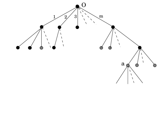
Figure 5: The growth of the Aldous-Shields model on a tree with $m$ branches and rooted at $O$. The filled circles are occupied nodes and the shaded ones are the perimeter nodes where growth can occur subsequently. For example the site marked $a$ is a typical perimeter site at a distance $l_{a}=3$ from the root $O$ of the tree.

In this model, we have two parameters $m$ and $c$. It is useful to first summarize our main results. Using a backward Fokker-Planck approach we derive an exact evolution equation for the generating function,

$$G(\mu,t)=\langle\exp\left(-\mu\,n(t)\right)\rangle=\sum_{n=0}^{\infty}e^{-\mu\,n}P(n,t)$$ (1)

where the angle brackets denote an average over all histories of the evolution process and $P(n,t)$ is the probability distribution of $n$ at time $t$. We show that $G(\mu,t)$ evolves via the equation

$$\frac{dG(\mu,t)}{dt}=-G(\mu,t)+e^{-\mu}\,G^{m}(\mu,t/c),$$ (2)

starting from the initial condition $G(\mu,0)=1$. By differentiating $G(\mu,t)$ with respect to $\mu$ and putting $\mu=0$, one can also derive the evolution equations for all the moments of $n(t)$. The equation (2) is nonlinear and nonlocal in time for generic values of $c$ and $m$, and is thus difficult to solve exactly, except for the $c=1$ case when it becomes local. However, we were able to compute exactly the asymptotic large time behaviors of the mean and the variance of $n(t)$ for arbitrary $m$ and $c$. Below we present our results for the three different cases $c=1$, $c<1$ and $c>1$ separately.

The case $c=1$: In this case our model is precisely the continuous-time version of the Eden model. This case $c=1$ is exactly solvable since the evolution equation (2) becomes local in time. We solved for $G(\mu,t)$ and obtained the following explicit result for the distribution $P(n,t)$ for all $m$ and $t$

$$P(n,t)=\frac{\Gamma\left(n+\frac{1}{m-1}\right)}{\Gamma\left(\frac{1}{m-1}\right)\,\Gamma(n+1)}\,e^{-t}\,\left[1-e^{-(m-1)\,t}\right]^{n}$$ (3)

where $\Gamma(x)$ is the standard Gamma function. The mean number of particles $M(t)=\langle n(t)\rangle$ increases exponentially in time for all $m>1$,

$$M(t)=\frac{1}{m-1}\left[\exp\left((m-1)t\right)-1\right].$$ (4)

For the special case $m=1$ (a line with a constant rate of deposition), $M(t)=t$ and the distribution $P(n,t)=e^{-t}t^{n}/{n}!$, obtained from Eq. (3) by taking the limit $m\to 1$, is purely Poissonian as expected.

The case $c<1$: Since the growth rate at a perimeter node $a$ is proportional to $c^{-l_{a}}$ where $l_{a}$ is the distance of the node from the root $O$, it is clear that for $c<1$, farther a perimeter node is from the root, the larger is its probability to get occupied. Thus the cluster grows in a rather ramified manner where long branches grow faster than the short branches. In this case we expect that the mean number of sites grows at least exponentially. But since physically this case is of little interest, we do not discuss it further in this paper.

The case $c>1$: We now come to the physically most relevant case $c>1$. We show that in this case there is a sharp phase transition in the asymptotic statistics of $n(t)$ across the critical line $c=\sqrt{m}$ in the $(m,c)$ plane with $m>1$ and $c>1$. We calculated exactly the asymptotic time dependence of the mean $M(t)=\langle n(t)\rangle$ and the variance $V(t)=\langle n^{2}(t)\rangle-M^{2}(t)$, for all values of $m>1$ and $c>1$. We show that while the fluctuations are normal (i.e. the variance of $n(t)$ is proportional to its mean) for $c>\sqrt{m}$, they are anomalously large for $c<\sqrt{m}$. Even though we have two parameters $c$ and $m$, it turns out that the asymptotic behaviors can be described in terms of the single growth parameter

$$\alpha=\frac{\ln(m)}{\ln(c)}$$ (5)

where $\alpha>0$ since $c>1$. In terms of $\alpha$, the phase transition takes phase at the critical value $\alpha_{c}=2$. The normal phase for $c>\sqrt{m}$ corresponds to $\alpha<\alpha_{c}=2$ and the anomalous phase for $c<\sqrt{m}$ corresponds to $\alpha>\alpha_{c}=2$.

Figure 6: The phase transition as a function of $\alpha=\ln(m)/\ln(c)>0$. The critical point at $\alpha_{c}=2$ separates the phase ($\alpha<2$) with normal fluctuations from the phase ($\alpha>2$) with anomalously large fluctuations.

More precisely, we find that for large $t$, the mean $M(t)$ grows as a power law (up to corrections periodic in $\ln(t)$),

$$M(t)\sim A\,t^{\alpha},$$ (6)

and we provide an explicit expression for the amplitude $A$. The variance, on the other hand, has different behaviors for $c<\sqrt{m}$ and $c>\sqrt{m}$ or equivalently for $\alpha>2$ and $\alpha<2$. We show that the variance at large times $t$, again up to log-periodic corrections, grows as

$$V(t) \simeq B^{\prime}\,t^{\alpha}\,\,\,\,\quad\quad\rm{for}\quad\quad\alpha<2$$ (7)

$$\simeq B_{c}\,t^{2}\ln(t)\,\,\,\rm{for}\quad\quad\alpha=\alpha_{c}=2$$ (8)

$$\simeq B\,t^{2\alpha-2}\,\,\,\,\quad\rm{for}\quad\quad\alpha>2.$$ (9)

We also provide exact expressions for the amplitudes $B^{\prime}$, $B_{c}$ and $B$. In order to use these continuous-time results for the discrete-time model where the ‘time’ is same as the number of particles, it is instructive to eliminate the explicit $t$ dependence in the results for the variance and instead express it as a function of the mean number of particles. Eliminating $t$ between Eqs. (6), (7), (8) and (9), we get

$$V(t) \sim C^{\prime}\,M(t)\,\,\,\quad\quad\rm{for}\quad\quad\alpha<2$$ (10)

$$\sim C_{c}\,M(t)\ln(M(t))\,\,\,\rm{for}\quad\alpha=\alpha_{c}=2$$ (11)

$$\sim C\,M(t)^{2-2/\alpha}\,\,\,\,\,\rm{for}\quad\quad\alpha>2.$$ (12)

Explicit expressions for the amplitudes $C^{\prime}$, $C_{c}$ and $C$ are likewise provided.

We thus see that for $\alpha<2$ the fluctuations of $n(t)$ about its mean value, denoted by $\Delta n(t)=\sqrt{V(t)}$, are of order $M^{1/2}$ as is the case for a normal Gaussian or Poisson distribution. However for $\alpha>2$ we find that $\Delta n(t)\sim M^{1-{1/\alpha}}$ for large $M$. For $\alpha>2$, we have that $1-{1/\alpha}>{1/2}$ and hence the relative fluctuations about the mean become larger as we cross the threshold $\alpha=2$ from below. The phase $\alpha<2$, or equivalently $c>\sqrt{m}$ corresponds to a region of slower growth where the central limit theorem holds and the distribution of $n(t)$ is asymptotically normal. On the other hand, $\alpha>2$ marks a phase where rapid growth tends to occur along a single branch resulting in anomalously large fluctuations. Thus the statistics of $n(t)$ in this phase is dominated by extreme fluctuations. The nature of this phase transition is thus very similar to the ones recently reported in $m$-ary search trees CH ; DM1 ; Review ; CP ; FN ; FFN ; TH and a related fragmentation model DM1 ; Review .

We end this section with a remark on the usage of the term ‘phase transition’. The ‘phase transition’ observed in this model refers to the abrupt change of the variance (and also that of the full distribution) of the number of particles $n(t)$ in the tree as one changes the parameter $\alpha=\ln(m)/\ln(c)$ through its critical value $\alpha_{c}=2$. This may not correspond to the traditional definition of ‘phase transition’ used in equilibrium statistical mechanics, e.g. the divergence of a correlation length as one approaches a critical point as in second order phase transition. The ‘phase transition’ in the Aldous-Shields model is closer to the change of behavior one observes in the diffusion of a Lévy walker. A Lévy walker jumps, at each step, by a random length $l$ drawn from a power law distribution, $p(l)\sim l^{-(1+\gamma)}$ for large $l$ with $\gamma>1$ (required for normalization). It is well knownBG that the root mean square displacement of the particle after $n$ steps $\sqrt{\langle R_{n}^{2}\rangle}\sim n^{1/2}$ for large $n$ only when $\gamma>2$, i.e. one gets normal diffusion and the asymptotic position of the walker is distributed normally. On the other hand, for $1<\gamma<2$ one gets anomalously large diffusion, $\sqrt{\langle R_{n}^{2}\rangle}\sim n^{1/\gamma}$ for large $n$ and the asymptotic distribution of the position of the walker is non-Gaussian. Thus there is a change of behavior at the critical value $\gamma_{c}=2$. The change of behavior in the variance of the number of particles in the Aldous-Shields model at the critical value $\alpha_{c}=2$ is thus similar in nature to the the change of behavior seen for the Lévy diffusion at $\gamma_{c}=2$, rather than the standard ‘phase transition’ observed in critical phenomena.

III Derivation of the evolution equations

In this section we will derive the evolution equation for the probability distribution, and in particular the evolution equations for the mean and the variance, of the total number of occupied sites $n(t)$ at time $t$ in a tree rooted at the site $O$. The root $O$, by definition, has level or depth $l_{0}=0$. The method of derivation is based on a backward Fokker Planck formalism which involves considering the future evolution of $n(t)$ conditioned on what happens in the first infinitesimal time interval $(0,\Delta t)$. Since our final aim is to derive a recursion relation for the evolution process, it is convenient to first derive the evolution equation for the number of particles $n_{a}(t)$ in a subtree rooted, say, at any arbitrary site $a$. By definition, $n_{a}(t)$ includes the particle at the root $a$. The number of particles in the full tree is just a special case when the site $a$ is chosen to be the original root $O$ of the full tree. We now count the ‘local’ time $t$ (for this subtree) from the instant the site $a$ becomes a potential growth site, so that, by definition, $n_{a}(0)=0$. Clearly, at any given $t$, the distribution $P(n_{a},t)$ of $n_{a}(t)$ depends only on $t$ and $l_{a}$, the depth of the site $a$. This means that one can write

$$\langle F(n_{a}(t))\rangle=\sum_{n_{a}=0}^{\infty}F(n_{a})\,P(n_{a},t)=f(t;l_{a})$$ (13)

where $F(x)$ is any arbitrary function.

Consider now the site $a$ with its descendants $a_{1},\ a_{2},\cdots,a_{m}$, where $a$ is a potential growth site at $t=0$. By definition $a$ is unoccupied at $t=0$ and thus $a_{1},\ a_{2},\cdots,a_{m}$ are not potential growth sites at $t=0$. In the first infinitesimal time interval $(0,\Delta t)$ there are two possibilities: (i) either no particle fills the potential growth site $a$, thus $n_{a}(t)=n_{a}(t-\Delta t)$. This happens with probability $1-c^{-l_{a}}\Delta t$. (ii) the other possibility is that the potential growth site $a$ is filled by a particle with probability $c^{-l_{a}}\Delta t$ and as a consequence the number of particles in the subtree rooted at $a$ is increased by one and the daughter nodes $a_{1},\ a_{2},\cdots,a_{m}$ all become potential growth sites. Mathematically we can write the above evolution in the following way: in the time interval $(0,\Delta t)$

$$n_{a}(t)=n_{a}(t-\Delta t)(1-I)+\left[1+\sum_{i=1}^{m}n_{a_{i}}(t-\Delta t)\right]I$$ (14)

where $I$ is a random variable which takes the value $1$ with probability $c^{-l_{a}}\Delta t$ and $0$ with probability $1-c^{-l_{a}}\Delta t$. Taking the expectation of Eq. (14) with respect to $I$ and the subsequent growth process in the remaining time $t-\Delta t$ we obtain, upon taking the limit $\Delta t\to 0$,

$$\frac{d}{dt}\langle n_{a}(t)\rangle=c^{-l_{a}}\left[1-\langle n_{a}(t)\rangle+\sum_{i=1}^{m}\langle n_{a_{i}}(t)\rangle\right].$$ (15)

We now use the property that the statistics of the number of particles in a subtree rooted at level $a$ depends only on $l_{a}$ as encoded in Eq. (13) to obtain

$$\frac{d}{dt}M(t;l_{a})=c^{-l_{a}}\left[1-M(t;l_{a})+mM(t;l_{a}+1)\right].$$ (16)

where we have defined

$$M(t;l_{a})=\langle n_{a}(t)\rangle$$ (17)

and have used the fact that by definition $l_{a_{i}}=l_{a}+1$ if $a_{i}$ is a daughter of the node $a$. Note that the root $O$ of the full tree has depth $l_{O}=0$. Thus the mean $M(t)=\langle n(t)\rangle$ of the total number of particles in the full tree rooted at $O$ is simply, $M(t)=M(t,0)$. Thus to obtain $M(t)$, our strategy is to find the solution $M(t,l_{a})$ of Eq. (16) for arbitrary $l_{a}$ and eventually put $l_{a}=0$.

The next step is to notice that as one goes down a level in the tree the growth rate is reduced by a factor of $c$ which amounts to rescaling time by a factor of $1/c$. In the notation of Eq. (13) this means that one may write

$$f(t;l_{a}+1)=f\left(\frac{t}{c};l_{a}\right).$$ (18)

Next we put $l_{a}=0$ in Eq. (16), use the definition $M(t;l_{O})=M(t;0)=M(t)$ and also the scaling property in Eq. (18) to obtain,

$$\frac{d}{dt}M(t)=1-M(t)+mM\left(\frac{t}{c}\right).$$ (19)

This equation, supplemented by the boundary condition $M(0)=0$, then describes the evolution of the mean number of occupied sites.

An equation for the variance of $n(t)$ can be derived in a similar fashion. The starting point is obtained by squaring the stochastic evolution equation (14) and then taking the expectation over $I$ and the evolution in the remaining time $t-\Delta t$. This yields

$$\langle n^{2}_{a}(t)\rangle=\langle n^{2}_{a}(t-\Delta t)\rangle(1-c^{-l_{a}}\Delta t)+\left[1+2\langle\sum_{i=1}^{m}n_{a_{i}}(t-\Delta t)\rangle+\langle\left(\sum_{i=1}^{m}n_{a_{i}}(t-\Delta t)\right)^{2}\rangle\right]c^{-l_{a}}\Delta t.$$ (20)

We now use the fact that the subtrees rooted at sites at the same level are statistically independent and so

$$\langle n_{a_{i}}(t)n_{a_{j}}(t)\rangle=\langle n_{a_{i}}(t)\rangle\langle n_{a_{j}}(t)\rangle\ {\rm{for}}\ i\neq j.$$ (21)

Now defining the variance of the number of sites occupied in the tree rooted at $0$ as

$$V(t)=\langle n^{2}(t)\rangle-\langle n(t)\rangle^{2}$$ (22)

and using the scaling relation Eq. (18), after some elementary algebra, we obtain

$$\frac{d}{dt}V(t)=\left(\frac{d}{dt}M(t)\right)^{2}-V(t)+mV\left(\frac{t}{c}\right).$$ (23)

The boundary condition for this equation is clearly $V(0)=0$.

Another way to obtain the equations for $M$ and $V$ is by deriving directly an evolution equation for the generating function $G(\mu,t)$ of $n(t)$ defined as in Eq. (1). Following exactly the same backward Fokker-Planck strategy as used for the mean, it is straightforward to show that $G(\mu,t)$ evolves by the nonlinear nonlocal equation (2). The moment equations, and equations for the higher moments, Eq. (19) and Eq. (23) can be obtained by differentiating Eq. (2) with respect to $\mu$ the appropriate number of times and setting $\mu=0$ at the end.

The evolution equation (2) is difficult to solve explicitly for generic values of $c$ and $m$ since it is a nonlinear (for $m\neq 1$) and nonlocal (for $c\neq 1$) equation. However, exact results can be derived in a few cases that we consider below. The asymptotic solution for the mean and variance for generic $m$ and $c$ will be presented later in the next section.

III.1 Exact Solution for the Eden Growth $c=1$

The case $c=1$ corresponds to the Eden model where growth occurs at any of the available perimeter sites with equal rates. For $c=1$, Eq. (2) becomes local in time $t$ and can be explicitly solved. We find that for all $m\geq 1$

$$G(\mu,t)=e^{-t}\,\left[1-e^{-\mu}\,\left(1-e^{-(m-1)t}\right)\right]^{-1/(m-1)}.$$ (24)

Expanding the r.h.s. of Eq. (24) in powers of $e^{-\mu}$ as in Eq. (1), one can then read off the distribution $P(n,t)$ explicitly as in Eq. (3). The mean number of particles grows exponentially for all $m>1$ as in Eq. (4). Similarly, one can compute the variance $V(t)$. We find

$$V(t)=\frac{1}{(m-1)}\,e^{(m-1)t}\left(e^{(m-1)t}-1\right)\,.$$ (25)

For a fixed $m$, if one takes the limit of large $t$ and large $n$ keeping the product $n\,e^{-(m-1)t}$ fixed in Eq. (3), one finds an asymptotic distribution

$$P(n,t)\simeq\frac{e^{-t}}{\Gamma\left(\frac{1}{(m-1)}\right)}\,n^{-(m-2)/(m-1)}\,\exp\left[-n\,e^{-(m-1)t}\right].$$ (26)

Thus, to the leading order, the distribution $P(n,t)$ decays exponentially for large $n$ over a characteristic size $n^{*}\sim e^{(m-1)t}$ that grows exponentially with time $t$. Interestingly, the distribution has a sub-leading power law tail (in addition to the leading exponential tail) $n^{-\phi}$ where the exponent $\phi=(m-2)/(m-1)$ depends continuously on $m$.

For the special case $m=1$, where we have just a line of sites and the particles arrive at an empty available site at a constant rate $1$, we get from Eq. (4), $M(t)=t$. The full distribution, from Eq. (3), becomes a Poisson distribution $P(n,t)=e^{-t}t^{n}/{n!}$ as expected.

III.2 Exact Solution for the Digital Search Tree Growth $c=m$

The case $c=m$ corresponds to the case where particles arrive at a constant rate at the root $O$ and then each carries out a random walk down the tree until it finds a free site to occupy. During its downward journey in the tree the particle, after arriving at any occupied site, chooses one of its $m$ descendants at random. This is precisely the algorithm for constructing a $m$-ary digital search tree Knuth ; Sedgewick ; AS . If the rate at which the particles arrive at the root $O$ is one then the total number of particles in the tree at time $t$, $n(t)$, is clearly a random variable with Poisson distribution

$$P(n=k,t)=\frac{t^{k}\exp(-t)}{k!},$$ (27)

where $k=0,1,2\cdots$ is a positive integer. This yields

$$M(t)=t;\ V(t)=t,$$ (28)

which we see immediately are the solutions to Eq (19) and Eq. (23). Furthermore we see that the generating function $G(\mu,t)$ for a Poisson distribution is given by

$$G(t,\mu)=\exp\left(-t+t\exp(-\mu)\right).$$ (29)

It is easy to check that indeed this solves Eq. (2) in the case $m=c$.

III.3 A self-consistent scaling approach for the leading asymptotic growth of the mean and the variance for $c>1$ and $m>1$

The late time asymptotic behavior of Eq. (19) and Eq. (23) for $c>1$ and $m>1$ may be deduced quite simply by making a self-consistent ansatz for the late time behavior of $M$ and $V$. First consider Eq. (19). We make the ansatz

$$M(t)\simeq A\,t^{\alpha}.$$ (30)

Substituting this into Eq. (19) we may neglect the derivative term on the l.h.s. and assuming that $\alpha>0$ (i.e. $c>1$), matching the coefficients of $t^{\alpha}$ gives

$$\frac{m}{c^{\alpha}}-1=0,$$ (31)

which yields

$$\alpha=\frac{\ln(m)}{\ln(c)}.$$ (32)

For non-trivial tree structures we are always in the situation where $m\geq 2$ and for the above solution to make sense we require that $c>1$ to have a positive exponent $\alpha$. While this simple minded scaling approach yields the correct power law growth of $M(t)\simeq A\,t^{\alpha}$ for $c>1$, it does not provide us the value of the amplitude $A$. To derive an exact expression for $A$, we need to solve the full nonlocal equation (19) at late times, and this will be carried out in the next section.

Let us make a similar power law ansatz for the late time behavior of $V(t)$

$$V(t)\simeq B\,t^{\beta}.$$ (33)

Substituting this into Eq. (23) and neglecting the derivative term we obtain

$$-Bt^{\beta}+Bm\frac{t^{\beta}}{c^{\beta}}+A^{2}\alpha^{2}t^{2\alpha-2}=0.$$ (34)

Asymptotically there are two ways to satisfy this equation. First if we assume a priori that $\beta>2\alpha-2$ then the first two terms in Eq. (34) must cancel leading to $c^{\beta}=m$, i.e. $\beta=\ln(m)/\ln(c)=\alpha$. The a posteriori condition that this solution is valid is thus $\alpha>2\alpha-2$, which means $\alpha<2$. The second possibility is that all three terms contribute and thus $\beta=2\alpha-2$. In this case we find that

$$B=\frac{A^{2}\alpha^{2}}{1-\frac{m}{c^{2\alpha-2}}}=\frac{A^{2}\alpha^{2}}{1-c^{2-\alpha}},$$ (35)

and in obtaining the last equality in Eq. (35) we have used $m=c^{\alpha}$. However for this solution to make sense we must have that $B>0$ because $V(t)$ is clearly positive, consequently Eq. (35) can only hold when $\alpha>2$ (since $c>1$).

This simple minded scaling approach thus indicates that there is a phase transition in the late time behavior of the variance $V(t)$ at the critical parameter value $\alpha_{c}=2$. For $\alpha<2$, we have $V(t)\sim B^{\prime}\,t^{\alpha}$ where the amplitude $B^{\prime}$ can not be determined by the scaling approach. On the other hand, for $\alpha>2$ the scaling approach indicates $V(t)\sim B\,t^{2\alpha-2}$ and moreover it provides a relationship between the amplitudes $B$ and $A$ (of the mean) via Eq. (35). The critical point $\alpha_{c}=2$ thus separates the region of normal growth $\alpha<2$ (or equivalently $c>\sqrt{m}$), where $V(t)\sim M(t)$, from the the region $\alpha>2$ (i.e. $c<\sqrt{m}$) where the variance grows anomalously faster $V(t)\sim[M(t)]^{2-2/\alpha}$. In the next section, we will see that the analysis of the full nonlocal equations (19) and (23) indeed corroborates theses scaling results, and in addition produces exact expressions for all the amplitudes.

Before proceeding to the full analysis of Eqs. (19) and (23) in the next section for generic $c>1$ and $m$, it is instructive to note that analytic progress is also possible for Eq. (19) in the case where $\alpha=\ln(m)/\ln(c)$ is a positive integer. This includes, in particular, the critical point $\alpha=2$. We make the following ansatz

$$M(t)=\sum_{k=1}^{\infty}b_{n}t^{n},$$ (36)

where the term $k=0$ in the above sum is omitted in order to respect the initial condition $M(0)=0$. Matching powers of $t$ on substituting this ansatz into Eq. (19) yields

$$b_{1} = 1$$

$$b_{k+1} = b_{k}\frac{1}{k+1}\left(\frac{m}{c^{k}}-1\right)\ {\rm for}\quad k>1.$$ (37)

We thus see that if there exists a positive integer $k^{*}$ such that $\alpha=\ln(m)/\ln(c)=k^{*}$ then $b_{k}=0$ for all $k>k^{*}=\alpha$ and we have found the solution to Eq. (19) in these cases. At late times the leading order behavior is thus dominated by the term containing $t^{\alpha}$ and we get

$$M(t) \sim \frac{t^{\alpha}}{\alpha!}\left(\frac{m}{c^{\alpha-1}}-1\right)\left(\frac{m}{c^{\alpha-2}}-1\right)\cdots\left(\frac{m}{c}-1\right)$$ (38)

$$= \frac{t^{\alpha}}{\alpha!}\left({c}^{\alpha-1}-1\right)\left({c}^{\alpha-2}-1\right)\cdots\left({c}-1\right).$$

In particular, at the critical point $\alpha=2$, we get for large $t$

$$M(t)\simeq\frac{(c-1)}{2}\,t^{2}$$ (39)

Thus, at this special point $\alpha=2$, we have even managed to compute the amplitude $A=(c-1)/2$ of the mean $M(t)\sim A\,t^{2}$ exactly. In the case $\alpha>2$, the behavior of the variance $V(t)$ now follows immediately from Eq. (35). Finally, exactly at the critical point $\alpha=2$, we may asymptotically solve Eq. (23) with the ansatz $V=B\,t^{2}\ln(t)$ to yield

$$B=\frac{4}{\ln(c)}A^{2}=\frac{(c-1)^{2}}{\ln(c)},$$ (40)

where in the last line of Eq. (40) we have used $A=(c-1)/2$.

IV General solution of the evolution equations of the Mean and the Variance

The full solutions to the nonlocal and nonlinear differential equations of the type in Eqs. (19,23) are rather difficult to obtain completely. Here we obtain the exact asymptotic solutions following an approach similar to the one used by Flajolet and Richmond  FR in solving a class of difference-differential equations arising in the context of digital search trees.

IV.1 Solution for the mean $M(t)$

We start by the analysis of Eq. (19) assuming $c>1$ and $m>1$. Taking the Laplace transform of Eq. (19) we obtain

$$s{\tilde{M}}(s)=\frac{1}{s}-{\tilde{M}}(s)+mc{\tilde{M}}(cs),$$ (41)

where

$${\tilde{M}}(s)=\int_{0}^{\infty}dt\ \exp(-st)M(t)$$ (42)

and we have used the initial condition $M(0)=0$. The above may be written as

$${\tilde{M}}(s)=\frac{1}{s(s+1)}+\frac{mc}{(s+1)}{\tilde{M}}(cs).$$ (43)

Now as ${\tilde{M}}(s)$ should go to zero as $s\to\infty$ and we are considering the case $c>1$, we solve Eq. (43) by iteration finding

$${\tilde{M}}(s)=\frac{1}{s}\sum_{j=0}^{\infty}\frac{m^{j}}{(1+s)(1+cs)\cdots(1+c^{j}s)}.$$ (44)

Note that taking the limit $s\to 0$ is not straightforward in Eq. (44). This is because if we set $s=0$ in the sum on the r.h.s of Eq. (44), the sum diverges since $m>1$. Following FR we introduce the function

$$Q(u)=\prod_{l=0}^{\infty}\left(1+\frac{u}{c^{l}}\right).$$ (45)

Thus $Q(s/c)=(1+s/c)(1+s/c^{2})(1+s/c^{3})\ldots$. On the other hand,

$$Q(c^{j}s)=\prod_{j=0}^{\infty}(1+c^{j-l}s) = (1+c^{j}s)(1+c^{j-1}s)\cdots(1+cs)(1+s)(1+s/c)(1+s/c^{2})\ldots$$ (46)

$$= (1+s)(1+cs)(1+c^{2}s)\cdots(1+c^{j}s)Q(s/c).$$

Thus, one can rewrite the product $(1+s)(1+cs)\cdots(1+c^{j}s)=Q(c^{j}s)/Q(s/c)$. Using this in Eq. (44) we get

$${\tilde{M}}(s)=\frac{Q({s/c})}{s}\ H(s),$$ (47)

where

$$H(s)=\sum_{j=0}^{\infty}\frac{m^{j}}{Q(c^{j}s)}.$$ (48)

The next step is to take the Mellin transform of $H(s)$ defined as

$$H^{*}(x)=\int_{0}^{\infty}ds\ s^{x-1}\ H(s).$$ (49)

Substituting $H(s)$ from Eq. (48) in the definition in Eq. (49) we get

$$H^{*}(x) = \sum_{j=0}^{\infty}m^{j}\int_{0}^{\infty}\frac{s^{x-1}}{Q(c^{j}s)}ds$$ (50)

$$= \sum_{j=0}^{\infty}(mc^{-x})^{j}\int_{0}^{\infty}\frac{\sigma^{x-1}}{Q(\sigma)}\,d\sigma$$

$$= \frac{h^{*}(x)}{1-mc^{-x}},$$

where

$$h^{*}(x)=\int_{0}^{\infty}d\sigma\ \frac{\sigma^{x-1}}{Q(\sigma)}$$ (51)

and in evaluating the sum over $j$ we have assumed ${\rm Re}(mc^{-x}<1)$ or equivalently ${\rm Re}(x)>\ln(m)/\ln(c)=\alpha$. We also notice that $h^{*}(x)$ has no poles for ${\rm Re}(x)>0$, and that the poles of $1/(1-mc^{-x})$ are at $x_{k}=\alpha+2\pi ik/\ln(c)$ where $k=0,\pm 1,\pm 2,\ldots$ runs over all integers. All the poles of $H^{*}(x)$ are thus to the left of the line ${\rm Re}(x)=\alpha$.

The inversion formula for the Mellin transform is given by

$$H(s)={1\over 2\pi i}\int_{-i\infty+d}^{i\infty+d}dx\ H^{*}(x)s^{-x},$$ (52)

where the above limits denote an integration up the imaginary axis to the right of all the poles of $H^{*}$, therefore we chose limits with $d>\alpha$. The contour may be closed in the left half plane (we assume that the integrand vanishes in the region ${\rm Re}(x)\to-\infty$) and we can thus evaluate the inverse Mellin transform in terms of the residues of the poles to the left of ${\rm Re}(x)\leq\alpha$, i.e

$$H(s)=\sum_{\rm{poles}}{\rm Res}\left[\frac{h^{*}(x)s^{-x}}{1-\exp\left(\ln(m)-x\ln(c)\right)}\right]$$ (53)

where $\rm{Res}$ denotes the residue at the pole in question.

The large time behavior of $M(t)$ is determined by the small $s$ behavior of ${\tilde{M}}(s)$. Now at small $s$ the dominant behavior clearly comes from the poles $x_{k}=\alpha+2\pi ik/\ln(c)$ running up the imaginary axis, any pole coming to the left of this line of poles will be higher order in $s$. We evaluate the residues in Eq. (53), substitute the resulting $H(s)$ in Eq. (47) and then take the limit $s\to 0$ to obtain the following asymptotic result

$${\tilde{M}}(s)\sim\frac{1}{s^{\alpha+1}\ln(c)}\left[h^{*}(\alpha)+\sum_{k\neq 0}h^{*}(\alpha+2\pi ik/\ln(c))s^{\frac{2\pi ik}{\ln(c)}}\right],$$ (54)

where we have used the fact $Q(0)=1$. Note that from Eq. (51) and Eq. (45), we have

$$h^{*}(\alpha)=\int_{0}^{\infty}\frac{\sigma^{\alpha-1}\,d\sigma}{(1+\sigma)(1+\sigma/c)(1+\sigma/c^{2})\ldots}=\frac{\pi}{\sin(\pi\alpha)}\prod_{k=1}^{\infty}\frac{1-c^{\alpha-k}}{1-c^{-k}},$$ (55)

where the last equality follows from an identity due to Ramanujan ram . Note that this identity explicitly shows that the function $h^{*}(x)$ has simple poles at the negative integers and zero but no poles for ${\rm Re}(x)>0$ as was stated before.

To extract the leading asymptotic behavior of $M(t)$ for large $t$, let us first divide the Laplace transform ${\tilde{M}}(s)$ into two parts, ${\tilde{M}}(s)={\tilde{M}_{p}}(s)+{\tilde{M}_{l}}(s)$ where ${\tilde{M}_{p}}(s)$ denote the first term on the r.h.s. of Eq. (54) and ${\tilde{M}_{l}}(s)$ corresponds to the remaining sum over $k\neq 0$. Subsequently the inverse Laplace transform $M(t)=M_{p}(t)+M_{l}(t)$ can also be divided into two parts. The term ${\tilde{M}_{p}}(s)$ has a pure algebraic form, thus its inverse $M_{p}(t)$ has a pure power law growth,

$$M_{p}(t)\sim A\ t^{\alpha},$$ (56)

where the constant $A$ can be evaluated as follows. If $M_{p}(t)$ has the form in Eq. (56), its Laplace transform is ${\tilde{M}_{p}}(s)=A\,\Gamma(1+\alpha)\,s^{-(1+\alpha)}$. Comparing this with the first term in Eq. (54) gives

$$A=\frac{h^{*}(\alpha)}{\ln(c)\Gamma(1+\alpha)}=\frac{\pi}{\ln(m)\Gamma(\alpha)\sin(\pi\alpha)}\prod_{k=1}^{\infty}\frac{1-c^{\alpha-k}}{1-c^{-k}},$$ (57)

where we have used $\Gamma(1+\alpha)=\alpha\Gamma(\alpha)$, the definition $\alpha=\ln(m)/\ln(c)$ and the explicit form of $h^{*}(\alpha)$ from Eq. (55). Here we note that when $\alpha$ is an integer, it can be verified that Eq. (57) agrees with Eq. (38) derived for discrete values of $\alpha$ in the previous section.

The second contribution to ${\tilde{M}}(s)$, $\tilde{M}_{l}(s)$ is given by a Fourier series in $\ln(s)$. The inverse Laplace transform of this term is difficult to obtain fully but it is easy to see that it gives rise to a late time behavior of the form

$$M_{l}(t)\sim{A\,t^{\alpha}}g\left(\ln(t)\right)$$ (58)

where $g(x)$ is a periodic function of $x$. The final asymptotic result for large $t$ is thus

$$M(t)=M_{p}(t)+M_{l}(t)\simeq{A\,t^{\alpha}}\left[1+g\left(\ln(t)\right)\right].$$ (59)

This exact result thus not only confirms the dominant power-law scaling predicted in section (III) up to log-periodic oscillations, but also provides an explicit formula for the amplitude $A$ as in Eq. (57). For example, let us consider the binary case $m=2$. For the case, when $c=1$, the formula in Eq. (57) gives $A=1$, thus $M(t)\simeq t$ for large $t$. On the other hand, for $m=2$, when $c=\sqrt{2}$ (the critical point), one can show from Eq. (57) that $A=(\sqrt{2}-1)/2$ and $M(t)\simeq(\sqrt{2}-1)t^{2}/2$ for large $t$.

IV.2 Solution for the variance $V(t)$

We now examine the asymptotic behavior of the variance $V(t)$ for large $t$ using a similar formalism. The evolution equation (23) for the variance $V(t)$ is similar to that for the mean $M(t)$ in Eq. (19) except that the source term in Eq. (23) is $(dM/dt)^{2}$, different from the source term $1$ in Eq. (19). Solution of Eq. (23) thus requires an explicit knowledge of how $M(t)$ behaves with time. Taking the Laplace transform, ${\tilde{V}}(s)=\int_{0}^{\infty}V(t)e^{-st}\,dt$ in Eq. (23) and using $V(0)=0$ we obtain

$$s{\tilde{V}}(s)=S(s)-{\tilde{V}}(s)+mc{\tilde{V}}(cs),$$ (60)

where

$$S(s)=\int_{0}^{\infty}dt\exp(-st)\left(\frac{dM}{dt}\right)^{2}.$$ (61)

Rearranging Eq. (60) gives

$${\tilde{V}}(s)=\frac{S(s)}{1+s}+\frac{mc}{1+s}\,{\tilde{V}}(cs)$$ (62)

which can be iterated to yield

$${\tilde{V}}(s)=\sum_{j=0}^{\infty}\frac{(mc)^{j}}{(1+s)(1+cs)\cdots(1+c^{j}s)}\,S(c^{j}s).$$ (63)

Using $m=c^{\alpha}$ and the function $Q(u)$ defined in Eq. (45) we can rewrite Eq. (63) as

$${\tilde{V}}(s)=Q(s/c)H_{1}(s)$$ (64)

where

$$H_{1}(s)=\sum_{j=0}^{\infty}\left(c^{1+\alpha}\right)^{j}\frac{S(c^{j}s)}{Q(c^{j}s)}.$$ (65)

The next step is to take the Mellin transform $H_{1}^{*}(x)=\int_{0}^{\infty}H_{1}(s)s^{x-1}ds$ of Eq. (65) which gives, after a change of variable $c^{j}s\to s$ in the integration

$$H_{1}^{*}(x)=\sum_{j=0}^{\infty}\left(c^{1+\alpha-x}\right)^{j}\int_{0}^{\infty}\frac{S(s)}{Q(s)}s^{x-1}ds.$$ (66)

Let us first assume that the integral

$$h_{1}^{*}(x)=\int_{0}^{\infty}\frac{S(s)}{Q(s)}s^{x-1}ds$$ (67)

exists (the conditions for which will be stated later). Then, for ${\rm Re}(x)>1+\alpha$, the geometric sum in Eq. (66) converges (since $c>1$) and we get

$$H_{1}^{*}(x)=\frac{h_{1}^{*}(x)}{1-c^{1+\alpha-x}}.$$ (68)

Inverting this Mellin transform we get

$$H_{1}(s)=\frac{1}{2\pi i}\int_{-i\infty+d}^{i\infty+d}\frac{h_{1}^{*}(x)}{1-c^{1+\alpha-x}}s^{-x}dx=\sum_{\rm poles}{\rm Res}\left[\frac{h_{1}^{*}(x)}{1-c^{1+\alpha-x}}s^{-x}\right],$$ (69)

where the poles are at $x_{k}=1+\alpha-2\pi ik/{\ln(c)}$ with $k=0,\pm 1,\pm 2,\ldots$. In Eq. (69) the integration is along the imaginary axis to the right of all the poles and then we close the contour over the left half plane. Evaluating the residues and substituting the results in Eq. (64) we get

$${\tilde{V}}(s)=\frac{Q(s/c)}{s^{1+\alpha}\ln(c)}\left[h_{1}^{*}(1+\alpha)+\sum_{k\neq 0}h_{1}^{*}\left(1+\alpha-2\pi ik/\ln(c)\right)\right],$$ (70)

where $h_{1}^{*}(x)$ is given by Eq. (67) assuming that it exists.

We now need to invert the Laplace transform in Eq. (70) to evaluate $V(t)$. For large $t$, as usual, the dominant contribution will come from the small $s$ behavior of ${\tilde{V}}(s)$. Using $Q(0)=1$ and assuming $h_{1}^{*}(1+\alpha-2\pi ik/\ln(c))$ exists for all $k=0,\pm 1,\pm 2\ldots$, it is clear from the small $s$ behavior of ${\tilde{V}}(s)$ in Eq. (70) that for large $t$

$$V(t)\simeq B^{\prime}\,t^{\alpha}[1+G(\ln(t))],$$ (71)

where $G(x)$ is a periodic function in $x$ and the amplitude $B^{\prime}$ can be read off as

$$B^{\prime}=\frac{h_{1}^{*}(1+\alpha)}{\Gamma(1+\alpha)\ln(c)};\,\,\,{\rm where}\,\,\,\,h_{1}^{*}(1+\alpha)=\int_{0}^{\infty}\frac{S(s)}{Q(s)}s^{\alpha}ds.$$ (72)

Having obtained the results in Eqs. (71) and (72), we need to investigate when they are valid. These results are valid as long as the integral $h_{1}^{*}(1+\alpha)$ in Eq. (72) exists. The existence of this integral depends on the small $s$ behavior of the source function $S(s)$ defined in Eq. (61). Using the asymptotic behavior of $M(t)$ from Eq. (59) we find that for large $t$

$$\left(\frac{dM}{dt}\right)^{2}\simeq A^{2}\alpha^{2}t^{2\alpha-2}\left[1+g_{1}(\ln(t)\right],$$ (73)

where $g_{1}(x)$ is a periodic function in $x$. Substituting this large $t$ behavior of $(dM/dt)^{2}$ in Eq. (61), it follows that, in the case $\alpha<1/2$, the integral converges to a nonzero constant as $s\to 0$. On the other hand, for $\alpha>1/2$, the integral diverges as $S(s)\simeq A^{2}\alpha^{2}\Gamma(2\alpha-1)s^{-(2\alpha-1)}$ as $s\to 0$. Up to the log-periodic oscillations, the leading behavior of $S(s)$ for small $s$ can be summarized as follows

$$S(s) \simeq C_{0}s^{-(2\alpha-1)}\,\,\,\quad{\rm for}\quad\quad\alpha>1/2$$ (74)

$$\simeq -\ln(s)\,\,\,\quad{\rm for}\quad\quad\alpha=1/2$$ (75)

$$\simeq A_{1}\,\,\,\quad\quad{\rm for}\quad\quad\alpha<1/2$$ (76)

where

$$C_{0}=A^{2}\alpha^{2}\Gamma(2\alpha-1)$$ (77)

is a positive constant for $\alpha>1/2$. Also, $A_{1}=\int_{0}^{\infty}(dM/dt)^{2}dt$ is a constant that depends on the full form of $M(t)$ and not just on its asymptotic behavior since for $\alpha<1/2$ the integral is convergent. Substituting this small $s$ behavior of $S(s)$ into the integral giving $h_{1}^{*}(1+\alpha)$ in Eq. (72) and using $Q(0)=1$, it is clear that the integral exists (no divergence from the small $s$ limit) only for $\alpha<2$. For $\alpha>2$, the integral does not exist since the integrand for small $s$ scales as $s^{1-\alpha}$. Thus the results in Eqs. (71) and (72) hold only for $\alpha<2$.

For $\alpha>2$, the above analysis breaks down and we need to employ a different method. We now go back to our starting equations (64) and (65). It turns out that for $\alpha>2$, we can actually extract the leading small $s$ behavior directly from these two equations. We directly substitute in Eq. (65) the leading small $s$ behavior of $S(s)\simeq C_{0}s^{-(2\alpha-1)}$ from Eq. (74) where $C_{0}=A^{2}\alpha^{2}\Gamma(2\alpha-1)$. Additionally we use $Q(0)=1$. Eqs. (64) and (65) then yield in the $s\to 0$ limit

$${\tilde{V}}(s)\simeq\frac{C_{0}}{s^{2\alpha-1}}\sum_{j=0}^{\infty}\left(c^{2-\alpha}\right)^{j}=\frac{C_{0}}{s^{2\alpha-1}(1-c^{2-\alpha})}$$ (78)

where we have used $\alpha>2$ which ensures that the sum in Eq. (78) is convergent. Inverting the Laplace transform, we then get the large $t$ behavior of $V(t)$ for $\alpha>2$

$$V(t)\simeq B\,t^{2\alpha-2};\,\,\,\,{\rm where}\,\,\,\,B=\frac{\alpha^{2}A^{2}}{1-c^{2-\alpha}},$$ (79)

where the constant $A$ is given in Eq. (57). Note that this result in Eq. (79) for $\alpha>2$ is in perfect agreement with the self-consistent scaling approach used in Section-III.

At the critical point $\alpha=2$, the analysis is more delicate. However, from the scaling approach of Section-III, we already know that for large $t$, $V(t)\simeq B_{c}\,t^{2}\ln(t)$ with $B_{c}=(c-1)^{2}/\ln(c)$ as in Eq. (40). Thus, the asymptotic behavior of the variance $V(t)$ can be summarized as

$$V(t) \simeq B^{\prime}\,t^{\alpha}\,\,\,\quad\rm{for}\quad\alpha<2$$ (80)

$$\simeq B_{c}\,t^{2}\ln(t)\,\,\,\quad\rm{for}\quad\alpha=\alpha_{c}=2$$ (81)

$$\simeq B\,t^{2\alpha-2}\,\,\,\,\,\quad\rm{for}\quad\alpha>2,$$ (82)

where the three amplitudes are given by

$$B^{\prime} = \frac{1}{\Gamma(1+\alpha)\ln(c)}\int_{0}^{\infty}\frac{S(s)}{Q(s)}s^{\alpha}ds$$

$$B_{c} = (c-1)^{2}/{\ln(c)}$$

$$B = \frac{\alpha^{2}A^{2}}{1-c^{2-\alpha}}$$ (83)

where $A$ is given in Eq. (57). Note that computing the amplitude $B^{\prime}$ explicitly requires an integration over the full source function $S(s)$ which is not so easy. Eliminating the time $t$ between $M(t)\simeq A\,t^{\alpha}$ and $V(t)$ in Eq. (82), one can express the variance $V$ as a function of the mean $M$ for large $M$ as in Eqs. (10), (11) and (12) and one can read off the constants $C^{\prime}$, $C_{c}$ and $C$ in terms of $B^{\prime}$, $B_{c}$ and $B$ and the amplitude $A$ of the mean given in Eq. (57).

Let us end this section with a remark on the mathematical mechanism responsible for the phase transition in the variance of the number of particles in this Aldous-Shields model. We note that the exact evolution equations (19) and (23) respectively for the mean and the variance are very similar—they are both linear and nonlocal in time, the only difference is in the source term. For the mean $M(t)$ in Eq. (19), the source term is a constant $1$ (the first term on the r.h.s of Eq. (19)). On the other hand, for the variance, the source term $(dM/dt)^{2}$ in Eq. (23) depends on the evolution of the mean. Thus, the mean feeds into the variance equation as an external source term leading to a competition between the growth induced by this external source term and the growth induced internally by the remaining two terms on the r.h.s of Eq. (23). This competition between the external and the internal source is finally responsible for the phase transition in the asymptotic growth of $V(t)$. For $\alpha<2$, the internal source term wins out and the variance grows similarly as the mean, $V(t)\sim M(t)\sim t^{\alpha}$, leading to the normal phase. On the other hand, for $\alpha>2$, the external source term wins out leading to a faster growth $V(t)\sim t^{2\alpha-2}\sim[M(t)]^{2-2/\alpha}$ characterizing anomalously large fluctuations. We note that a similar mechanism namely a “competition between the internal source and the external driving” was shown to be responsible for phase transitions in fluctuations in a class of fragmentation problems studied recentlyDM1 ; Review . In these fragmentation problems, it was shown that the mean and the variance evolved via similar looking equationsDM1 ; Review , except that they differed in their respective source terms—the variance equation had a source term driven by the mean, in much the same way as in the Aldous-Shields model discussed here. Thus, it seems that this phase transition in fluctuations is quite generic as it occurs in a large class of problems and the mathematical mechanism responsible for it is as identified above.

V Summary and Conclusion

In this paper we have studied analytically a growing tree model introduced by Aldous and Shields. In this model, growth occurs in continuous time. One starts at $t=0$ with an empty Cayley tree with $m$ branches rooted at $0$ and the tree grows, starting from the root site, by absorbing particles in continuous time. Each site can occupy at most one particle. At a given instant $t$, growth can occur only at the perimeter sites with a rate $c^{-l}$ where $c$ is positive parameter and $l$ is the distance of the perimeter site from the root of the tree. For $c=1$ this model is isomorphic to a continuous-time Eden model on a tree and also corresponds to the random binary search tree problem in computer science. For $c=2$ this model corresponds to the digital search tree problem in computer science.

We have introduced a backward Fokker-Planck approach that enabled us to study analytically the statistics of the total number of particles $n(t)$ in the tree at large time $t$. We have shown that at large $t$, while the mean number of particles grows as a power law in time, $M(t)\simeq A\,t^{\alpha}$ with $\alpha=\ln(m)/\ln(c)$ for all $c>1$, the variance $V(t)$ of the number of particles has two different behaviors depending on the value of the parameter $\alpha$. While for $\alpha<2$ $V(t)\sim M(t)$ for large $t$, for $\alpha>2$ the variance grows anomalously quickly: $V(t)\sim[M(t)]^{2-2/\alpha}$. We have identified the mathematical mechanism behind this phase transition at the critical value $\alpha_{c}=2$ and shown that it is qualitatively similar to the phase transitions recently encountered in a search tree problem and also in a related fragmentation problem. Essentially, for $\alpha<2$, the typical value of $n(t)$ grows in the same way as the average and the distribution is asymptotically normal whereas for $\alpha>2$, the typical value does not grow the same way as the average and the distribution is characterized by large fluctuations caused by the faster growth of a single branch of the tree.

We obtained detailed analytical results for the first two moments of the number of particles for generic values of the parameter $\alpha$. However, we were able to calculate the full asymptotic distribution of the number of particles only for two specific values of $\alpha$, namely for $\alpha=1$ ($c=m$) and $\alpha\to\infty$ ($c=1$). Fortunately these two representative values, where an exact solution is possible, fall respectively on either side of the critical point $\alpha_{c}=2$. Our exact solution shows that for $\alpha=1$ ($<\alpha_{c}=2$) the distribution $P(n,t)$ is Poisson and hence is asymptotically normal for large $n$. On the other hand for $\alpha\to\infty$, the asymptotic distribution is certainly non-Gaussian, $P(n,t)\sim n^{-\phi}\exp[-ne^{-(m-1)t}]$ where the exponent $\phi=(m-2)/(m-1)$ depends on $m$. The calculation of the distribution for other values of $\alpha$ remains a challenging problem.

While we have studied this growth model on a tree because of its connections to the search tree problems as mentioned in the introduction, it is of general interest to study this growth problem on a regular Euclidean lattice, e.g. on a hyper-cubic lattice in $d$ dimensions. In this lattice model, the cluster will grow similarly from a seed site at the origin. At a given instant, growth can occur at any of the available surface sites with a rate $c^{-r}$ where $r$ is the Euclidean distance of the surface site from the origin. One can then investigate the statistics of the total number of particles in the cluster after time $t$. It is easy to make a scaling argument for the growth of the mean number of particles $M(t)$. Assuming that the cluster is compact with a typical radius $R(t)$ at time $t$, we have $M(t)\sim[R(t)]^{d}$. Also, the mean number of surface sites $N_{p}(t)\sim[R(t)]^{d-1}$. By the growth rule, $dM/dt\sim N_{p}(t)c^{-R(t)}$ for large $t$. This predicts $R(t)\sim\ln(t)$ for large $t$ and hence the mean number of particles grows very slowly as $M(t)\sim[\ln(t)]^{d}$ for large $t$. An interesting open question for future studies is whether, in finite dimensional lattice models, the variance exhibits a phase transition, similar to that seen on the tree, for some critical value of the parameter $c$?

References

- (1) For a review of growth models, see L.M. Sander, in Solids Far from Equilibrium, edited by C. Godrèche (Cambridge University, Cambridge, 1992).
- (2) M. Eden, in Proceedings of the Fourth Berkeley Symposium on Mathematical Statistics and Probability, edited by J. Neyman (University of California Press, Berkeley, 1961), Vol. IV, p. 223.
- (3) D. Wilkinson and J.F. Willemsen, Invasion percolation: a new form of percolation theory, J. Phys. A: Math. Gen. 16, 3365-3376 (1983).
- (4) T.A. Witten and L.M. Sander, Diffusion-limited aggregation, a kinetic critical phenomenon, Phys. Rev. Lett. 47, 1400-1403 (1981).
- (5) R. Albert and A.-L. Barabasi, Statistical mechanics of complex networks, Rev. Mod. Phys. 74, 47-97 (2001).
- (6) J. Vannimenus, B. Nickel and V. Hakim, Models of cluster growth on the Cayley tree, Phys. Rev. B 30, 391-399 (1984).
- (7) D.E. Knuth, The Art of Computer Programming, Sorting and Searching, 2nd ed. (Addison-Wesley, Reading, MA, 1998), vol. 3.
- (8) H. Mahmoud, Evolution of Random Search Trees (Wiley, New York, 1992).
- (9) For a recent review on search trees for physicists, see S.N. Majumdar, D.S. Dean and P.L. Krapivsky, Understanding search trees via statistical physics, in Proceedings of the STATPHYS 22 (Bangalore, India, 2004), Pramana-J. Phys. 64, 1175-1189 (2005) (also available at http://xxx.arXiv.org/cond-mat/0410498); see also S.N. Majumdar and P.L. Krapivsky, Extreme value statistics and traveling fronts: application to computer science, Phys. Rev. E 65, 036127 (2002).
- (10) R. Sedgewick, Algorithms, 2nd ed. (Addison-Wesley, Reading, MA, 1988), p 245.
- (11) P. Flajolet and R. Sedgewick, Digital search trees revisited, SIAM J. Comput. 15, 748-767 (1986).
- (12) B. Pittel, Asymptotic growth of a class of random trees, Ann. Probab. 13, 414-427 (1985); Paths in a random digital search tree: limiting distributions, Adv. Appl. Probab. 18, 139-155 (1986).
- (13) P. Flajolet and B. Richmond, Generalized digital trees and their difference–differential equations Random Struct. Algorithms, 3, 305-320 (1992).
- (14) For a recent review see C. Knessl and W. Szpankowski, Asymptotic behavior of the height in a digital search tree and the longest phrase of the Lempel-Ziv scheme, SIAM J. Comput. 30, 923-964 (2000).
- (15) S.N. Majumdar, Traveling front solutions to directed diffusion limited aggregation, digital search trees, and the Lempel-Ziv data compression algorithm, Phys. Rev. E 68, 026103 (2003).
- (16) D. Aldous and P. Shields, A diffusion limit for a class of randomly-growing binary trees, Probab. Theory Relat. Fields 79, 509-542 (1988).
- (17) J. Ziv and A. Lempel, A universal algorithm for sequential data compression, IEEE Trans. Inf. Theory 23, 337-343 (1977).
- (18) R.M. Bradley and P.N. Strenski, Directed aggregation on the Bethe lattice: scaling, mappings, and universality, Phys. Rev. B 31, 4319-4328 (1985).
- (19) H-H Chern and H-K Hwang, Phase changes in random m-ary search trees and generalized quicksort, Random. Struct. Algorithms 19, 316-358 (2001).
- (20) D.S. Dean and S.N. Majumdar, Phase transition in a random fragmentation problem with applications to computer science, J. Phys. A: Math. Gen. 35, L501-L507 (2002).
- (21) B. Chauvin and N. Pouyanne, m-ary search trees when : A strong asymptotics for the space requirements, Random Struct. Algorithms 24, 133-154 (2004).
- (22) J.A. Fill and N. Kapur, Transfer theorems and asymptotic distributional results for m-ary search trees, Random Struct. Algorithms 26, 359-391 (2005).
- (23) J.A. Fill, P. Flajolet, and N. Kapur, Singularity analysis, Hadamard products and tree recurrences, J. Comput. Appl. Math. 174(2): 271-313 (2005).
- (24) M. Ghorbel and T. Huillet, Fragment size distributions in random fragmentations with cut-off, Stat. Proba. Lett. 71, 47-60 (2005); T. Huillet, Statistical aspects of random fragmentation, J. Comput. Appl. Math. 181 (2), 364-387 (2005).
- (25) see for example, J.-P. Bouchaud and A. Georges, Anomalous diffusion in disordered media, Phys. Rep. 195, 127-293 (1990).
- (26) G.H. Hardy, Ramanujan: Twelve Lectures on Subjects Suggested by his Life and Work, (Chelsea Publishing Company, New York, 1978).