FOKKER-PLANCK EQUATION: LONG-TIME DYNAMICS IN APPROACH TO EQUILIBRIUM

Abstract

We discuss the approach to equilibrium of systems governed by the Fokker-Planck equation. In particular, we focus on problems involving barrier penetration and the associated Kramers’ time. We also describe the connection between stochastic processes and quantum mechanics.

Keywards: Fokker-Planck equation; Approach to equilibrium; Barrier penetration

1 Introduction

In this article, we will discuss the approach to equilibrium of a system with fluctuations. The simplest example of this is an overdamped particle with coordinate $x(t)$ at time $t$. This particle experiences an external potential $U(x)$. The time evolution of the position variable obeys the Langevin equation, which is a stochastic differential equation:

$$\frac{dx}{dt}=-\Gamma\frac{\partial U(x)}{\partial x}+f(t)$$ (1)

where $\Gamma$ is the inverse friction constant and $f(t)$ is the random or fluctuating force. The distribution of $f(t)$ is Gaussion, and its correlation function obeys

$$<f(t_{1})f(t_{2})>=2\epsilon\delta(t_{1}-t_{2})$$ (2)

where $\epsilon$ measures the amplitude of the noise term.

The equilibrium distribution for $x$ will be proportional to $\exp[-U(x)/\epsilon]$ if the fluctuation-dissipation theorem holds, fixing $\Gamma=\epsilon$. It is well known that if $P(x,t)$ is the time dependent probability distribution for the random process described as $x(t)$, then $P(x,t)$ satisfies the Fokker-Planck equation (Risken, 1984):

$$\frac{\partial P(x,t)}{\partial t}=\frac{\partial}{\partial x}\Bigg{(}P\frac{\partial U}{\partial x}\Bigg{)}+\epsilon\frac{\partial^{2}P}{\partial x^{2}}$$ (3)

It is clear that if $P=P_{0}$ $\propto\exp(-U/\epsilon)$, then $\frac{\partial P}{\partial t}=0$ and this corresponds to the equilibrium distribution. The approach to equilibrium from a non equilibrium state will be the subject of the ensuing sections.

2 Kramers’ Time

In this section, we recall the approach to equilibrium in a system, whose time-dependent probability distribution is governed by a Fokker-Planck equation. In particular, we discuss the situation where the potential driving the dynamics is bistable. For the most part, we will talk about a one-dimensional potential.

A convenient way of handling the problem is to make the transformation

$$P(x,t)=\exp(-U/2\epsilon)\phi(x,t)$$ (4)

For the new variable $\phi(x,t)$, one obtains the Schrödinger-like equation

$$-\frac{\partial\phi}{\partial t}=-\epsilon\frac{\partial^{2}\phi}{\partial x^{2}}+V(x)\phi$$ (5)

where

$$V(x)=\frac{1}{4}\frac{U^{\prime}(x)^{2}}{\epsilon}-\frac{1}{2}U^{\prime\prime}(x)$$ (6)

If $\phi_{n}(x)$ are a complete set of eigenfunctions of the Hamiltonian $H=-\epsilon\frac{\partial^{2}}{\partial x^{2}}+V(x)$, then we can expand as follows:

$$\phi(x,t)=\sum_{n}a_{n}\exp(-\lambda_{n}t)\phi_{n}(x)$$ (7)

where the $\lambda_{n}$ are the eigenvalues of $H$ given by

$$H\phi_{n}=\lambda_{n}\phi_{n}$$ (8)

Further, the constants $a_{n}$ are determined dy $\phi(x,0)$, which is obtained from $P(x,t)$. It is clear from the form of H, which can be written as

$$H=\epsilon A^{\dagger}A$$ (9)

with

$$A=\frac{\partial}{\partial x}+\frac{U^{\prime}}{2\epsilon}$$ (10)

that the spectrum of $H$ is non negative and the lowest eigenvalue is zero with the corresponding eigenfunction given by $\phi_{0}=N\it{\exp}(-U/2\epsilon)$, where N is a normalization constant. It is clear from Eq.(7) that as $t\rightarrow\infty$, only the term $n=0$ will servive $(\lambda_{0}=0)$ and the limiting value of $\phi(x,t)$ is $\exp(-U/2\epsilon)$, corresponding to equilibrium distribution $P_{eq}(x)\propto\exp(-U/\epsilon)$, as is obvious from Eq.(3). Thus, in the Fokker-Planck equation, the approach to equilibrium is guaranteed.

The approach to equilibrium occures on a fast time-scale if the potential has a single minimum, e.g. $U(x)=x^{2}$. In this case, $V(x)=\frac{x^{2}}{\epsilon}-1$, $\lambda_{n}=2n$ $(n=0,1,2,......)$ and Eq.(7) reads as

$$\phi(x,t)=a_{0}\phi_{0}(x)+a_{1}\phi_{1}(x)\exp(-2t)+................$$ (11)

The exponential term dies out on time-scales of $\it{O}(1)$ and the system, if started out from a non-equilibrium state, will evolve to the equilibrium state on a fast time-scale. Specifically, if we take the initial probability distribution to be $P_{0}(x)=\frac{1}{(\pi\epsilon)^{1/2}}\exp(-(x-a)^{2}/\epsilon)$, then $\phi(x,t=0)=1/(\pi\epsilon)^{1/2}\exp(-x^{2}/2\epsilon+ax/\epsilon-a^{2}/2\epsilon)$, with the eigenfunction $\phi_{n}(x)$ given by $\phi_{n}(x)=(\frac{1}{\epsilon^{1/2}\pi^{1/2}2^{n}n!})^{1/2}\exp(-x^{2}/2\epsilon)H_{n}(x/\epsilon^{1/2})$. We find the expansion coefficients $a_{n}$ of Eq.(7) to be given by $a_{n}=(a/\epsilon^{1/2})^{n}\frac{1}{2^{n}n!}$ and the sum in Eq.(7) is easily performed keeping in mind the generating function of Hermite polynomials to yield

$$P(x,t)=\frac{1}{(\pi\epsilon)^{1/2}}\exp\Bigg{(}-(x-ae^{-2t})^{2}/\epsilon\Bigg{)}$$ (12)

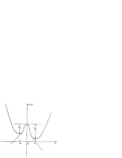
Figure 1: The general bistable potential in one dimension.

We now turn our attention to the bistable potential shown in Fig.(1). At $t=0$, we choose a probability distribution centered sharply around $x=0$, which is clearly a non-equilibrium function. Because of the inverted oscillator potential near the center, the distribution will broaden out in the initial stages. Thereafter, in an intermidiate time zone called the Suzuki regime, the broadened central peak begins to split into two side peaks corresponding to the minima of $U(x)$ at $x=a$ and $x=b$. Finally the system enters the Kramers’(1940) regime where it is close to equilibrium but makes occasional large fluctuation due to the noise. This Kramers regime will be governed by the lowest eigenvalue $\lambda_{1}$ of the system. The inverse of $\lambda_{1}$ sets the time scale for attaining equilibrium. The eigenvalue $\lambda_{1}$ is exponentially close to the ground state value $\lambda_{0}=0$ and differs from it due to the tunneling in the three-well problem. A WKB calculation of the eigenvalue was carried out by Caroli $\it{et}$ $\it{al.}$ (1979).

Here we will show a variational calculation (Bhattacharjee and Banerjee, 1989) motivated by the pioneering work of Bernstein and Brown (1984). The observation of Bernstein and Brown was that the Hamiltonian $H=\epsilon A^{{\dagger}}A$ and $\overline{H}=\epsilon AA^{{\dagger}}$ are surpersymmetric partners having the same spectrum except for the ground state. While the ground state energy of $H$ is zero, the same can not be true for $\overline{H}$ because the wave function satisfying $A^{{\dagger}}\phi=0$ cannot be normalized. The ground state of $\epsilon AA^{{\dagger}}$ is then the first excited state of $\epsilon A^{{\dagger}}A$. This is easily seen if we construct the matrix

$$H_{s}=\left(\begin{array}[]{c}\begin{array}[]{cc}\epsilon A^{{\dagger}}A&0\\ 0&\epsilon AA^{{\dagger}}\end{array}\end{array}\right)$$ (13)

The operator $Q$ with the representation $\left(\begin{array}[]{c}\begin{array}[]{cc}0&0\\ A&0\end{array}\end{array}\right)$ commutes with $H_{s}$ and hence $H_{s}$ has a degenerate spectrum. If $\psi$ is an eigenfuntion of $H_{s}$ with eigenvalue $\lambda$, then so is $Q\psi$. By inspection, one set of eigenvalues of $H_{s}$ can be written as $\psi_{n}=\left(\begin{array}[]{c}\phi_{n}\\ 0\end{array}\right)$ since (see Eqs.(8) and (9))

$$H_{s}\left(\begin{array}[]{c}\phi_{n}\\ 0\end{array}\right)=\epsilon\left(\begin{array}[]{c}A^{{\dagger}}A\phi_{n}\\ 0\end{array}\right)=\lambda_{n}\left(\begin{array}[]{c}\phi_{n}\\ 0\end{array}\right)$$ (14)

Consequently, we must have

$$H_{s}Q\left(\begin{array}[]{c}\phi_{n}\\ 0\end{array}\right)=H_{s}\left(\begin{array}[]{c}0\\ A\phi_{n}\end{array}\right)=\lambda_{n}\left(\begin{array}[]{c}0\\ A\phi_{n}\end{array}\right)$$ (15)

Since $\left(\begin{array}[]{c}0\\ A\phi_{n}\end{array}\right)=\left(\begin{array}[]{c}0\\ \epsilon AA^{{\dagger}}A\phi_{n}\end{array}\right)$, it follows that

$$\epsilon AA^{{\dagger}}A\phi_{n}=\lambda_{n}A\phi_{n}$$ (16)

Thus, $\lambda_{n}$ are the eigenvalues of $\epsilon AA^{{\dagger}}$ with eigenfunctions $A\phi_{n}$. This will be true for all $\phi_{n}$ except $\phi_{0}$. The eigenvalue zero is nondegenerate. For all other $\phi_{n}$ we have $\left(\begin{array}[]{c}0\\ A\phi_{n}\end{array}\right)$ and $\left(\begin{array}[]{c}\phi_{n}\\ 0\end{array}\right)$ as the degenerate eigenfunctions of $H_{s}$ and write $\phi_{n}$ are the eigenfunctions of $\epsilon A^{{\dagger}}A$; the $A\phi_{n}$ are the eigenfunctions of $\epsilon AA^{{\dagger}}$. To find the first excited state of $\epsilon A^{{\dagger}}A$ (the one corresponding eigenfunction $\phi_{1}$), we need to find the ground state of $\epsilon AA^{{\dagger}}$. Now that the problem is one of finding a ground state energy, this can be easily done by variational calculations.

We begin with the observation that the nonnormalizable wavefunction $\exp\Big{(}U(x)/2\epsilon\Big{)}$ satisfies $\epsilon AA^{{\dagger}}\exp\Big{(}U(x)/2\epsilon\Big{)}=0$. This motivates the choice of the wavefunction in the form $\exp\Big{(}\psi(x)/2\epsilon\Big{)}$ with

$$\psi(x)=\begin{cases}U(x),\qquad\qquad\qquad\text{for}\,\,b(1-\beta\epsilon^{1/2})\leq x\leq a(1-\alpha\epsilon^{1/2})\\ U(a-a\alpha\epsilon^{1/2})-U^{\prime}(a-a\alpha\epsilon^{1/2})(x-a+a\alpha\epsilon^{1/2}),\\ \,\,\,\qquad\qquad\qquad\qquad\text{for}\,x\geq a(1-\alpha\epsilon^{1/2})\\ U(a-a\beta\epsilon^{1/2})+U^{\prime}(a-a\beta\epsilon^{1/2})(x-b+\beta\epsilon^{1/2}),\\ \,\,\,\qquad\qquad\qquad\qquad\text{for}\,x\leq b(1-\beta\epsilon^{1/2})\end{cases}$$ (17)

In the above, we have assumed $\epsilon\ll 1$ and anticipated that the distance scale to be$\it{O}(\epsilon^{1/2})$, so that the variational parameters $\alpha$ and $\beta$ are numbers of $\it{O}(1)$. Note the matching occurs near the turning points in the classical regions for the corresponding Schrödinger equation. We need to evaluate

$$\lambda_{1}(\alpha,\beta)=\frac{\int^{\infty}_{-\infty}e^{\psi(x)/2\epsilon}[-\epsilon\frac{\partial^{2}}{\partial x^{2}}+\frac{U^{\prime}(x)^{2}}{4\epsilon}+\frac{U^{\prime\prime}(x)}{2}]e^{\psi(x)/2\epsilon}dx}{\int^{\infty}_{-\infty}e^{\psi(x)/\epsilon}dx}$$ (18)

The calculation involves the following steps :

(i) Evaluating the normalization integral. We note that $\psi(x)\simeq U(0)-\frac{1}{2}U^{\prime\prime}(0)x^{2}$ for $x<1$ and the maximum value of $\psi(x)$ dominates the integral for $\epsilon\ll 1$. Thus, the normalization integral is $e^{U_{0}/\epsilon}(2\pi\epsilon/U^{\prime\prime}(0))$.

(ii) The kinetic and potential energy term completely cancel $\psi(x)=U(x)$. Thus the integration in the numerator of Eq.(18) involves integrating from $a(1-\alpha\epsilon^{1/2})$ to $\infty$ and from $b(1-\beta\epsilon^{1/2})$ to $-\infty$.

(iii) In the range of integration discussed in (ii), it is sufficient to approximate the potential $U(x)$ by a quadratic expression for $\epsilon\ll 1$. Terms like $U(a-\alpha a\epsilon^{1/2})$ and $U^{\prime}(a-a\alpha\epsilon^{1/2})$ need to be expanded to $\it{O}(\epsilon)$, keeping in mind $U^{\prime}(a)=U^{\prime}(b)=0$. We thus obtain $\lambda_{1}(\alpha,\beta)$.

Minimizing $\lambda_{1}$ with respect to $\alpha$ and $\beta$ leads to the conditions:

$$a^{2}\alpha^{2}U^{\prime\prime}(a)=b^{2}\beta^{2}U^{\prime\prime}(b)=3$$ (19)

Thus, we find

$$\lambda_{1}=c[{\mid U^{\prime\prime}(0)\mid/U^{\prime\prime}(a)}^{1/2}e^{-\triangle_{a}/\epsilon}+{\mid U^{\prime\prime}(0)\mid/U^{\prime\prime}(b)}^{1/2}e^{-\triangle_{b}/\epsilon}]$$ (20)

with $\triangle_{a,b}=U(0)-U(a,b)$ and

$$c=\frac{1}{6}\frac{e^{3/2}}{(6\pi)^{1/2}}\simeq 0.17$$ (21)

For the WKB result of Caroli et al., $c=1/2\pi\simeq 0.159$.

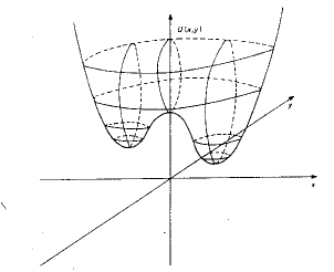
Figure 2: The general bistable potential in two dimensions.

To end this section, we consider generalization of the above treatment (Bhattacharjee and Banerjee, 1989) to higher dimensions. In two dimensions, the bistable potential $U(x,y)$ has the form shown in fig.(2). The important assumption about $U(x,y)$ is that there exists a most probable escape path (the instanton trajectory) connecting the two wells. In this case, we can always choose the axes such that the desired path is the x-axis. About this path, $U(x,y)$ can be expanded as

$$U(x,y)=U(x)+\frac{1}{2}W(x)y^{2}$$ (22)

In the above $U(x)$ is the one dimensional potential that we have already discussed. The Hamiltonian, corresponding to Eq.(5) can now be written as

$$H=-\epsilon\Bigg{(}\frac{\partial^{2}}{\partial x^{2}}+\frac{\partial^{2}}{\partial y^{2}}\Bigg{)}+V(x,y)$$ (23)

where

$$V(x,y)=\frac{1}{4\epsilon}\Bigg{[}\Bigg{(}\frac{\partial U}{\partial x}\Bigg{)}^{2}+\Bigg{(}\frac{\partial U}{\partial y}\Bigg{)}^{2}\Bigg{]}-\frac{1}{2}\Bigg{(}\frac{\partial^{2}U}{\partial x^{2}}+\frac{\partial^{2}U}{\partial y^{2}}\Bigg{)}$$ (24)

The ground state with zero eigenvalue is $\exp\Big{(}-U(x,y)/2\epsilon\Big{)}$. As before, our interest is in the first excited state.

We begin by noting that the first excited state will involve changes, mainly in the $x$-direction, retaining the $y$-dependence of the wavefunction as $\exp\Big{(}-W(x)y^{2}/2\epsilon\Big{)}$ to a good approximation. The ”stiffness” in the $y$-direction suggests a variant of the Born-Oppenheimer approximation. We solve the $y$-dependent part of the above Hamiltonian, treating the $x$-dependence as a parameter. The resulting eigenvalue will be a function of $x$ and can be treated as an effective potential for the one-dimentional problem in $x$. Introducing Eq.(22) into Eq.(23), the $y$-dependent Hamiltonian can be written as

$$H_{y}=-\epsilon\frac{\partial^{2}}{\partial y^{2}}+\frac{1}{4\epsilon}(W^{2}+U^{\prime}W^{\prime}-W^{\prime\prime}\epsilon)y^{2}$$ (25)

The lowest eigenvalue is $\frac{1}{2}(W^{2}+U^{\prime}W^{\prime}-\epsilon W^{\prime\prime})^{1/2}$ and we use this as an effective potential for the one dimensional problem in $x$. The function $W(x)$ is going to be slowly varying and we can expect $W^{\prime}/W$ and $W^{\prime\prime}/W$ to be small. This allows us a binomial expansion of the lowest eigenvalue and allows us to write the Hamiltonian as

$$H = -\epsilon\frac{d^{2}}{dx^{2}}+\frac{(U^{\prime})^{2}}{4\epsilon}-\frac{U^{\prime\prime}}{2}+\frac{U^{\prime}W^{\prime}}{4W}-\frac{\epsilon W^{\prime\prime}}{4W}$$

$$\simeq \epsilon\Bigg{[}-\frac{d}{dx}+\frac{U^{\prime}}{2\epsilon}+\frac{W^{\prime}}{4W}\Bigg{]}\Bigg{[}\frac{d}{dx}+\frac{U^{\prime}}{2\epsilon}+\frac{W^{\prime}}{4W}\Bigg{]}$$

where in the second step, we have deliberately not matched the higher-order term $(W^{\prime}/W)^{2}$. We require the two lowest eigenvalues of $H$ in Eq.(2). The lowest eigenvalue is of course known to be exactly zero and so it is the approximate determination of $\lambda_{1}$ which is our concern and that in accordance with our previous analysis, this is simply the ground state of the supersymmetric partner

$$\overline{H}=\epsilon\Bigg{[}\frac{d}{dx}+\frac{U^{\prime}}{2\epsilon}+\frac{W^{\prime}}{4W}\Bigg{]}\Bigg{[}-\frac{d}{dx}+\frac{U^{\prime}}{2\epsilon}+\frac{W^{\prime}}{4W}\Bigg{]}$$ (27)

We now take over the variational calculation for the one-dimensional case dicussed above. The only difference to be noted is that the non-normalizable function which gives zero eigenvalue is now

$$\psi(x)=\exp(U(x)/2\epsilon)\exp\Bigg{(}\frac{1}{4}\int^{x}_{0}\frac{W^{\prime}(x)}{W(x)}dx\Bigg{)}$$ (28)

For $\epsilon\ll 1$, the extra term yields the factor $\exp(\frac{1}{2}ln\frac{W(a)}{W(0)})$ for the range of integration $a(1-\alpha\epsilon^{1/2})$ to $\infty$ and a similar term for the range $b(1-\beta\epsilon^{1/2})$ to $-\infty$, when one calculates the expectation value. This leads to the answer

$$\lambda_{1}=c\Bigg{[}\Bigg{(}\frac{\mid U^{\prime\prime}_{0}\mid}{U^{\prime\prime}_{a}}\Bigg{)}^{1/2}(W_{a}/W_{0})^{1/2}e^{-\triangle_{a}/\epsilon}+\Bigg{(}\frac{\mid U^{\prime\prime}_{0}\mid}{U^{\prime\prime}_{b}}\Bigg{)}^{1/2}(W_{b}/W_{0})^{1/2}e^{-\triangle_{b}/\epsilon}\Bigg{]}$$ (29)

where the constant $c$ is once again $\frac{e^{3/2}}{6}\frac{1}{(6\pi)^{1/2}}$.

To end this section we would like to point out a formal analogy (Schneider et al., 1985) between a quantum problem with potential $V(x)$ and the Langevin process. In Eq.(5), if we write $t=i\tau$, we get the Schrödinger equation ($\epsilon=\hbar/2m,\widetilde{V}=\hbar V$)

$$i\hbar\frac{\partial\phi}{\partial\tau}=\frac{-\hbar^{2}}{2m}\frac{\partial^{2}\phi}{\partial x^{2}}+\widetilde{V}(x)\phi$$ (30)

and the stationary states in the $\tau$-variable are characterized by the eigenvalues $\lambda_{n}$. In the path integral formulation of quantum mechanics, this equation corresponds to the measure

$$d\mu(x,t) \sim e^{i/\hbar\int d\tau\Big{[}(m/2)(\frac{\partial x}{\partial\tau})^{2}-\widetilde{V}(x)\Big{]}}{\mathcal{D}}[x(\tau)]$$

$$\sim e^{-\int\frac{dt}{2m\epsilon}\Big{[}\frac{M}{2}(\frac{dx}{dt})^{2}+V(x)\Big{]}}{\mathcal{D}}[x(t)]$$

Turning to the Fokker-Planck equation, note that if at $t=0$, $x=0$, then $P(x,t_{0})=\delta(x-x_{0})$ and this fixes the coffecients $a_{n}$ in Eq.(7) as $a_{n}=\exp(\lambda_{n}t_{0})\phi_{n}(x_{0})/\phi_{0}(x_{0})$ leading to

$$P(x,t)=\phi_{0}(x)\sum_{n}\frac{\phi_{n}(x_{0})}{\phi_{0}(x_{0})}e^{-\lambda_{n}(t-t_{0})}\phi_{n}(x)$$ (32)

with $x=x_{0}$ at $t=t_{0}$. The two-time correlation follows from

$$<x(t)x(t_{0})> = \int dx\int dx_{0}P(x,t\mid x_{0},t_{0})xx_{0}P_{eq.}(x_{0})$$

$$= \int dxdx_{0}xx_{0}\phi_{0}(x)\sum^{\infty}_{n=0}\frac{\phi_{n}(x_{0})}{\phi_{0}(x_{0})}e^{-\lambda_{n}(t-t_{0})}\phi_{n}(x)\phi^{2}_{0}(x_{0})$$

$$= \sum^{\infty}_{n=0}e^{-\lambda_{n}(t-t_{0})}\int dx_{0}\phi_{0}(x_{0})x_{0}\phi_{n}(x_{0})\int dx\phi_{0}(x)x\phi_{n}(x)$$

$$= \sum_{n}\mid<0\mid x\mid n>\mid^{2}e^{-\lambda_{n}(t-t_{0})}$$

For $t\gg t_{0}$, only the lowest eigenvalue will contribute and hence

$$<x(t)x(0)>\longrightarrow\mid<0\mid x\mid 0>\mid^{2}+\mid<0\mid x\mid 1>\mid^{2}e^{-\lambda_{1}t}$$ (34)

This particular correlation function, this explores the lowest eigenvalue of the quantum problem. Correlation of composite variables will explore other eigenvalues $\lambda_{n}$. We thus arrive at the following result: If the spectrum of a quantum mechanical problem with potential $\widetilde{V}(x)$ is to be computed, then it should be possible to do that by studying a Langevin process with potential $U(x)$, where $U(x)$ and $V(x)$ are related as in Eq.(6). Integration of the stochastic differential equation then allows one to compute correlation function $<x(t)x(0)>$ as

$$<x(t)x(0)>=\lim_{T\to\infty}\frac{1}{T}\int x(t^{\prime})x(t^{\prime}+t)dt^{\prime}$$ (35)

The important issue is to find $U(x)$ if $V(x)$ is given. If the ground state energy of $H=T+V$, where $T$ is the kinetic energy is $\lambda_{0}$ (this will not be zero in general), then $U$ has to be found from

$$\frac{1}{4\epsilon}U^{\prime}(x)^{2}-(1/2)U^{\prime\prime}=V(x)-\lambda_{0}$$ (36)

If $\phi_{0}$ is the ground state of $H$, then

$$U=-2\epsilon\ln\phi_{0}$$ (37)

3 Suzuki Regime

In the bistable situations described in the previous section, the intermediate time zone where the probability distribution acquires bimodal character is also particularly important. We consider the evolution of an initial probability distribution $P(x,t=0)$ in the bistable potential $V(x)=-\frac{x^{2}}{2}+\frac{x^{4}}{4}$. At $t=0$, we assume that the probability is calculated about $x=0$ in a manner which is almost like a delta function (a very narrow Gaussian in reality). As time evolves, the distribution is going to spread out and then develop two peaks. The spreading is the initial time regime, while the intermediate time regime, where the probability distribution acquires the two peaks is called the Suzuki regime because of the interesting scaling observed by Suzuki (1977) in this time-zone. If the probality distribution explores only the small-$x$ part of the available space, then in the initial time regime, we can approximate $V(x)$ as $\widetilde{V}(x)=-x^{2}/2$. Carrying out the transformation $P(x,t)=\phi(x,t)\exp(-\widetilde{V}/2\epsilon)$,we find

$$\frac{\partial\phi}{\partial t}=\epsilon\frac{\partial^{2}\phi}{\partial x^{2}}-\Big{(}\frac{x^{2}}{4\epsilon}+\frac{1}{2}\Big{)}\phi=H\phi$$ (38)

The eigenvalues of the operator $H$ are clearly $-(n+1)$ with the eigenfunction $\phi_{n}=N_{n}\exp(-x^{2}/\epsilon)H_{n}(x/2\epsilon)$, where $H_{n}(y)$ is the $n^{th}$ Hermite polynomial and $N_{n}$ is the normalization constant. We can immediately write

$$P(x,t)=\sum C_{n}e^{-(n+1)t}N_{n}e^{-x^{2}/\epsilon}H_{n}(x/2\epsilon)$$ (39)

The constants $C_{n}$ are fixed by the initial form of $P(x,t)$. If we take the idealized form of $P(x,t=0)=\delta(x)$, then it follows that

$$P(x,t) = \sum e^{-(n+1)t}N_{n}e^{-x^{2}/\epsilon}H_{n}(0)H_{n}(x/2\epsilon)$$

$$= \frac{1}{[2\pi\epsilon(e^{2t}-1)]^{1/2}}e^{-\frac{x^{2}}{2\epsilon(e^{2t}-1)}}$$

It is obvious that the probability distribution spreads out in time since the width of the distribution is given by $2\epsilon(e^{2t}-1)\simeq 2\epsilon e^{2t}$. This is the initial time-regime, where the distribution sees the potential as an unstable inverted oscillator. The validity of the result for times such that $\epsilon e^{2t}\ll 1$ (ie. the spread is not too big) or $t\ll t_{0}\sim ln(1/\epsilon)$.

We now consider $t\gg t_{0}$ but much less than the Kramer’s time. In this limit the system ’slides down’ the potential and does not encounter the diffusion term Fokker-Planck equation. We can now write

$$\frac{\partial P}{\partial t} = \frac{\partial}{\partial x}\Big{[}P(-x+x^{3})\Big{]}$$

$$= (-x+x^{3})\frac{\partial P}{\partial x}+(3x^{2}-1)P$$

Writing $e^{t}=t^{\prime}$, we have

$$t^{\prime}\frac{\partial P}{\partial t^{\prime}}=(-x+x^{3})\frac{\partial P}{\partial x}+(3x^{2}-1)P$$ (42)

From the method of characterisation, we can write down the solution as

$$P(x,t) = \frac{1}{x(1-x^{2})}G\Big{(}x^{2}/(t^{\prime})^{2}(1-x^{2})\Big{)}$$

$$= \frac{1}{x(1-x^{2})}G\Big{(}\frac{e^{-2t}x^{2}}{1-x^{2}}\Big{)}$$

where $G(z)$ is an arbitrary function. As always G has to be obtained from the initial condition and in this case that is provided by Eq.(3). The initial condition also entails $x\ll 1$ and comparing with Eq.(3), we can obtain

$$P(x,t)=\frac{1}{x(1-x^{2})}\frac{1}{[2\pi\epsilon(e^{2t}-1)]^{1/2}}\exp\Big{(}-x^{2}/2(1-x^{2})\epsilon(e^{2t}-1)\Big{)}$$ (44)

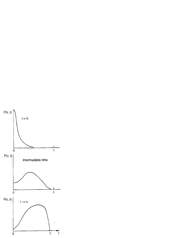
Figure 3: Time evolution of P(r,t)

What emerges is the new time scale $\tau=\epsilon e^{2t}$, which determines when the probality distribution will acquire the two peaked structure. [The sequence of $P(r,t)$ for the above function with $P(r,0)\simeq\delta(r)$ is shown in fig.(3).] We will demonstrate that the above answer is exact if consider a $N$-dimensional vector $x_{i}(t)$, $i=1,2,......,N$, with the stochastic time-evolution

$$\frac{\partial x_{\alpha}}{\partial t}=-\gamma\frac{\partial V}{\partial x_{\alpha}}+f_{\alpha}$$ (45)

with $V=-\frac{r^{2}}{2}+\frac{r^{4}}{4N}$ $r^{2}=\sum^{N}_{i=1}x_{i}^{2}$ and $f_{\alpha}$ is the random term with Gaussian correlation:

$$<f_{\alpha}(t_{2})f_{\beta}(t_{1})>=2\epsilon\delta(t_{1}-t_{2})$$ (46)

The fluctuation-dissipation relation holds with $\gamma=\epsilon$. The Fokker-Planck equation for $P({x_{\alpha}},t)$ is

$$\frac{\partial P}{\partial t}=\partial_{\alpha}\Big{(}P\frac{\partial V}{\partial x_{\alpha}}\Big{)}+\epsilon\frac{\partial^{2}P}{\partial x_{\alpha}\partial x_{\alpha}}$$ (47)

For the spherically symmetric $V$, we expect $P=P(r,t)$ and thus in spherical polar coordinate system, Eq.(47) reads

$$\frac{\partial P}{\partial t}=\epsilon\Big{(}\frac{\partial^{2}P}{\partial r^{2}}+\frac{N-1}{r}\frac{\partial P}{\partial r}\Big{)}+x_{\alpha}\Big{(}\frac{r^{2}}{N}-1\Big{)}\frac{\partial P}{\partial x_{\alpha}}+\Big{[}(1+2/N)r^{2}-N\Big{]}P$$ (48)

We define $R=N^{-1/2}r$ and get

$$\frac{\partial P}{\partial t}=\frac{\epsilon}{N}\frac{\partial^{2}P}{\partial R^{2}}+\frac{\epsilon(N-1)}{NR}\frac{\partial P}{\partial R}+R(R^{2}-1)\frac{\partial P}{\partial R}+[(N+2)R^{2}-N]P$$ (49)

In the limit $N\gg 1$ and $\epsilon\ll 1$, we drop the terms of $\it{O}(\epsilon)$, $\it{O}(N^{-1})$ and $\it{O}(\epsilon/N)$, to obtain

$$\frac{\partial P}{\partial t}+R(1-R^{2})\frac{\partial P}{\partial R}=[(N+2)R^{2}-N]P$$ (50)

The method of characteristics now yields

$$P(R,t)=\Big{(}\frac{1-R^{2}}{R^{2}}\Big{)}^{N/2}\Big{(}\frac{1}{1-R^{2}}\Big{)}^{1+N/2}G\Big{(}e^{2t}(1-R^{2})/R^{2}\Big{)}$$ (51)

Once again, this has to match smoothly to the small time solution in order to determine the unknown function $G$. Turning to Eq.(48), the short-time solution is given by

$$P(r\ll 1,t\ll t_{0}) = \Big{[}\frac{1}{2\pi\epsilon(e^{2t}-1)}\Big{]}^{N/2}e^{-\frac{r^{2}}{2\epsilon(e^{2t}-1)}}$$

$$= \Big{[}\frac{1}{2\pi\epsilon(e^{2t}-1)}\Big{]}^{N/2}e^{-\frac{NR^{2}}{2\epsilon(e^{2t}-1)}}$$

The matching is done by the choice

$$G\Big{(}e^{2t}(1-R^{2})/R^{2}\Big{)}=\Bigg{[}\frac{R^{2}}{1-R^{2}}\frac{N}{2\pi\epsilon(e^{2t}-1)}\Bigg{]}^{N/2}\exp\Bigg{[}-\frac{R^{2}}{1-R^{2}}\frac{N}{2\epsilon(e^{2t}-1)}\Bigg{]}$$ (53)

where $\exp(2t)$ has been replaced by $(\exp(2t)-1)$ since $\exp(2t)\gg 1$ and this replacement allows the matching with Eq.(3) to be implemented. This leads to the answer

$$P(R,t)=\Bigg{[}\frac{1}{2\pi\epsilon(e^{2t}-1)}\Bigg{]}^{N/2}\Bigg{(}\frac{1}{1-R^{2}}\Bigg{)}^{1+N/2}\exp\Bigg{[}-\frac{R^{2}}{1-R^{2}}\frac{N}{2\epsilon(e^{2t}-1)}\Bigg{]}$$ (54)

The discussion above is valid for a system of few degrees of freedom and as such the principle area of application is laser physics, where the laser operates as a pump parameter crosses a threshold value and then the exponential growth is checked by a cubic nonlinearity in the Langevin equation. The variable is the electric field which, for circularly polarised light, can be taken to be two-dimensional. The experimental measurements of the time-dependent intensity clearly shows the existence of Suzuki regime.

Of greater interest is the exploration of Suzuki scaling in the case of a field (Kawasaki et al., 1978; Bray, 1994), ie., a function of space and time, whose dynamics can be described by the Langevin equation

$$\frac{\partial\phi(\vec{r},t)}{\partial t}=-\frac{\delta F}{\delta\phi(\vec{r},t)}+f(\vec{r},t)$$ (55)

where $F$ is the ”free energy” which can be written as (in a $D$-dimensional space).

$$F=\int\Bigg{[}-\frac{a}{2}\phi^{2}+\frac{1}{2}({\bf{\nabla}}\phi)^{2}+\frac{1}{2}(\phi^{2})^{2}\Bigg{]}d^{D}x$$ (56)

In principle, $\phi$ may be a $N$-component vector, and $\phi^{2}=\sum_{i=1}^{N}\phi^{2}_{i}$ and $({\bf{\nabla}}\phi)^{2}=\sum_{i,j}(\partial_{i}\phi_{i})^{2}$.

The growth of order that we have been considering crresponds to the parameter $a$ being positive. if we work with the Fourier components $\phi(\vec{k},t)$ of $\phi(\vec{r},t)$, then

$$\frac{\partial\phi(\vec{k},t)}{\partial t}=(a-k^{2})\phi(\vec{k},t)-\lambda\sum_{\vec{k_{1}},\vec{k_{2}}}\phi(\vec{k_{1}},t)\phi(\vec{k_{2}},t)\phi(\vec{k}-\vec{k_{1}}-\vec{k_{2}},t)+f(\vec{k},t)$$ (57)

The probability distribution $P({\phi(k)},t)$ satisfies

$$\frac{\partial P(\phi(k),t)}{\partial t} = \sum_{k^{\prime}}\frac{\partial}{\partial\phi(k^{\prime})}\Bigg{[}P(-a+(k^{\prime})^{2})\phi(\vec{k^{\prime}},t)$$

$$+\lambda P\sum\phi(\vec{k_{1}},t)\phi(\vec{k_{2}},t)\phi(\vec{k^{\prime}}-\vec{k_{1}}-\vec{k_{2}},t)\Bigg{]}$$

$$+\sum_{k^{\prime}}\epsilon\frac{\partial^{2}P}{\partial\phi(k^{\prime})\partial\phi(-k^{\prime})}$$

The growth occurs for those $k$-values which are smaller than $a^{1/2}$, and our interest is in those wavenumbers alone. In the initial stages, where $\phi(x)$ is centred about $\phi=0$ and is small in magnitude, we can drop the cubic term in the above equation and the time-development will occur according to $P(\phi(k),t)\sim\prod\limits_{k^{\prime}}\exp\Bigg{(}-\mid\phi(k^{\prime})\mid^{2}/\epsilon e^{2rt}\Bigg{)}$, where $r=a-(k^{\prime})^{2}$. In the intermediate time-zone, it is the $\epsilon$-term in Eq.(3) that needs to be dropped and we need to find the solution for $P(\phi(k),t)$ as we did in Eq.(44). However, now it is more complicated.

Simplification occurs if we look at the derivation of Eq.(44) in slightly different manner. Returning to that case and setting $\epsilon=0$, implies in the Langevin picture solving the equation $\dot{X}=X-X^{3}$. The solution is $X(t)=Ce^{t}/(1+C^{2}e^{2t})^{1/2}$ where C is a constant. If we call $X_{0}(t)=Ce^{t}=X(0)e^{t}$, then clearly $X(t)=X_{0}(t)/[1+X^{2}_{0}(t)]^{1/2}$ and $X(0)=X(t)e^{-t}/[1-X^{2}(t)]^{1/2}$. We thus have a prescription for going to $X(0)$ from $X(t)$ and the evolution of $P(X,0)$ given as $e^{-X(0^{2})/\epsilon}$, will occur according to $P(X,t)\sim e^{-X^{2}/e^{2t}(1-X^{2})}$.

In the present case, this requires the solution of

$$\frac{\partial\phi(k)}{\partial t}=(a-k^{2})\phi(\vec{k})-\lambda\sum_{\vec{k_{1}},\vec{k_{2}}}\phi(\vec{k_{1}},t)\phi(\vec{k_{2}},t)\phi(\vec{k}-\vec{k_{1}}-\vec{k_{2}},t)$$ (59)

The solution $\phi(k)$ proceeds according to standard perturbative techniques. The simplification occurs in the large-time limit when we can identify a leading term at every order. This allows the summation of the perturbation series to yield

$$\phi(\vec{r},t)=\phi_{0}(\vec{r},t)/[1+\phi^{2}_{0}(\vec{r},t)]^{1/2}$$ (60)

with

$$\phi_{0}(\vec{r},t)=\exp(t(a+\nabla^{2}))\phi(\vec{r})$$ (61)

The inverse transformation is

$$\phi(\vec{r})=\exp(-t(a+\nabla^{2}))\phi(\vec{r})/[1-\phi^{2}(\vec{r})]^{1/2}$$ (62)

In the absence of the diffusion term the probability follows a Liouville equation which is a conservation law for the probability. Hence, if the initial distribution is known, then the distribution at any time can be obtained by the inverse transformation shown in Eq.(62).

The evolution of this probability distribution can be pictured as follows. In the initial period, fluctuations everywhere start growing rapidly and at the same time diffuse over the distance $(2rt)^{1/2}$, within which scale the fluctuations are strongly correlatad. Saturation sets in as the value of $\phi^{2}(\vec{r})$ at any point approaches unity. After a while, in the language of magnetism, the system breaks up into domains of size $(2rt)^{1/2}$ with the saturation magnetisation at$+1$ or $-1$.

Finally, we would like to point out connection with a field theory by writing the measure analogus to Eq.(2) as

$$d\mu\sim\exp(-S[\phi])\prod_{\alpha=1}{\mathcal{D}}\phi_{\alpha}(x,t)$$ (63)

where

$$S[\phi] = 1/\hbar\int^{\infty}_{-\infty}{\mathcal{H}}dt$$

$$= \int^{\infty}_{-\infty}dt\int d^{D}x\Big{[}\frac{\dot{\phi_{\alpha}}\dot{\phi_{\alpha}}}{4\epsilon}+V(\phi_{\alpha})\Big{]}$$

with the potential $V(\phi_{\alpha})$ coming from

$$V[\phi_{\alpha}]=\frac{1}{4\epsilon}\frac{\delta U}{\delta\phi_{\alpha}}\frac{\delta U}{\delta\phi_{\alpha}}-\frac{1}{2}\frac{\delta^{2}U}{\delta\phi_{\alpha}\delta\phi_{\alpha}}$$ (65)

With $t=i\tau$, the action is that for a quantum field theory with the action $S_{q}$, where

$$S_{q}=\int d\tau d^{D}x\Bigg{[}-\frac{1}{4\epsilon}\frac{d\phi_{\alpha}}{d\tau}\frac{d\phi_{\alpha}}{d\tau}+V(\phi_{\alpha})\Bigg{]}$$ (66)

If $U=(1/2)m^{2}\phi_{\alpha}\phi_{\alpha}+(1/2)({\bf{\nabla\phi_{\alpha}}})^{2}$, ie., the Langevin potential is quadretic, Eq.(65), prescribes

$$V[\phi_{\alpha}]=\frac{1}{4\epsilon}\Bigg{[}m^{4}\phi_{\alpha}\phi_{\alpha}-\frac{m^{2}}{2}-2m^{2}\phi_{\alpha}\frac{\partial}{\partial x_{\beta}}\frac{\partial\phi_{\alpha}}{\partial x_{\beta}}+\Bigg{(}\frac{\partial^{2}\phi}{\partial x_{\beta}\partial x_{\beta}}\Bigg{)}^{2}\Bigg{]}$$ (67)

Apart from constants,

$$S_{q}=\int d\tau d^{D}x\Bigg{[}-\frac{1}{4\epsilon}\frac{d\phi_{\alpha}}{d\tau}\frac{d\phi_{\alpha}}{d\tau}+\frac{m^{2}}{2\epsilon}\frac{\partial\phi_{\alpha}}{\partial x_{\beta}}\frac{\partial\phi_{\alpha}}{\partial x_{\beta}}+\frac{m^{4}}{4\epsilon}\phi_{\alpha}\phi_{\alpha}+\Bigg{(}\frac{\partial^{2}\phi}{\partial x_{\beta}\partial x_{\beta}}\Bigg{)}^{2}\Bigg{]}$$ (68)

which is a quadratic action and can be easily handled.

It is when $U$ is non trivial that one can generate non trivial $S_{q}$ and what would be interesting is to consider a nontrivial $S_{q}$(e.g., the one corresponding to the decay of the false vacuum (Coleman,1977)) and see if the corresponding Langevin dynamics can shed light on the quantum problem.

4 A Class of Time-Dependent Potentials

In this section, we will deal with potentials which are time-dependent but allow for the establishment of a final equilibrium state. This will be defferent from the time-dependences which are generally studied and have led to a wealth of interesting phenomena. These include the cases of diffusion over a barrier in the presence of harmonic force and diffusion over a fluctuating barrier. The hallmark of the former situation is the phenomenon of stochastic resonance (Benzi et al., 1981; Büttiker and Landauer, 1982; McNamara et al., 1988), where the signal-to-noise ratio of the response to an applied force displays a local maximum as a function of frequency. In the case of fluctuating barriers (Doering and Gadoua, 1992; Maddox, 1992; Zürcher and Doering, 1993; Pechukas and Hänggi, 1994), the discovery that the mean first passage time has a minimum as a function of the correlation time characterising the fluctuation has prompted a wide variety of investigations. What we would like to present here is a toy model for yet another kind of phenomenon-the global optimisation principle (Doye et al., 1999; Hunjan and Ramaswamy, 2002) on an evolving potential energy landscape. In such problems one is interested in finding the minima of a multidimensional potential energy surface which constitutes the energy landscape in problems such as protein folding or the finding the ground state configuration of atomic or molecular clusters. An interesting observation in this context is that of Hunjan et al.(to be published), who have shown that a continuously and adiabatically varying potential assists approach to desired configuration at $t\rightarrow\infty$ by avoiding trapping in local minima.

We want the final $(t=\infty)$ potential to be $V_{2}(x)$. We start from a different function and consider the time-dependent potential

$$V(x,t)=V_{2}(x)+b[V_{1}(x)-V_{2}(x)]\exp(-\lambda t)$$ (69)

which has the form $b[V_{1}(x)-V_{2}(x)]$ at $t=0$ and evolves to $V_{2}(x)$ at $t=\infty$. For $b=1$, $V_{1}(x)$ is the initial shape which evolves to $V_{2}(x)$. Our goal is to study the approach to equilibrium in such a system. It is clear that as $t\rightarrow\infty$ and $V\rightarrow V_{2}$, there is an equilibrium probability distribution $P_{eq}=\exp(-V_{2}/\epsilon)$ at $t=\infty$ for the Fokker-Planck equation.

To study the onset of equilibrium when V is of the form shown in Eq.(69), we make the usual substitution

$$P(x,t) = \phi(x,t)e^{-V(x,t)/2\epsilon}$$

$$= \phi(x,t)e^{-V_{2}(x)/2\epsilon}e^{-b\triangle Ve^{-\lambda t}/2\epsilon}$$

where

$$\triangle V=V_{1}(x)-V_{2}(x)$$ (71)

leading to

$$\frac{\partial\phi}{\partial t}=H_{0}\phi+H_{1}(t)\phi$$ (72)

with

$$H_{0}\phi=\epsilon\frac{\partial^{2}\phi}{\partial x^{2}}+\frac{1}{2}V^{\prime\prime}_{2}\phi-\frac{1}{4\epsilon}(V^{\prime}_{2})^{2}\phi$$ (73)

and

$$H_{1}=b\Bigg{[}\frac{\triangle V^{\prime\prime}}{2}-\frac{\lambda}{2\epsilon}\triangle V-\frac{V^{\prime}_{2}(\triangle V)^{\prime}}{2\epsilon}\Bigg{]}e^{-\lambda t}-b^{2}\frac{(\triangle V^{\prime})^{2}}{4\epsilon}e^{-2\lambda t}$$ (74)

In the above equation prime denotes differentiation with respect to $x$. The eigenvalues of $H_{0}$ are non-positive and we can write

$$H_{0}\psi_{n}=-E_{n}\psi_{n},\ with\ E_{n}\geq 0$$ (75)

The ground state $\psi_{0}$ has a space-independent part $V_{0}(t)$. We will separate out this part and write the general solution of Eq.(72) as

$$\phi(x,t)=\sum c_{n}(t)e^{-E_{n}t+\int^{t}V_{0}(t^{\prime})dt^{\prime}}\psi_{n}$$ (76)

The usual techniques of Dirac’s time dependent perturbation theory lead to

$$\dot{c_{n}}(t)=\sum_{m}c_{m}(t)<m\mid H_{2}\mid n>\exp[-(E_{m}-E_{n})t]$$ (77)

where $H_{2}=H_{1}-V_{0}$. Perturbation theory proceeds by expanding

$$c_{n}(t)=c_{n0}(t)+bc_{n1}(t)+b^{2}c_{n1}(t)+............$$ (78)

Introducing it in Eq.(77) yields

$$\dot{c_{n0}}=0$$ (79)

$$\dot{c_{n1}}(t)=\sum_{m}c_{m0}(t)<m\mid H\mid n>\exp[-(E_{m}-E_{n})t]$$ (80)

$$\dot{c_{n2}}(t)=\sum_{m}c_{m1}(t)<m\mid H\mid n>\exp[-(E_{m}-E_{n})t]$$ (81)

and so on. We see immediately that $c_{n0}=constant$, independent of time. Consequently, they are determined by the state of the system at $t=0$.

We focus on the where the final and initial potentials have qualitatively different structures. Our $V_{2}$ will be a double well potential, while our $V_{1}$ is the usual single well potential. Approach to equilibrium in the double well potential is strongly delayed, as we have seen in sec. 2, by the Kramers’ time which is a long time scale coming from the possibility of noise induced hopping from one minimum to another. Thus $V_{2}(x)=-\frac{x^{2}}{2}+\frac{x^{4}}{4}$, while $V_{1}(x)=x^{2}$.With this choice

$$H_{0}\phi=-\epsilon\phi^{\prime\prime}+\Bigg{(}\frac{(V^{\prime}_{2})^{2}}{4\epsilon}-\frac{V^{\prime\prime}_{2}}{2}\Bigg{)}\phi$$ (82)

$$H^{\prime} = \frac{3}{2}(1-x^{2})-(1/4\epsilon)x^{2}(3-x^{2})(1+x^{2})$$

$$- (\lambda/8\epsilon)x^{2}(6-x^{2})+(1/4\epsilon)x^{2}(3-x^{2})^{2}(1-e^{\lambda t})$$

The eigenvalues spectrum of $H_{0}$ is characterized, as we have seen before, by a set of close doublets as its low lying states. The separation within the doublet is exponentially small, while that between two doublets is of $\it{O}(1)$. The ground state is $E_{0}=0$ and the first exited state is the ground state of the supersymmetric partner of $\frac{(V^{\prime}_{2})^{2}}{4\epsilon}-\frac{V^{\prime\prime}_{2}}{2}$ and is exponentially small. The second exited state has an eigenvalue close to 2 and hence we can safely approximate the dynamics of the low lying states as that of a 2-atate system. If $\phi_{0}$ and $\phi_{1}$ are the two states and $0$ and $\delta$ the eigenvalues, then we can write

$$\phi(x,t)=c_{0}(t)\phi_{0}(x)+c_{1}(t)\phi_{1}(x)\exp(-\delta t)$$ (84)

Note that $\delta^{-1}$ is the Kramers’ time in the problem. The dynamics of $c_{0}$ and $c_{1}$ is governed by

$$\dot{c_{0}}=<\phi_{0}\mid H^{\prime}\mid\phi_{0}>e^{-\lambda t}c_{0}(t)+<\phi_{0}\mid H^{\prime}\mid\phi_{1}>c_{1}(t)e^{-\delta t}e^{-\lambda t}$$ (85)

$$\dot{c_{1}}=c_{0}<\phi_{1}\mid H^{\prime}\mid\phi_{0}>e^{\delta t}e^{-\lambda t}+c_{1}<\phi_{1}\mid H^{\prime}\mid\phi_{1}>e^{-\lambda t}$$ (86)

Now $H^{\prime}$ is even and hence $<\phi_{1}\mid H^{\prime}\mid\phi_{0}>=0$, which decouples $c_{0}$ and $c_{1}$ and we can easily integrate the above equations. If we drop terms like $\exp(-2\lambda t)$, we get

$$\dot{c_{1}}=c_{1}<\phi_{1}\mid\widetilde{H}^{\prime}\mid\phi_{1}>\exp(-\lambda t)$$ (87)

where

$$\widetilde{H}^{\prime}=(3/2)(1-x^{2})+(2x^{2}/4\epsilon)(3-x^{2})(1-x^{2})-(\lambda/8\epsilon)x^{2}(6-x^{2})$$ (88)

The dominant contributions to both $<\phi_{1}\mid\widetilde{H}^{\prime}\mid\phi_{1}>$ and $<\phi_{0}\mid\widetilde{H}^{\prime}\mid\phi_{0}>$ comes from near $x\simeq 1$. The small difference between the two matrix elements comes from the term $(3/2)(1-x^{2})$ in $H^{\prime}$, which is maximum near $x=0$ and at that point $\phi_{0}\not\simeq 0$ but $\phi_{1}\simeq 0$. After a set of straightforward manipulations, we see that

$$P(x,t)=P_{eq}(x)[1+f(x)\exp(-\delta_{eff}t)]$$ (89)

where

$$\delta_{eff}=\delta+\frac{3(1-e^{\lambda t})}{2\lambda t}\alpha$$ (90)

where $\alpha$ is a small number of the prder of $\delta$.

The approach to equilibrium is now through a modified Kramers’ time which is obtained from $\delta^{-1}_{eff}$. Clearly $\delta_{eff}>\delta$ and hence the new equilibration time is going to be smaller. Thus, in the toy model, we see a faster approach to equilibrium , which was the desired goal.

References

• [1] Benzi, R., Sutera, A. and Vulpiani, A. (1981). The mechanism of stochastic resonance. J. Phys. A, 14, L453.
• [2] Bernstein, M. and Brown, L.S. (1984). Supersymmetry and the Bistable Fokker-Planck equation. Phys. Rev. Lett., 52, 1933.
• [3] Bhattacharjee, J.K. and Banerjee, K. (1989). Kramers time in bistable potentials. J. Phys. A, 22, L1141.
• [4] Bray, A.J. (1994). Theory of phase ordering kinetics. Adv. Phys., 43, 357.
• [5] Buttiker, M. and Landauer, R. (1982). Traversal time for tunneling. Phys. Rev. Lett., 49, 1739.
• [6] Caroli, B., Caroli, C. and Roulet, B. (1979). Diffusion in a bistable potential: a systematic WKB treatment J. Stat. Phys., 21, 415.
• [7] Coleman, S. (1977). Fate of the false vacuum: semiclassical theory. Phys. Rev. D, 15, 2929.
• [8] Doering, C.R. and Gadoua, J.C. (1992). Resonant activation over a fluctuating barrier. Phys. Rev. Lett., 69, 2318.
• [9] Doye, J.P.K., Miller, M.A. and Wales, D.J. (1999). The double-funnel energy landscape of the 38-atom Lennard-Jones cluster. J. Chem. Phys., 110, 6896. See also Deaven, D.M. and Ho, K.M. (1995). Molecular geometry optimization with a genetic algorithm. Phys. Rev. Lett., 75, 288.
• [10] Hunjan J.S. and Ramaswamy, R. (2002). Global optimization by adiabatic switching. Int. J. Mol. Sci., 3, 30.
• [11] Hunjan, J.S., Matharoo, G.S., Sarkar, S. and Ramaswamy, R. (to be published).
• [12] Kawasaki, K., Yalabik, M.C. and Gunton, J.D. (1978). Growth of fluctuations in quenched time-dependent Ginzburg-Landau model systems. Phys. Rev. A, 17, 455.
• [13] Kramers, H.A. (1940). Brownian motion in a field of force and the diffusion model of chemical reactions Physica, 7, 284.
• [14] Maddox, J. (1992). Nature, 359, 771.
• [15] McNamara, B., Wiesenfeld, K. and Roy, R. (1988). Observation of stochastic resonance in a ring laser Phys. Rev. Lett., 60, 2626.
• [16] Pechukas, P. and Hanggi, P. (1994). Rates of activated processes with fluctuating barriers. Phys. Rev. Lett., 73, 2772.
• [17] Risken, H. (1984). Fokker-Planck Equation. Springer-Verlag, Berlin.
• [18] Schneider, T., Zannetti, M. and Badii, R. (1985). Stochastic simulation of quantum systems and critical dynamics. Phys. Rev. B, 31, 2941.
• [19] Suzuki, M. (1977). Scaling theory of transient phenomena near the instability point. J. Stat. Phys., 16, 11.
• [20] Zurcher, U. and Doering, C.R. (1993). Thermally activated escape over fluctuating barriers. Phys. Rev. E., 47, 3862.