Experimental observations of density fluctuations in an elongated Bose gas:
ideal gas and quasi-condensate regimes

Abstract

We report in situ measurements of density fluctuations in a quasi one dimensional ⁸⁷Rb Bose gas at thermal equilibrium in an elongated harmonic trap. We observe an excess of fluctuations compared to the shot noise level expected for uncorrelated atoms. At low atomic density, the measured excess is in good agreement with the expected “bunching” for an ideal Bose gas. At high density, the measured fluctuations are strongly reduced compared to the ideal gas case. We attribute this reduction to repulsive inter-atomic interactions. The data are compared with a calculation for an interacting Bose gas in the quasi-condensate regime.

In a classical gas, the mean square fluctuation of the number of particles within a small volume is equal to the number of particles (we shall call this fluctuation “shot noise”). On the other hand, because of quantum effects, the fluctuations in a non-condensed Bose gas are larger than the shot noise contribution Landau . For photons, the well known Hanbury Brown-Twiss or “photon bunching” effect is an illustration of this phenomenon BunchingOptique . Analogous studies have been undertaken to measure correlations between bosonic atoms released from a trap after a time of flight Yasuda96 ; Helium ; Folling2005 ; Esslinger . However, bunching in the density distribution of trapped cold atoms at thermal equilibrium has not been yet directly observed.

Density fluctuations of a cold atomic sample can be measured by absorption imaging as proposed in Grondalski99 ; Altman2004 and recently shown in Folling2005 ; Greiner2005 . When using this method, one necessarily integrates the density distribution over one direction, and this integration can mask the bunching effect whose correlation length is of the order of the de Broglie wavelength. A one dimensional (1D) gas, i.e. a gas in an anisotropic confining potential with a temperature lower than or of order of the zero point energy in two directions, allows one to avoid this integration, and is thus a very favorable experimental geometry.

Additionally, atoms in 1D do not Bose condense Hohenberg:1967 . One can therefore achieve a high degree of quantum degeneracy without condensation, which enhances the bunching effect for an ideal gas. When one considers the effect of interactions between atoms, two additional regimes can appear: the Tonks-Girardeau regime and the quasi-condensate regime kheruntsyan:053615 . Starting from an ideal gas, as one increases density at fixed temperature $T$, the 1D interacting Bose gas passes smoothly to the quasi-condensate regime. The linear density scale for this crossover is given by $n_{T}=(m(k_{B}T)^{2}/\hbar^{2}g)^{1/3}$ where $g$ is the effective 1D coupling constant and $m$ the atomic mass Kheru2003 ; Quasibec_Castin . Density fluctuations are suppressed by a factor $(n/n_{T})^{3/2}$ compared to the ideal gas (see Eq. (4) below), although phase fluctuations remain Dettmer2002 ; richard:010405 ; Helleg2003 ; Hugbart2005 ; shvarchuck2002 . We emphasize that this crossover occurs in the dense, weakly interacting limit which is the opposite of the Tonks-Girardeau regime.

To measure the density fluctuations of a trapped Bose gas as a function of its density, we acquire a large number of images of different trapped samples under identical conditions. We have access to both the ideal Bose gas limit, in which we observe the expected excess fluctuations compared to shot-noise, as well as the quasi-condensate regime in which repulsive interactions suppress the density fluctuations.

Our measurements are conducted in a highly anisotropic magnetic trap created by an atom chip. We use three current carrying wires forming an H pattern reichel:2002 and an external uniform magnetic field to magnetically trap the ⁸⁷Rb atoms in the $|F=2,m_{F}=2\rangle$ state (see Fig. 1). Adjusting the currents in the wires and the external magnetic field, we can tune the longitudinal frequency between 7 and 20 Hz while keeping the transverse frequency $\omega_{\perp}/(2\pi)$ at a value close to 2.85 kHz. Using evaporative cooling, we obtain a cold sample at thermal equilibrium in the trap. Temperatures as low as 1.4 $\hbar\omega_{\perp}/k_{B}$ are accessible with an atom number of $5\times 10^{3}$. The atomic cloud has a typical length of 100 $\mu$m along the $z$ axis and a transverse radius of 300 nm.

As shown in Fig. 1, in situ absorption images are taken using a probe beam perpendicular to the $z$ axis and reflecting on the chip surface at $45^{\rm o}$. The light, resonant with the closed transition $|F=2\rangle\rightarrow|F^{\prime}=3\rangle$ of the D2 line is switched on for 150 $\mu$s with an intensity of one tenth of the saturation intensity. Two images are recorded with a CCD camera whose pixel size $\Delta\times\Delta$ in the object plane is $6.0\times 6.0$ $\mu$m². The first image is taken while the trapping field is still on. The second image is used for normalization and is taken in the absence of atoms 200 ms later. During the first image, the cloud expands radially to about 5 $\mu$m because of the heating due to photon scattering by the atoms. The size of the cloud’s image is even larger due to resolution of the optical system (about 10 $\mu$m) and because the cloud and its image in the mirror at the atom chip surface are not resolved. Five pixels along the transverse direction $x$ are needed to include 95% of the signal.

We denote by $N^{\rm ph}_{i}(x,z)$ the number of photons detected in the pixel at position $(x,z)$ for the image $i$ $(i=1,2)$. We need to convert this measurement into an atom number $N(z)$ detected between $z$ and $z+\Delta$. Normally, one simply computes an absorption per pixel $\ln(N^{\rm ph}_{2}/N^{\rm ph}_{1})$ and sums over $x$:

$$N(z)=\sum_{x}\,\ln[N^{\rm ph}_{2}(x,z)/N^{\rm ph}_{1}(x,z)]\times\Delta^{2}/\sigma_{e},$$ (1)

where $\sigma_{e}$ is the absorption cross-section of a single atom. When the sample is optically thick and the atomic density varies on a scale smaller than the optical resolution or the pixel size, Eq. (1) does not hold since the logarithm cannot be linearized. In that case, Eq. (1) underestimates the atom number and the error increases with optical thickness. Furthermore, in our geometry, optical rays cross the atomic cloud twice since the cloud image and its reflexion in the atom chip surface are not resolved.

We partially correct for these effects by using in Eq. (1) an effective cross section $\sigma_{e}$ determined as follows. We compare the measured atom number using the in situ procedure described above with the measured atom number after allowing the cloud to expand and to leave the vicinity of the chip surface. In this case, Eq. (1) is valid and the atomic cross-section $\sigma_{0}=3\lambda^{2}/(2\pi)$ well known. We then obtain for the effective cross-section $\sigma_{e}=0.8\,\sigma_{0}$. Although this effective cross section depends on the atomic density, we have checked that for total atom number between $2\times 10^{3}$ and $9\times 10^{3}$ the measured value varies by only 10%. Taking into account the uncertainty on the value of $\sigma_{0}$, we estimate the total error on the measured atom number $N(z)$ to be less than 20%.

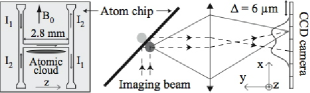
Figure 1: Schematic of the experimental setup. Left: drawing of the wires constituting the atom chip. We keep $I_{1}+I_{2}=3$ A and adjust $I_{1}-I_{2}$ between 0.3 A and 1 A to vary the confinement along $z$. The uniform field $B_{0}$ is approximately 40 G, we also add a small field ($\lesssim 1$ G) along $z$. Right: optical imaging system. We image the cloud and its reflection on the atom chip onto a CCD camera. In the radial direction, the unresolved cloud images cover approximately five pixels whose size in the object plane is $\Delta=6$ $\mu$m.

To measure the variance of the atom number in a pixel, we acquire a large number of images (typically 300) taken in the same experimental conditions. To remove technical noise from our measurement, the following procedure is used to extract the variance. For each image, we form the quantity $\delta N(z)^{2}=(N(z)-\bar{N}(z))^{2}$ where the mean value $\bar{N}(z)$ is normalized to contain the same total atom number as the current image. We thus correct for shot to shot total atom number fluctuations. The average is performed only over $p=21$ images which bracket the current image so that long term drifts of the experiment do not contribute to the variance. We have checked that the results are independent of $p$, varying $p$ between 5 and 21 . A large contribution to $\delta N(z)^{2}$, irrelevant to our study, is the photon shot noise of the absorption measurement. To precisely correct for this noise, we subtract the quantity $\sum_{x}(1/N^{\rm ph}_{1}(x,z)+1/N^{\rm ph}_{2}(x,z))(\Delta^{2}\sigma_{e})^{2}$ from $\delta N(z)^{2}$ for each image. We typically detect $10^{4}$ photons per pixel corresponding to a contribution to $\delta N^{2}$ of about 50. To convert the camera signal into a detected photon number, we use a gain for each pixel that we determine by measuring the photon shot noise of images without atoms as explained in jiang:521 . The corrected $\delta N(z)^{2}$ obtained for all images are then binned according to the value of $\bar{N}(z)$, rather than of $z$ itself. This gives the variance of the atom number $\langle\delta N(z)^{2}\rangle$ as a function of the mean atom number per pixel. Since more pixels have a small atom number, the statistical uncertainty on the estimate of the variance decreases with the average atom number (see Figs. (2) and (3)).

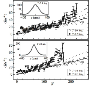
Figure 2: Atom number variance as a function of the mean atom number per pixel. Open circles correspond to a "hot" cloud ($k_{B}T\simeq 10\,\hbar\omega_{\perp}$, $\omega_{\perp}=2\pi\times 2.85$ kHz) for which fluctuations are given by the shot noise (black line). The full circles correspond to cold clouds. Error bars show the standard deviation of the mean of $\langle\delta N^{2}\rangle$. The fluctuations in excess of shot noise are due to bosonic bunching. The dot-dashed line is the prediction for an ideal Bose gas while the dotted line uses the Maxwell-Boltzmann approximation (see Eq. (3)). The insets show the longitudinal profile of the two cold clouds from which we deduce the temperature and the chemical potential used for the calculations.

Data shown in Fig. 2 correspond to atom clouds of sufficiently low density so that effect of inter-atomic interactions is expected to be small. The three data sets correspond to three different temperatures, the trapping frequencies are 2.85 kHz and 7.5 Hz. We deduce the temperature and the chemical potential of the sample by fitting the mean longitudinal profile $\bar{N}(z)$ of the cloud to the profile of an ideal Bose gas (see inset of Fig. 2). For the "hot" sample where bunching gives negligible contribution to $\delta N^{2}$ (see Eq. (3)), we observe atomic shot noise fluctuations, i.e. the atom number variance increases linearly with the mean atom number. The fact that we recover the linear behavior expected for shot noise increases our confidence in the procedure described in the previous two paragraphs. The slope $\kappa$ is only 0.17 and differs from the expected value of 1. We attribute this reduction to the fact that our pixel size is not much bigger than the resolution of our optical imaging system, thus one atom is spread out on more than one pixel. When the pixel size is small enough compared to the optical resolution and in the case of weak optical thickness, the expected slope is simply approximated by $\kappa\simeq\Delta/(2\sqrt{\pi}\,\delta)$ where $\delta$ is the rms width of the optical response which we suppose gaussian. From the measured slope, we deduce $\delta=10$ $\mu$m in good agreement with the smallest cloud image we have observed (8 $\mu$m).

For "cold" samples, we see an excess in the atom number variance compared to shot noise. We attribute this excess to bunching due to the bosonic nature of the atoms. In a local density approximation, the fluctuations of a radially trapped Bose gas with longitudinal density $n(z)$ are Glauber

$$\begin{array}[t]{l}\langle n(z)\,n(z^{\prime})\rangle-\langle n(z)\rangle^{2}=\langle n(z)\rangle\,\delta(z-z^{\prime})+\\ \displaystyle\frac{1}{\lambda_{\rm dB}^{2}}\sum_{i=1}^{\infty}\sum_{j=1}^{\infty}\frac{e^{\beta\mu(i+j)}}{\sqrt{ij}}\frac{e^{-\pi(z-z^{\prime})^{2}(\frac{1}{i}+\frac{1}{j})/\lambda_{\rm dB}^{2}}}{\left[1-e^{-\beta\hbar\omega_{\perp}(i+j)}\right]^{2}}\end{array}$$ (2)

where $\mu$ is the local chemical potential, $\beta=1/(k_{B}T)$, $\lambda_{\rm dB}=\sqrt{2\pi\hbar^{2}/(mk_{B}T)}$ is the de Broglie thermal wavelength and $\langle.\rangle$ denotes an ensemble average. The first term on the right hand side corresponds to shot noise, and the second term to bunching. For a non degenerate gas $(n\lambda_{\rm dB}\ll 1)$, one can keep only the term $i=j=1$. The bunching term reduces to $\langle n(z)\rangle^{2}\exp(-2\pi(z-z^{\prime})^{2}/\lambda_{\rm dB}^{2})\,\tanh^{2}(\beta\hbar\omega_{\perp}/2)$ and one recovers the well-known gaussian decay of the correlations. The reduction factor $\tanh^{2}(\beta\hbar\omega_{\perp}/2)$ is due to the integration over the transverse states. In our experiment, the pixel size is always much bigger than the correlation length. In which case, integrating over the pixel size $\Delta$, we have

$$\langle N^{2}\rangle-\langle N\rangle^{2}=\langle N\rangle+\langle N\rangle^{2}\frac{\lambda_{\rm dB}}{\sqrt{2}\Delta}\tanh^{2}(\beta\hbar\omega_{\perp}/2).$$ (3)

The coefficient of $\langle N\rangle^{2}$ is the inverse of the number of elementary phase space cells occupied by the $N$ atoms.

To compare Eq. (3) to our data we must correct for the optical resolution as was done for the shot noise. Furthermore, atoms diffuse about 5 $\mu$m during the imaging pulse because of photon scattering. This diffusion modifies the correlation function, but since the diffusion distance is smaller than the resolution, 10 $\mu$m, and since its effect is averaged over the duration of the pulse, its contribution is negligible. We thus simply multiply the computed atom number variance by the factor $\kappa$.

Figure 2 shows that the value calculated from Eq. (3) (dotted line) underestimates the observed atom number variance. In fact, for the coldest sample, we estimate $n(0)\lambda_{\rm dB}\simeq 10$, and thus the gas is highly degenerate. In this situation replacing the Bose-Einstein occupation numbers by their Maxwell-Boltzmann approximations is not valid, meaning that many terms of the sum in Eq. (2) have to be taken into account. The prediction from the entire sum is shown as a dot-dashed line and is in better agreement with the data.

In the experiment we are also able to access the quasi condensate regime in which inter-particle interactions are not negligible, and the ideal gas theory discussed above fails. Figure 3 shows the results of two experimental runs using denser clouds. For these data, the trapping frequencies are 2.85 kHz and 10.5 Hz. The insets show the mean longitudinal cloud profiles and a fit to the wings of the profiles to an ideal Bose gas profile. One can see from these insets that, unlike the conditions of Fig. 2, an ideal gas model does not describe the density profile in the center. We employ the same procedure to determine the variance versus the mean atom number. As in Fig. 2 we plot our experimental results along with the ideal Bose gas prediction based on the temperature determined from the fit to the wings in the insets. For small mean value $\bar{N}(z)$, the measured fluctuations follow the ideal gas curve (dot-dashed line) but they are dramatically reduced when the atom number is large.

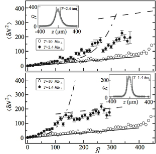
Figure 3: We plot the same quantities as in figure 2. Dot-dashed lines are the predictions for an ideal Bose gas (deduced from Eq. (2)), whereas the dashed lines show the results of Eq. (6). The temperature of the sample is deduced by fitting the wings of the longitudinal profile to an ideal Bose gas profile as shown in the insets. The solid lines gives the atomic shot noise level.

The theory for a weakly interacting uniform 1D Bose gas permits an analytical prediction for the density fluctuations in the limit $n\gg n_{T}$. In this limit, the gas enters the Gross-Pitaevskii regime and density fluctuations are given in the Bogoliubov approximation by Kheru2003 ; Quasibec_Castin

$$\begin{array}[t]{l}\langle\delta n(z)\,\delta n(z^{\prime})\rangle=\\ \displaystyle\frac{\langle n\rangle}{2\pi}\int_{-\infty}^{\infty}dk\,e^{ik(z-z^{\prime})}\left(\frac{k^{2}}{k^{2}+4\xi^{-2}}\right)^{1/2}(1+2n_{k}),\end{array}$$ (4)

where $n_{k}$ is the Bose thermal occupation factor of the mode $k$ with energy $\epsilon_{k}=\sqrt{k^{2}(k^{2}+4\xi^{-2})}\times\hbar^{2}/(2m)$ and $\xi=\hbar/\sqrt{mng}$ is the healing length. For 200 atoms per pixel, the healing length is about 0.3 $\mu$m in our experiment . The term proportional to $n_{k}$ describes the contribution of thermal fluctuations while the other is due to vacuum fluctuations. Since the pixel size is much bigger than the healing length, we probe only long wavelength fluctuations for which thermal fluctuations dominate at the temperatures we consider. Using $k\ll 1/\xi$ and $n_{k}\simeq k_{B}T/\epsilon_{k}$, we obtain for the atom number variance in a pixel

$$\langle N^{2}\rangle-\langle N\rangle^{2}=\Delta\frac{k_{B}T}{g}.$$ (5)

This formula can also be deduced from thermodynamic considerations: for a gas at thermal equilibrium, the atom number variance in a given volume is given by

$$\langle N^{2}\rangle-\langle N\rangle^{2}=k_{B}T(\partial N/\partial\mu)_{T}.$$ (6)

For a quasi-condensate with chemical potential $gn$, equations (5) and (6) coincide.

The calculation leading to Eq. (5) holds in a true 1D situation in which case the effective coupling constant is $g=2\hbar\omega_{\perp}a$, where $a$ is the scattering length of the atomic interaction. The validity condition for the 1D calculation is $n\ll 1/a$ (equivalently $\mu\ll\hbar\omega_{\perp}$). In our experiment however, the value of $na$ is as high as 0.7 and thus one cannot neglect dependence of the transverse profile on the local density. On the other hand, the thermodynamic approach is valid and, supposing $\mu(N)$ is known, Eq. (6) permits a very simple calculation. We use the approximate formula $\mu(N)=\hbar\omega_{\perp}\sqrt{1+4Na/\Delta}$ valid in the quasi-condensate regime gerbier:771 . This formula connects the purely 1D regime with that in which the transverse profile is Thomas-Fermi. The results of this analysis, confirmed by a full 3D Bogoliubov calculation, are plotted in Fig. 3 (dashed line). Equation (5) predicts a constant value for the atom number variance and underestimate it by 50% for the maximal density reached in our experiment ($\bar{N}=400$).

We compare this calculation in the quasi-condensate regime with our data. From Fig. 3 we see that the calculation agrees well with the measurements for $k_{B}T=1.4\,\hbar\omega_{\perp}$ but less so for $k_{B}T=2.4\,\hbar\omega_{\perp}$. The one-dimensional theory predicts that the quasi-condensate approximation is valid in the limit $n\gg n_{T}$ which corresponds to $\langle N\rangle\gg$ 100 (140) for $k_{B}T=1.4\,\hbar\omega_{\perp}$ ($k_{B}T=2.4\,\hbar\omega_{\perp}$). The disagreement between the calculation and our data for $k_{B}T=2.4\,\hbar\omega_{\perp}$ suggests that perhaps we did not achieve a high enough density to be fully in the quasi-condensate approximation. In addition the one-dimensional calculation of $n_{T}$ is unreliable for such high ratio $k_{B}T/\hbar\omega_{\perp}$ and underestimates the value at which the cross over appears. This is also the case for the data of Fig.2 where the naive estimate of $n_{T}$ corresponds to $\langle N\rangle=160$ for $k_{B}T=2.9\hbar\omega_{\perp}$ and $\langle N\rangle=130$ for $k_{B}T=2.1\hbar\omega_{\perp}$.

Exploitation of the 1D geometry to avoid averaging the fluctuations in the imaging direction can be applied to other situations. A Bose gas in the strong coupling regime, or an elongated Fermi gas should show sub shot noise fluctuations due to anti-bunching.

This work has been supported by the EU under grants IST-2001-38863, MRTN-CT-2003-505032, IP-CT-015714, by the DGA (03.34033) and by the French research ministry “AC nano” program. We thank D. Mailly from the LPN (Marcoussis, France) for helping us to micro-fabricate the chip.

References

- (1) L. Landau and E. Lifschitz, Statistical Physics, Part I, (Pergamon Press, Oxford, 1980), Chap. 12.
- (2) R. H. Brown and R. Q. Twiss, Nature 177, 27 (1956).
- (3) M. Yasuda and F. Shimizu, Phys. Rev. Lett. 77, 3090 (1996).
- (4) M. Schellekens et al., Science 310, 648 (2005).
- (5) S. Fölling et al., Nature 434, 481 (2005).
- (6) A. Öttl et al., Phys. Rev. Lett. 95, 090404 (2005).
- (7) J. Grondalski, P.M. Alsing and I. H. Deutsch, Optics Express 5, 249 (1999).
- (8) E. Altman, E. Demler, and M. D. Lukin, Phys. Rev. A 70, 013603 (2004).
- (9) M. Greiner et al., Phys. Rev. Lett. 94, 110401 (2005).
- (10) P. C. Hohenberg, Phys. Rev. 158, 383 (1967).
- (11) K. V. Kheruntsyan et al., Phys. Rev. A 71, 053615 (2005).
- (12) C. Mora and Y. Castin, Phys. Rev. A 67, 053615 (2003).
- (13) K. V. Kheruntsyan et al., Phys. Rev. Lett. 91, 040403 (2003).
- (14) S. Dettmer et al., Phys. Rev. Lett. 87, 160406 (2001).
- (15) S. Richard et al., Phys. Rev. Lett. 91, 010405 (2003).
- (16) D. Hellweg et al., Phys. Rev. Lett. 91, 010406 (2003).
- (17) M. Hugbart et al., Eur. Phys. J. D. 35, 155 (2005).
- (18) I. Shvarchuck et al., Phys. Rev. Lett. 89, 270404 (2002).
- (19) J. Reichel, Appl. Phys. B 74, 469 (2002).
- (20) Y. Jiang et al., Eur. Phys. J. D 22, 521 (2003).
- (21) M. Naraschewski and R. J. Glauber, Phys. Rev. A 59, 4595 (1999).
- (22) F. Gerbier, Europhys. Lett. 66, 771 (2004).