Suppression of quantum chaos in a quantum computer hardware

Abstract

We present numerical and analytical studies of a quantum computer proposed by the Yamamoto group in Phys. Rev. Lett. 89, 017901 (2002). The stable and quantum chaos regimes in the quantum computer hardware are identified as a function of magnetic field gradient and dipole-dipole couplings between qubits on a square lattice. It is shown that a strong magnetic field gradient leads to suppression of quantum chaos.

I Introduction

The fascinating idea of quantum computation stimulated numerous experimental efforts for realization of qubits based on various physical implementation of two-level quantum systems with controllable interactions (see e.g. Nielsen ). Liquid-state NMR implementation of quantum computation allowed to realize various quantum algorithms with few qubits including the Shor factoring algorithm Vandersypen1 and complex dynamics simulations corybaker . However, the liquid-state NMR scheme does not allow individual addressing of qubits and thus cannot lead to a large scale quantum computations schack . The situation can be significantly improved in the case of solid-state NMR implementation of quantum computation Nielsen . Certain features of this scheme appear also in the all-silicon quantum computer recently proposed by the Yamamoto group Yamamoto ; Ladd1 ; Ladd2 ; Ladd3 . In this proposal the qubits are spin-halves nuclei (e.g. isotopes ²⁹Si) placed on a 2D lattice on a surface of a crystalline solid matrix (e.g. of spin-0 ²⁸Si nuclei). A magnetic field gradient is assumed to be applied in the plane of the lattice to allow address qubits individually. At present large gradients can be realized experimentally Rugar ; Rugar1 and according to Yamamoto ; Ladd3 thousands of qubits can be addressed. In addition to qubit frequency gradient there are also dipole-dipole couplings between qubits typical of liquid-state NMR Slichter ; Vandersypen . These two elements, frequency gradient and dipole-dipole couplings between qubits, also appear in other proposals of quantum computers: e.g. for trapped polar molecules in electric field with gradient DeMille and trapped-ion spin molecules with magnetic gradient Twamley . Therefore the investigation of generic properties of such systems is important for future experimental implementations.

Indeed, it is known that the residual couplings between qubits lead to emergence of quantum chaos and melting of quantum computer hardware georgeot00 ; flambaum ; dls2001 . It has been also shown benenti ; frahm that these static imperfections give a rapid decrease of fidelity of quantum computations and hence their analysis is important to preserve high computation accuracy. For a 1D chain of qubits it has been shown that the introduction of frequency gradient generally makes the quantum hardware more stable against static inter-qubit couplings. This result may have important implications for proposals similar to those as in DeMille ; Twamley . However, a more generic 2D case proposed in Yamamoto still requires a special study. Such a detailed study is the main aim of this paper. To analyze the generic properties the quantum computer hardware Yamamoto we performed extensive numerical simulations with up to 18 qubits. Our studies show that a sufficiently strong field gradient leads to a suppression of quantum chaos and emergence of integrable regime where the real eigenstates become close to those of the ideal quantum computer without imperfections. On the basis of obtained results we determine the border between this integrable regime and quantum chaos region with ergodic eigenstates for various system parameters.

The structure of the paper is the following: in Section II we introduce typical physical parameters of the system, the results of numerical simulations and analytical estimates are presented in Section III and the discussion and conclusions are given in Section IV.

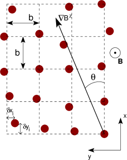
Figure 1: Disordered spin lattice: Local deviation from the vertex position $(n_{x_{i}}b,n_{y_{i}}b)$ is given by $\delta x_{i}=\delta_{x_{i}}b$ and $\delta y_{i}=\delta_{y_{i}}b$ (see text). The index $i$ labels the spins and runs from $1$ to $n_{q}=n_{x}n_{y}$. The magnetic field gradient has angle $\theta$ with $x$-axis (shown by arrow).

II Description of quantum computer model

Following the Yamamoto group proposal Yamamoto we introduce here a mathematical (YQC) model of a realistic quantum computer with field gradient and dipole-dipole couplings between qubits. For that we consider a two-dimensional array of $n_{q}$ nuclear spins 1/2 embedded in a crystalline solid, e.g. spin-1/2 ³¹P nuclei in a GaAs/AlGaAs quantum well or spin-1/2 ²⁹Si nuclei in a matrix of spin-0 ²⁸Si nuclei Yamamoto . In order to manipulate the nuclear spins using radio-frequency (RF) fields each qubit should be distinguishable, i.e. a specific Larmor frequency has to be assigned to each of them. The Hamiltonian of this array of nuclear spins is the following

$$\begin{array}[]{lcl}H&=&\sum_{i=1}^{n_{q}}\left(\omega_{0}+\delta\omega_{i}\right)I_{i}^{z}\\ &+&\sum_{i<j}d_{ij}\left(2I_{i}^{z}I_{j}^{z}-I_{i}^{x}I_{j}^{x}-I_{i}^{y}I_{j}^{y}\right).\end{array}$$ (1)

This Hamiltonian is widely used in NMR studies Slichter . The operators $I_{i}^{x,y,z}=\prod_{j=1}^{i-1}\mathbf{1}_{2}\otimes\frac{1}{2}\sigma^{x,y,z}\otimes\prod_{j=i+1}^{n_{q}}\mathbf{1}_{2}$ are the spin operators acting on the $i$th spin where $\sigma^{x,y,z}$ are the usual Pauli matrices. The frequency $\omega_{0}+\delta\omega_{i}$ is the Larmor frequency of the $i$th spin. Considering the spin-1/2 nuclei as an ensemble of qubits, $\omega_{0}+\delta\omega_{i}$ is the energy between the two states $\left\arrowvert\uparrow\right\rangle,\left\arrowvert\downarrow\right\rangle$ (or $\left\arrowvert 0\right\rangle,\left\arrowvert 1\right\rangle$) of a single qubit. The double sum runs over all the nuclei on the xy-plane and the term $d_{ij}=d/q^{3}_{ij}$ is the dipole coupling between the spins $i$ and $j$. Here $q_{ij}=r_{ij}/b$ is the distance between two spins $i$ and $j$ in units of the spin lattice constant $b$; $d$ is the coupling between two nearby spins on the square lattice ($q_{ij}=1$). In the Faraday geometry, i.e. the geometry where the magnetic field is orthogonal to the plane of the spin-1/2 nuclei ($\mathbf{B}=B^{z}\mathbf{\hat{z}}$), the coupling constant $d$ is given by $d=\mu_{0}\gamma^{2}\hbar^{2}/8\pi b^{3}$ where $\gamma$ is the gyromagnetic ratio of the considered nuclei. A schematic view of the structure is shown in Fig. 1. In the present work we keep focus on the regime $\omega_{0}\gg\delta\omega_{i},d$ where the single qubit energy $\omega_{0}$ is much bigger than the Larmor frequency shifts $\delta\omega_{i}$ and bigger than the dipole coupling $d_{ij}$ between the qubits. This corresponds to typical experimental conditions discussed in Yamamoto ; Ladd3 .

In (1) a particular Larmor frequency shift $\delta\omega_{i}$ is assigned to each nuclear spin. These Larmor frequency shifts are needed to distinguish one nuclear spin from the other, and can be seen as playing the same role as chemical shifts in liquid NMR Slichter . Here, these Larmor frequency shifts originate from a magnetic field gradient $\mathbf{g}=\bm{\nabla}B^{z}=g\mathbf{\hat{z}}$ lying on the xy-plane. For the $i$th nuclear spin located at the position $\mathbf{r}_{i}=n_{x_{i}}b\mathbf{\hat{x}}+n_{y_{i}}b\mathbf{\hat{y}}$ the Larmor frequency shift is

$$\delta\omega_{i}=\frac{\gamma}{2\pi}\mathbf{r}_{i}\cdot\bm{\nabla}B^{z}=n_{x_{i}}\omega_{g}\cos\theta+n_{y_{i}}\omega_{g}\sin\theta$$ (2)

where we define the characteristic frequency shift $\omega_{g}=\frac{\gamma}{2\pi}bg$. The Larmor frequency spacing between two nuclear adjacent spins along the $\hat{\mathbf{x}}$ (respectively the $\hat{\mathbf{y}}$) direction is $\omega_{gx}=\omega_{g}\cos\theta$ (respectively $\omega_{gy}=\omega_{g}\sin\theta$). In Tab. 1 typical physical parameters are given for the case of ³¹P and ²⁹Si nuclei. For example, if we consider a face-centered-cubic lattice of ³¹P nuclei with nearest neighbor distance $b=3.9974\mathrm{\AA}$ then $d=154\mathrm{Hz}$ and the regime $\omega_{g}/d=10$ in our simulations corresponds to $\omega_{g}=1540\mathrm{Hz}$ which is equivalent to a magnetic field gradient $g=0.224\mathrm{T/\mu m}$. If we consider now a lattice of ²⁹Si nuclei with nearest neighbor distance $b=1\mathrm{\AA}$ then $d=2.4\mathrm{kHz}$ and, for example, the regime $\omega_{g}/d=10$ in our simulations corresponds to $\omega_{g}=24\mathrm{kHz}$ which is equivalent to a magnetic field gradient $g=28\mathrm{T/\mu m}$.

	$|\gamma/2\pi|$	$b$	$d$	$\omega_{g}=10d$	$g\sim 10d/b$
31P	17.2 MHz/T	4 Å	154 Hz	1.54 kHz	0.224 T/$\mu$m
29Si	8.47 MHz/T	1.9 Å	346 Hz	3.46 kHz	2.15 T/$\mu$m
29Si	8.47 MHz/T	1 Å	2374 Hz	23.74 kHz	28.0 T/$\mu$m

Table 1: Typical physical parameters for different nuclei corresponding to $\omega_{g}/d=10$ in our simulations.

For a case of square lattice we consider the index $i$ labeling row by row each nucleus in the array and thus running from 1 to $n_{y}$ (first row) then from $n_{y}+1$ to $2n_{y}$ (second row) and this until $i=n_{q}=n_{x}n_{y}$. The angle $\theta$ for the direction of magnetic field gradient is measured in radians and due to symmetry we assume $\theta\leq\pi/4$. Experimentally, it is convenient to assign to the nuclei along the path indexed by $i$ the Larmor frequencies in ascending order. This ensures a total distinguishability of the nuclei. This condition is realized if $n_{y}\omega_{g}\sin\theta<\omega_{g}\cos\theta$. As the number of nuclei measured in a quantum dot can be as large as $n_{q}=n_{x}n_{y}\sim 10^{4}$, this condition becomes $\theta<n_{y}^{-1}$. Along the $\hat{\mathbf{x}}$ direction the Larmor frequency spacing between nearest neighbors is then $\omega_{gx}\simeq\omega_{g}\gg d$ and as a consequence the nuclei along that direction are highly distinguishable. The dipole coupling in (1) is then negligible. Along the $\hat{\mathbf{y}}$ direction the Larmor frequency spacing between nearest neighbors is $\omega_{gy}\simeq\omega_{g}/n_{y}\ll\omega_{g}$, the nuclei along that direction are weakly distinguishable. With $n_{y}\sim 10^{2}$ and using typical physical parameters of Tab. 1, we easily remark that along the $\hat{\mathbf{y}}$ direction the dipole couplings $d_{ij}$ cannot be neglected since $d\sim\omega_{gy}$.

In order to be more realistic we consider now the fact that the spins cannot form an ideal lattice, i.e. experimentally it is not possible to place each nucleus exactly on a regular rectangular lattice vertex. Consider the spin $i$ at the vicinity of the lattice vertex $(n_{x_{i}},n_{y_{i}})$. We define the deviations $\delta_{x_{i}}$ and $\delta_{y_{i}}$ which characterize the deviation of the spin $i$ from the ideal vertex position $(n_{x_{i}},n_{y_{i}})$. The position of the spin $i$ is then $\mathbf{r}_{i}=\left(n_{x_{i}}+\delta_{x_{i}}\right)b\mathbf{\hat{x}}+\left(n_{y_{i}}+\delta_{y_{i}}\right)b\mathbf{\hat{y}}$ (see Fig. 1). We assume that the deviations $\delta_{x_{i}}$ and $\delta_{y_{i}}$ are random and distributed in the interval $\left[-\delta/2,\delta/2\right]$ where $\delta$ is determined by an unavoidable experimental error in the nuclei positions. These spatial deviations modify weakly the dipole couplings $d_{ij}$ between nuclear spins as it depends on the inverse of the third power of the spin-spin distance $r_{ij}$. The main effect is the modification of the Larmor frequency shifts and as a consequence the Larmor frequency spacings between nuclear spins. For the $i$th spin the Larmor frequency shift is now

$$\delta\omega_{i}=\left(n_{x_{i}}+\delta_{x_{i}}\right)\omega_{gx}+\left(n_{y_{i}}+\delta_{y_{i}}\right)\omega_{gy}.$$ (3)

Thus the smallest Larmor frequency spacing between adjacent nuclear spins is

$$\begin{array}[]{lcl}\omega_{gx}^{\prime}&=&\min\left\{\delta\omega_{i+n_{y}}-\delta\omega_{i}\right\}_{i=1,n_{q}-n_{y}}\\ &=&\left(1-\delta\right)\omega_{gx}-\omega_{gy}\delta\end{array}$$ (4)

along the $\hat{\mathbf{x}}$ direction and

$$\begin{array}[]{lcl}\omega_{gy}^{\prime}&=&\min\left\{\delta\omega_{i+1}-\delta\omega_{i}\right\}_{i=1,n_{q}-1}\\ &=&\left(1-\delta\right)\omega_{gy}-\omega_{gx}\delta\end{array}$$ (5)

along the $\hat{\mathbf{y}}$ direction. For $\theta\in[0,\pi/4]$ and for $\delta<0.5$, $\omega_{gx}^{\prime}>0$ which ensures that along the path $i$ from one row to another the Larmor frequency increases. As we discussed before it is experimentally convenient that $\delta\omega_{i+1}-\delta\omega_{i}>0$ for each couple of adjacent Larmor frequency inside a row, i.e. along the $\hat{\mathbf{y}}$ direction. Using (5) this condition leads to the following inequality $\tan\theta>\delta/\left(1-\delta\right)$. Summarizing, for a large number $n_{y}$ of nuclei along the $\hat{\mathbf{y}}$ direction and small spatial imprecision $\delta\ll 1$ total distinguishability of the nuclei in the xy-plane will be achieved if the following condition is fulfilled

$$\delta<\theta<n_{y}^{-1}.$$ (6)

Note that the disorder introduced in (3) can also model the spatial inhomogeneity of the two-dimensional magnetic field gradient $\mathbf{g}$. Since the condition $\delta<n_{y}^{-1}$ has to be realized the condition of total distinguishability (6) imposes stringent experimental precision on the nuclei positions and on the two-dimensional magnetic field gradient.

In this paper we consider a typical experimental situation when the dipole couplings and the Larmor frequency shifts have comparable values $d\sim\omega_{g}$ but $\omega_{0}\gg\omega_{g},d$. In this regime, eigenstates of the Hamiltonian (1) can be ordered by spin sectors $\left\langle I^{z}\right\rangle=\left\langle\sum_{i}I_{i}^{z}\right\rangle$. Eigenstates with the same $\left\langle I^{z}\right\rangle$ value form an energy band of width $\delta\omega\simeq\omega_{g}\sqrt{n}_{q}$. Within this band $n_{\left\langle I^{z}\right\rangle}=n_{q}!/(n_{q}/2+\left\langle I^{z}\right\rangle)!(n_{q}/2-\left\langle I^{z}\right\rangle)!$ eigenstates are contained. Nearest bands, i.e. bands with a difference of $\pm 1$ in $\left\langle I^{z}\right\rangle$, are well separated in energy since their spacing is $\omega_{0}\gg\delta\omega$. In this case, using spin flip operators $I^{\pm}_{j}=I_{j}^{x}\pm iI_{j}^{y}$, the Hamiltonian (1) can be rewritten as

$$H=H_{\mathrm{diag}}+H_{\mathrm{off-diag}}$$ (7)

where

$$H_{\mathrm{diag}}=\sum_{i=1}^{n_{q}}\left(\omega_{0}+\delta\omega_{i}\right)I_{i}^{z}+2\sum_{i<j}d_{ij}I_{i}^{z}I_{j}^{z}.$$ (8)

is the diagonal part of the Hamiltonian and where

$$H_{\mathrm{off-diag}}=-\frac{1}{2}\sum_{i<j}d_{ij}\left(I_{i}^{+}I_{j}^{-}+I_{i}^{-}I_{j}^{+}\right)$$ (9)

is the off-diagonal part. From (8) we straightforwardly remark that the off-diagonal part of the Hamiltonian (7) is block diagonal, i.e. each block corresponds to a spin sector $\left\langle I^{z}\right\rangle$. This means that only noninteracting states with the same total spin value $\left\langle I^{z}\right\rangle$ are directly coupled by the dipole interaction. The diagonalization of any spin sector $\left\langle I^{z}\right\rangle$ can be performed independently of the others.

The Hamiltonian (7) determines the mathematical YQC model we study in this paper. Since the quantum chaos first appears in the middle of the spectrum georgeot00 , we study the properties of the Hamiltonian (1) in the central band which is associated to the $\left\langle I^{z}\right\rangle=0$ spin sector (respectively $\left\langle I^{z}\right\rangle=\pm 1/2$ spin sector) for even (respectively odd) number of spins. This part of the spectrum is most sensitive to imperfections and emergence of quantum chaos first starts here.

III Numerical results

In order to characterize the emergence of quantum chaos in the YQC model (7) we use the level spacing distribution $P(s)$ which clearly marks the transition from integrable to ergodic eigenstates (see e.g. Haake and Refs. therein). Here, $s=(\epsilon_{i+1}-\epsilon_{i})/\Delta$ is the normalized level spacing for energy levels $\epsilon_{i}$ in a close vicinity of the middle of the central band (we use 10% of the spectral bandwidth $\delta\omega$); $\Delta=\left\langle\epsilon_{i+1}-\epsilon_{i}\right\rangle$ is the mean level spacing in this vicinity. The form of $P(s)$ is linked to the ergodic properties of eigenstates: an integrable system has $P(s)$ in the form of the Poissonian distribution $P_{P}(s)=\exp(-s)$, and $P(s)$ is given by the Wigner-Dyson distribution of the random matrix theory $P_{WD}(s)=\left(\pi/2\right)s\exp(-\pi s^{2}/4)$ if the eigenstates are ergodic. Fig. 2 shows typical examples of the level spacing distribution $P(s)$ for a disorder strength $\delta=0.1$ and for a magnetic field gradient angle $\theta=0.3\mathrm{rad}$. Each distribution $P(s)$ in Fig. 2 have been calculated using 128700 energy levels and $N_{d}=10$ disorder configurations. As $\omega_{g}/d$ increases from $\omega_{g}/d=0$ to $\omega_{g}/d=10$ the distribution $P(s)$ changes from the Wigner-Dyson distribution to the Poissonian distribution. Thus the YQC hardware is in the regime of quantum chaos for $\omega_{g}<\omega_{g}^{c}$ while for $\omega_{g}>\omega_{g}^{c}$ it is in the integrable regime. According to the data of Fig. 2 the value of $\omega_{g}^{c}$ is located in the interval $4<\omega_{g}^{c}/d<7$.

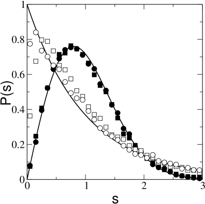
Figure 2: The level spacing distribution $P(s)$ for a case with disorder fluctuations amplitude $\delta=0.1$, for $\theta=0.3$, and for $\omega_{g}/d=1$ ($\bullet$), 4 ($\blacksquare$), 7 ($\square$), and 10 ($\circ$). The solid curves show the Poissonian and the Wigner-Dyson distributions. The number of disorder realizations is $N_{d}=10$. There are $n_{q}=16$ qubits placed on the lattice of size $4\times 4$.

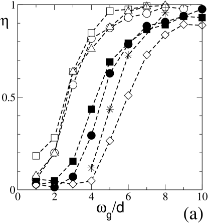
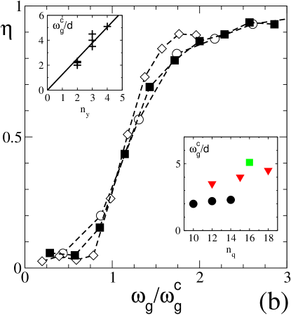
Figure 3: (a) Parameter $\eta$ as a function of $\omega_{g}/d$ for different lattice sizes $5\times 2$ ($\square$), $6\times 2$ ($\triangle$), $7\times 2$ ($\circ$), $4\times 3$ ($\blacksquare$), $5\times 3$ ($\bullet$), $6\times 3$ ($\ast$), and $4\times 4$ ($\diamond$). (b) Parameter $\eta$ as a function of the rescaled frequency shift $\omega_{g}/\omega_{g}^{c}$ where $\omega_{g}^{c}$ is defined by $\eta(\omega_{g}^{c}/d)=0.3$. For clarity only some curves presented in (a) are shown rescaled in (b). Upper inset: critical frequency shift $\omega_{g}^{c}$ as a function of $n_{y}$, the straight line shows the linear fit (see text). Lower inset: critical frequency shift as a function of the total number of qubits $n_{q}=n_{x}n_{y}$, where circles corresponds to $n_{y}=2$, triangles to $n_{y}=3$, and the square to $n_{y}=4$. In all cases $\delta=0.1$ and $\theta=0.3$. The number of disorder realization is $N_{d}=10$ ($N_{d}=4$ for the case $6\times 3$).

To investigate the quantum chaos border $\omega_{g}^{c}$ in more detail it is convenient to introduce the parameter Jacquod

$$\eta=\frac{\int_{0}^{s_{0}}\left[P(s)-P_{WD}(s)\right]ds}{\int_{0}^{s_{0}}\left[P_{P}(s)-P_{WD}(s)\right]ds}$$ (10)

where $s_{0}\simeq 0.4729$ is the first intersection point between the two distributions $P_{P}(s)$ and $P_{WD}(s)$. In this way $\eta$ tends to $0$ if the system is chaotic ($P(s)\rightarrow P_{WD}(s)$) and tends to $1$ if the system is integrable ($P(s)\rightarrow P_{P}(s)$). This parameter $\eta$ is rather convenient for investigation of the transition from integrability to quantum chaos and it has been used in various studies of many-body quantum systems georgeot00 ; Jacquod ; georgeotshard ; benentiepjd .

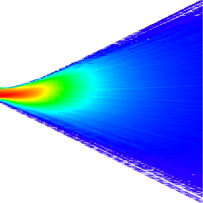
Figure 4: (Color online) Entropy $\mathcal{S}_{n}$ as a function of $\omega_{g}/d$, colors are proportional to the entropy. Red (gray) and blue (black) colors correspond to $\mathcal{S}_{n}\approx 13$ and $\mathcal{S}_{n}=0$ respectively; there are no eigenstates in the region with white color. Horizontal axis gives the value of $\omega_{g}/d$ from $\omega_{g}/d=0$ (left) to $\omega_{g}/d=20$ (right). Vertical axis gives the energies of the central band eigenstates (arbitrary units). The size of the lattice is $4\times 4$, $n_{q}=16$. Disorder corresponds to $\delta=0.1$ and $\theta=0.3$rad. All the points on the figure has been computed for the same realization of the disorder.

In Fig. 3 we show the dependence of $\eta$ on the frequency shift $\omega_{g}$ for different lattice sizes at a typical values of angle $\theta=0.3$ and disorder strength $\delta=0.1$. The transition from a regular regime ($\omega_{g}>\omega_{g}^{c}$) to a chaotic one ($\omega_{g}<\omega_{g}^{c}$) is clearly seen for each presented lattice size. In order to monitor the transition more precisely by the dependence of $\omega_{g}^{c}$ on parameters, we define $\omega_{g}^{c}$ by the condition $\eta(\omega_{g}^{c}/d)=0.3$. Fig. 3b shows $\eta$ as a function of the rescaled frequency shift $\omega_{g}/\omega_{g}^{c}$. The lower inset of Fig. 3b clearly shows that $\omega_{g}^{c}$ is not a single-valued function of $n_{q}$. This can be seen also in Fig. 3a where the lattice configurations $6\times 2$ and $4\times 3$ corresponding to the same number of qubits $n_{q}=12$ give two different curves of $\eta$ and thus give two different values of $\omega_{g}^{c}$. The upper inset of Fig. 3b shows that $\omega_{g}^{c}$ is satisfactory described by a linear dependence. A linear fit gives $\omega_{g}^{c}=1.26n_{y}d$. Also the main panel of Fig. 3b shows that the transition towards integrability becomes sharper as $n_{y}$ increases. Hence, for a $100\times 100$ array of ³¹P spin-1/2 with a nearest-neighbour ³¹P-³¹P distance $b=4\mathrm{\AA}$, a magnetic field gradient of at least $g_{c}=2.8$T$/\mu$m is needed in order to avoid emergence of quantum chaos in the static quantum computer hardware.

The dependence found numerically

$$\omega_{g}^{c}=Cdn_{y}$$ (11)

with a constant $C\approx 1.3$ can be understand on the basis of the Åberg criterion aberg . This criterion has been proposed aberg to understand the conditions of emergence of quantum chaos and ergodicity in many-body quantum systems. The extensive numerical tests combined with analytical estimates have been performed in sushkov ; Jacquod ; georgeot00 ; georgeotshard ; dls2001 ; benentiepjd ; Berman1 that allowed to establish the conditions of emergence of quantum chaos and dynamical thermatization in variety of many-body quantum systems. According to these results the quantum chaos emerges when the coupling strength $U$ becomes comparable to the spacing between directly coupled noninteracting states $\Delta_{c}$, i.e. when $U\sim\Delta_{c}$. It is important to stress that $\Delta_{c}$ is exponentially larger than the level spacing between many-body quantum states which for YQC is of the order of $\Delta_{n}\sim\omega_{g}n_{q}2^{-n_{q}}$.

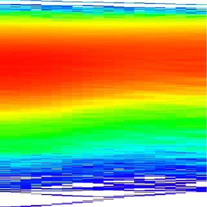
Figure 5: (Color online) Entropy $\mathcal{S}_{n}$ for $\omega_{g}/d=4$ as a function of the magnetic field gradient angle $\theta$. Colors are as in Fig. 4. Horizontal axis gives the value of $\theta$ from $\theta=0$ (left) to $\theta=\pi/4$ (right). Vertical axis gives the energies of the central band eigenstates (arbitrary units). Disorder strength is $\delta=0.1$. All the points on the figure has been computed for the same realization of the disorder as in Fig4 at the lattice size $4\times 4$.

In our model the noninteracting quantum register states are eigenstates $\left\arrowvert\phi_{i}\right\rangle$ of the diagonal Hamiltonian $H_{\mathrm{diag}}$ (9). The off-diagonal part $H_{\mathrm{off-diag}}$ (9) contains flip-flop operators and couples these noninteracting states thus being responsible for the emergence of quantum chaos in the system. The ensemble of the noninteracting states $\left\{\left\arrowvert\phi_{i}\right\rangle\right\}_{i=1,N_{H}}$ forms the quantum register basis, i.e., the basis is composed of $N_{H}=2^{n_{q}}$ states with $N_{H}$-dimensional vectors written in $\left(\left\arrowvert\uparrow\right\rangle,\left\arrowvert\downarrow\right\rangle\right)$ or $\left(\left\arrowvert 0\right\rangle,\left\arrowvert 1\right\rangle\right)$ representation (e.g. $\left\arrowvert\phi_{i}\right\rangle=\left\arrowvert 0010100111...01001\right\rangle$). The quantum register gives a convenient computational basis to perform quantum computations Nielsen , each multiqubit state is then a linear superposition of quantum register vectors $\left\arrowvert\phi_{i}\right\rangle$.

To apply the Åberg criterion to the YQC model we note that the dipole interactions $d_{ij}=d/q_{ij}$ vanish quickly with the interqubit distance and thus we can consider that only first (at most second) nearest neighbours qubits are coupled together. This means that $U\sim d$. For $\theta\ll 1$ the states coupled by transitions $H_{\mathrm{off-diag}}$ (9) have a typical energy change $\omega_{g}$ (assuming that only few rows in $x$ contributes) and the number of such transitions is of the order of $n_{y}$. Thus $\Delta_{c}\sim\omega_{g}/n_{y}$ that leads to the result (11). For $\theta\sim 1$ still the transitions in the direction perpendicular to the field gradient dominate so that in the relation (11) $n_{y}$ should be replaced by $\sqrt{n_{q}}$ that gives

$$\omega_{g}^{c}=Cd\sqrt{n_{q}}\;\;,(\theta\sim 1)$$ (12)

with $C\sim 1$.

Figure 6: Parameter $\eta$ as a function of the magnetic field gradient angle $\theta$ for $\omega_{g}/d=3$ ($\bullet$), 4 ($\blacksquare$), and 7 ($\blacktriangle$). The disorder strength is $\delta=0.1$. The lattice size is $5\times 3$, $N_{d}=10$.

The emergence of quantum chaos manifests itself not only in the level spacing statistics but also in the complexity of quantum eigenstates in presence of interactions. To demonstrate this fact in a quantitative way it is convenient to define the complexity of an eigenvector $\left\arrowvert\psi_{n}\right\rangle$ by its entropy $\mathcal{S}_{n}=-\sum_{i=1}^{N_{H}}w_{ni}\log_{2}w_{ni}$ where $w_{ni}=\left\arrowvert\left\langle\phi_{i}\arrowvert\psi_{n}\right\rangle\right\arrowvert^{2}$. Here $\left\{\left\arrowvert\phi_{i}\right\rangle\right\}_{i=1,N_{H}}$ is the quantum register basis, or computational basis composed of $N_{H}=2^{n_{q}}$ states. Here, $N_{H}$-dimensional vectors are written in the $\left(\left\arrowvert\uparrow\right\rangle,\left\arrowvert\downarrow\right\rangle\right)$ or $\left(\left\arrowvert 0\right\rangle,\left\arrowvert 1\right\rangle\right)$ representation (e.g. $\left\arrowvert\phi_{i}\right\rangle=\left\arrowvert 0010100111...01001\right\rangle$). The entropy $\mathcal{S}_{n}$ quantifies the deviation of the eigenvector $\left\arrowvert\psi_{n}\right\rangle$ from a pure quantum register state. If $\mathcal{S}_{n}=0$, $\left\arrowvert\psi_{n}\right\rangle=\left\arrowvert\phi_{n}\right\rangle$ is a quantum register state. If $\mathcal{S}_{n}=n_{q}$, all the quantum register states $\left\arrowvert\phi_{i}\right\rangle$ are equally present in the eigenvector $\left\arrowvert\psi_{n}\right\rangle$. As we particularly focus on the central band eigenstates, the maximum entropy attainable is $\mathcal{S}_{n}=-\log_{2}\binom{N}{\left[N/2\right]}<n_{q}$ for an eigenstate $\left\arrowvert\psi_{n}\right\rangle$ equally composed by all the quantum registers $\left\arrowvert\phi^{B}_{i}\right\rangle$ belonging to the $\left\langle I^{z}\right\rangle=0$ (even case) or $\pm 1$ (odd case) sector. Indeed the symmetry of the Hamiltonian (1) and the fact that $\omega_{0}\gg\omega_{g}>d$ guarantee that the central band eigenstates $\left\arrowvert\psi_{n}\right\rangle$ can only be linear superposition of the $\left\arrowvert\phi^{B}_{i}\right\rangle$ quantum registers.

Fig. 4 shows $\mathcal{S}_{n}$ as a function of $\omega_{g}/d$ for a disorder strength $\delta=0.1$ and a magnetic field gradient angle $\theta=0.3\mathrm{rad}$. It is clearly seen that the entropy of eigenstates is reduced significantly with the increase of magnetic field gradient. Thus a high gradient gives a suppression of quantum chaos in the YQC model. The dependence of entropy on the angle $\theta$ of magnetic field gradient is shown in Fig. 5. In agreement with the theoretical estimates (11), (12) there is no significant dependence on $\theta$. This is also true for the level spacing statistics as it is demonstrated in Fig. 6 where the parameter $\eta$ is clearly independent of $\theta$.

The dependence of $\eta$ on the disorder strength $\delta$ is presented in Fig. 7. At weak and moderate values of rescaled field gradient $\omega_{g}/d$ an increase of $\delta$ drives the system to a more integrable regime with higher values of $\eta$. This tendency is similar to those found in georgeot00 where disorder also stabilized the integrable phase. However, in the YQC model this effect is weaker. Indeed, the increase of $\delta$ gives an increase of $\Delta_{c}$ but not more than by a factor of two since there is always a contribution from a regular field gradient. It is interesting to note that according to the data of Fig. 7 in absence of disorder the system is completely in the regime of quantum chaos ($\eta\approx 0$) at a small field gradient ($\omega_{g}/d\leq 2$). This means that at $\omega_{g}/d\leq 2$ dipole-dipole interactions between qubits lead to a melting of quantum computer hardware and destruction of ideal computational basis.

Figure 7: Parameter $\eta$ as a function of the disorder strength parameter $\delta$ for $\omega_{g}/d=2$ ($\bullet$), 4 ($\blacksquare$), and 6 ($\blacktriangle$). The magnetic field gradient angle is $\theta=0.3\mathrm{rad}$. The lattice size is $5\times 3$, $N_{d}=10$.

Figure 8: Dependence of the width $\Gamma$ of the local density of states $\rho_{W}$ on the frequency shift $\omega_{g}$ for a disorder $\delta=0.1$ at a magnetic field gradient angle $\theta=0.3$rad and a number of qubit $n_{q}=n_{x}n_{y}=5\times 3$. The dashed line shows the gaussian regime with $\Gamma\propto d$ and the full line shows the Breit-Wigner regime with $\Gamma\propto d^{2}/\omega_{g}$. Lower inset: an example of the local density of states $\rho_{W}$ for $\omega_{g}/d=3$; the full curve shows the best fit of the Breit-Wigner form with $\Gamma=2.1d$. Upper inset: example of the local density of states $\rho_{W}$ for $\omega_{g}/d=1$; the full curve shows the best Gaussian fit of width $\Gamma=2.52d$. In both insets $\epsilon/d$ is rescaled energy, crosses give numerical data. The transition towards integrability takes place near $\log\left(\omega_{g}/d\right)\approx 0.7$ that corresponds to the quantum chaos border (11).

To determine the melting rate of the quantum computer hardware we compute numerically the local density of states $\rho_{W}$ (see e.g. georgeot00 ) defined as

$$\rho_{W}(E-E_{i})=\sum_{n}w_{ni}\delta(E-E_{n})$$ (13)

where $E_{i}$ is the energy of ideal quantum computational state $\phi_{i}$ given by $H_{\mathrm{diag}}$ (8). The energy width $\Gamma$ of this distribution gives the rate on emergence of quantum chaos georgeot00 ; flambaum . Thus in the regime of quantum chaos $\omega_{g}<\omega_{g}^{c}$ exponentially many states are mixed after a time scale $1/\Gamma$ (here $\hbar=1$). The number of mixed states is of the order of $\Gamma/\Delta_{n}$ where $\Delta_{n}$ is a typical level spacing between many-body states. For weak couplings between qubits the distribution $\rho_{W}(E)$ has the Breit-Wigner shape with the width $\Gamma\sim U^{2}/\Delta_{c}$ (see e.g. georgeot00 ; flambaum ). For the YQC case this gives

$$\Gamma\sim d^{2}\sqrt{n_{q}}/\omega_{g}\;.$$ (14)

For strong couplings $d$ (at $\Gamma>\Delta_{c}$) the width starts to grow linearly with coupling $\Gamma\sim d{n_{q}}^{1/4}$ similar to the case considered in georgeot00 ; flambaum ; flambaum1 . In this case $\rho_{W}(E)$ has a gaussian shape. The numerical data shown in Fig. 8 for 18 qubits confirm these theoretical formulas. Indeed, for small $\omega_{g}/d$ the width $\Gamma$ is independent of $\omega_{g}$ and $\rho_{W}(E)$ has a gaussian shape, while for larger $\omega_{g}/d$ the distribution $\rho_{W}(E)$ starts to have the Breit-Wigner shape and $\Gamma\propto 1/\omega_{g}$ in agreement with (14). For even larger values of $\omega_{g}/d$ one starts to enter in the integrable regime $\omega_{g}>\omega_{g}^{c}$ where the relation (14) is not valid anymore. The place of the transition is in a good agreement with the quantum chaos border (11) which gives $\omega_{g}^{c}=3.9d$ (to be compared with the approximate value $\omega_{g}^{c}\approx 5d$ obtained from data of Fig. 8).

Thus an extensive amount of numerical data obtained with up to 18 qubits give good agreement with the theoretical estimates derived for the YQC model.

IV Conclusion

The numerical and analytical studies presented above establish the parameter regime where the ideal computational basis of the quantum computer model (YQC) proposed in Yamamoto remains robust in respect to dipole-dipole couplings between qubits. They clearly show that a presence of magnetic field gradient allows to suppress quantum chaos in the quantum computer hardware if the gradient $g$ is larger than the quantum chaos border given by Eqs. (11), (12). For typical parameters of Table I (e.g. ²⁹Si, $b=1.9$Å) the YQC hardware is in the stable regime at $g\approx 2$ T/$\mu$m for $n_{q}=100$ qubits and at $g\approx 20T/\mu m$ for $n_{q}=10^{4}$ qubits. These values can be realized with modern experimental methods.

At the same time we should also note that the stability of a quantum computer hardware is not necessary sufficient for high accuracy of quantum computations. Indeed, here we analyzed only the static properties of YQC. In a realistic YQC implementation it is also necessary to consider the accuracy of gate implementations and the effects of static imperfections on the accuracy of a concrete operating quantum algorithm (see e.g. frahm ). Future investigations are required to analyze such operational accuracy of the YQC model Yamamoto .

We thank T.D.Ladd and Y.Yamamoto for discussions of the specific properties of the quantum computer proposed in Yamamoto . This work was supported in part by the EC IST-FET project EDIQIP.

References

- (1) M. A. Nielsen and I. L. Chuang, Quantum Computation and Quantum Information (Cambridge University Press 2000).
- (2) L. M. K. Vandersypen, M. Steffen, G. Breyta, C. S. Yannoni, M. H. Sherwood, and I. L. Chuang, Nature 414, 883 (2001).
- (3) Y.S. Weinstein, S.Lloyd, J.Emerson, and D.G. Cory, Phys. Rev. Lett. 89, 157902 (2002).
- (4) S.L.Braunstein, C.M.Caves, R.Jozsa, N.Linden, S.Popescu, and R. Schack, Phys. Rev. Lett. 83, 1054 (1999).
- (5) T. D. Ladd, J. R. Goldman, F. Yamaguchi, and Y. Yamamoto, Phys. Rev. Lett. 89, 017901 (2002).
- (6) F. Yamaguchi, T. D. Ladd, C. P. Master, Y. Yamamoto, and N. Khaneja, quant-ph/0411099.
- (7) K.-M. C. Fu, T. D. Ladd, C. Santori, and Y. Yamamoto, Phys. Rev. B 69, 125306 (2004).
- (8) J.R. Goldman, T.D. Ladd, F. Yamaguchi, and Y. Yamamoto, Appl. Phys. A: Mater. Sci. & Process. 71, 11 (2000).
- (9) H. J. Mamin, R. Budakian, B. W. Chui, and D. Rugar, Phys. Rev. Lett. 91, 207604 (2003).
- (10) D. Rugar, R. Budakian, H. J. Mamin, and B. W. Chui, Nature 430, 329 (2004).
- (11) C. P. Slichter, Principles of Nuclear Resonance Springer, Berlin (1990).
- (12) L. M. K. Vandersypen and I. L. Chuang, Rev. Mod. Phys. 76, 1037 (2004).
- (13) D. DeMille, Phys. Rev. Lett 88, 067901 (2002).
- (14) D. McHugh, and J. Twamley, Phys. Rev. A 71, 012315 (2005).
- (15) B. Georgeot and D. L. Shepelyansky, Phys. Rev. E 62, 3504 (2000); ibid. 62, 6366 (2000).
- (16) V.V. Flambaum, Aust. J. Phys. 53, 489 (2000).
- (17) D.L. Shepelyansky, Physica Scripta T90, 112 (2001).
- (18) G.Benenti, G.Casati, S.Montangero, and D.L.Shepelyansky, Phys. Rev. Lett. 87, 227901 (2001).
- (19) K.M.Frahm, R.Fleckinger and D.L.Shepelyansky, Eur. Phys. J. D 29, 139 (2004).
- (20) G.P. Berman, F. Borgonovi, F.M. Izrailev, and V.I. Tsifrinovich, Phys. Rev. E 65, 015204R (2001)
- (21) F. Haake, Signatures of Quantum Chaos, Springer-Verlag, Berlin (2001).
- (22) P.Jacquod, and D.L.Shepelyansky, Phys. Rev. Lett. 79, 1837 (1997).
- (23) B. Georgeot and D. L. Shepelyansky, Phys. Rev. Lett. 81, 5129 (1998).
- (24) G.Benenti, G.Casati, and D.L.Shepelyansky, Eur. Phys. J. D 17, 265 (2001).
- (25) S. Åberg, Phys. Rev. Lett. 64, 3119 (1990); Prog. Part. Nucl. Phys. 28, 11 (1992).
- (26) D.L.Shepelyansky, and O.P.Sushkov, Europhys. Lett. 37, 121 (1997).
- (27) G. P. Berman, F. Borgonovi, F. M. Izrailev, and V.I.Tsifrinovich, Phys. Rev. E 64, 056226 (2001).
- (28) V.V. Flambaum, and F.M. Izrailev, Phys. Rev. E 64, 026124 (2001); ibid. 64, 036220 (2001).