Pairing Correlations in Finite Systems: From the weak to the strong fluctuations regime

Abstract

The Particle Number Projected Generator Coordinate Method is formulated for the pairing Hamiltonian in a detailed way in the projection after variation and the variation after projection methods. The dependence of the wave functions on the generator coordinate is analyzed performing numerical applications for the most relevant collective coordinates. The calculations reproduce the exact solution in the weak, crossover and strong pairing regimes. The physical insight of the Ansatz and its numerical simplicity make this theory an excellent tool to study pairing correlations in complex situations and/or involved Hamiltonians.

1 Introduction

The measurements of Black, Ralph and Tinkham RBT1 ; RBT2 of discrete level spectra and spectroscopic gaps in nanometer Al isolated grains were interpreted as evidence of the superconductivity phenomenon. To understand the physics of such ultrasmall grains a great deal of theoretical effort was devoted to study such systems starting from grand canonical (BCS) and canonical ensembles MFF.98 as well as very sophisticated theories DS.83 of the pairing Hamiltonian, see ref.  vD.01 for a review. Later on the exact solution RS.64 of this naive model Hamiltonian was rediscovered. Some others studies treat the aspect of thermodynamic properties SIL.63 ; FFG.00 while others, see for example RCE.01 , the question of persistence of pairing correlations above the BCS critical temperature is addressed. More recently some analytical results in special regimes have been obtained YBA.05 . The main issue of all these studies is the proper description of the crossover between the few electron regime and the bulk one. To analyse this crossover several properties can be computed as a function of the mean electronic level spacing $d$ (or the number of electrons $N$) that characterizes the transition from one regime to the other. One of the findings of these studies was that the strong phase transition predicted in a grand canonical study was absent in more advanced theories as well as in the exact solution. In the BCS approach superconductivity is not possible for all $d$ ($N$) breaking down at a critical $d$ value. This break down is number parity dependent and indicates that quantum fluctuations are not treated adequately by the BCS wave function. The knowledge of the exact solution for the simple-minded pairing Hamiltonian does not diminish importance to the theoretical approximations developed for the study of that Hamiltonian, see BD.99a for a review. These approximations are very general and allow the study of more sophisticated Hamiltonians for which no exact solution exists. The use of exactly solvable HamiltoniansDES.01 , on the other hand, is very practical since it allows to check the accuracy of different approximations in the limiting cases represented by those Hamiltonians.

In a recent paper FE.03 we have proposed a new approach to study superconductivity in finite systems, namely the Generator Coordinate Method (GCM) Hiwhe , based on particle number projected BCS wave functions generated in a suitable way. In that paper the GCM approach was applied to superconducting grains described by the Pairing Hamiltonian and it was shown to provide an accurate description of these systems in perfect agreement with the exact Richardson solution. The purpose of this paper is two-fold, first, to present a detailed derivation of the relevant formula as well as the way to solve the Hill-Wheeler (HW) equations and, second, to analyse different generator coordinates in the context of pairing correlations. The derivation presented is comprehensive enough to allow for the application of the formalism to other pairing Hamiltonians. Furthermore since our theory is very general and not constrained by any requirement can be applied to more complex systems. As a matter of fact we have performed preliminary studies with the most general pairing Hamiltonians proposed in DES.01 and the results FE.06 are of the same quality as the ones presented in this investigation. Finite temperature effects are not considered in the present study.

In sect. 2 we derive the general formula of the GCM. In sect. 3 we discuss the different coordinates to be used in the calculations. The convergence and other issues concerning the numerical solution of the HW equations is analysed in sect. 4. Finally in sect. 5 the whole formalism is applied to study superconducting grains. The paper ends with the Conclusions and some numerical aspects discussed in the Appendices A and B.

2 Theory

The pairing Hamiltonian used in most calculations is given by

$$H=\sum_{k=1,\nu=\pm}^{N}\epsilon_{k}c^{\dagger}_{k,\nu}\;c_{k,\nu}-G\sum_{k,k^{\prime}=1}^{N}\;c^{\dagger}_{k+}c^{\dagger}_{{k-}}c_{{k^{\prime}-}}c_{k^{\prime}+}$$ (1)

where $k+$ (${k-}$) labels the single particle level (time reversed) with energies $\epsilon_{k}$ and $c_{k},c^{\dagger}_{k}$ destroys and creates electrons in their respective states. The interaction constant $G$ is taken as $\lambda\,d$ with $d$ the level spacing and $\lambda$ the BCS coupling constant whose value for Al is $0.224$. The single particle energies $\epsilon_{k}$ for simplicity take the values $\epsilon_{k}=kd$. The number $N$ of electrons is equal to the number of levels and in the ground state they form $N/2$ Cooper pairs, so one works at half filling. This Hamiltonian allows the discussion of the crossover between the strong-coupling regime $(d/{\tilde{\Delta}}\ll 1)$ that represents large grains and the weak-coupling regime $(d/{\tilde{\Delta}}\gg 1)$ for small grains, in terms of the quantity $d/\tilde{\Delta}=2{\rm sinh}(1/\lambda)/N$ with $\tilde{\Delta}$ the bulk gap, or equivalently in terms of the number of electrons $N$.

The simplest way to deal with pairing correlations is provided by the BCS theory BCSA . Its Ansatz is given by the mean field wave function

$$|BCS\rangle_{\varphi}=\prod_{k>0}^{N}(u_{k}+v_{k}e^{i\varphi}c_{k+}^{\dagger}c_{k-}^{\dagger})|-\rangle.$$ (2)

The variational parameters $v_{k}$ are related to the probability to find two electrons in the level $k$. The parameters $u_{k}$ are given by $u_{k}^{2}+v_{k}^{2}=1$. The spontaneous particle number symmetry breaking mechanism implicit in Eq. 2 enlarges the available variational Hilbert space making the BCS approximation, in the case of large particle numbers, a very good one. The BCS state (2), on the other hand, undergoes strong particle number fluctuations and for finite systems like metal grains, the Ansatz (2) is unreliable and misses essential features. To correct this failure it is necessary to develop the BCS formalism in a canonical ensemble, where the particle number is fixed, rather than in a grand-canonical one. The restoration of the particle number in the BCS context was introduced by Dietrich and Mang DM.64 in a nuclear structure context and it was applied for the first time to superconducting grains by J. von Delft and F. Braun BD.98 ; BD.99b . The projection method is based on the Anderson formulation of superconductivity ANDERSON58 where projection onto good particle number is presented as an integration in the gauge variable $\varphi$,

$$|BCS\rangle_{N}=\!\!\int_{0}^{2\pi}\frac{d\varphi}{2\pi}\,e^{iN\varphi}\prod_{k}^{N}(e^{-i\varphi/2}u_{k}+e^{i\varphi/2}v_{k}c_{k+}^{\dagger}c_{k-}^{\dagger})|-\rangle$$ (3)

We assume the number of particles $N$ to be even, the odd case is considered in appendix A.1. The formulation of the particle number projection (PNP) can be done in several waysRS.80 . Very compact formula are obtained in terms of the residuum integrals DM.64 defined by

$$R_{m}^{j_{1},\cdots,j_{M}} = \frac{1}{2\pi}\int_{0}^{2\pi}d\varphi\,e^{-i(M-2m)\varphi/2}$$ (4)

$$\times \prod_{k\neq j_{1},\cdots,j_{M}}^{N}(e^{-i\varphi/2}u_{k}^{2}+e^{i\varphi/2}v_{k}^{2})$$

This definition holds for indices ${j_{1},\cdots,j_{M}}$ such that $j_{k}\neq j_{p}$ for all $k$ and $p$. The integer $M$ is simply a counter of the $j$’s involved. In case that two or more indices are equal we define the corresponding residuum integral as zero. All expectation values can be easily calculated in terms of the residuum integrals. As an example we evaluate the matrix element ${}_{N}\langle BCS|BCS\rangle_{N}$, direct substitution of Eq. 3 provides

$${}_{N}\langle BCS|BCS\rangle_{N}=\int_{0}^{2\pi}\frac{d\varphi}{2\pi}\,\prod_{k}^{N}(e^{-i\varphi/2}u_{k}^{2}+e^{i\varphi/2}v_{k}^{2})\equiv R_{0}^{0}.$$ (5)

In the same way the projected energy is given by

$$E_{N} = \frac{{}_{N}\langle BCS|H|BCS\rangle_{N}}{{}_{N}\langle BCS|BCS\rangle_{N}}$$ (6)

$$= 2\sum_{j=1}^{N}\left(\epsilon_{j}-\frac{G}{2}\right)v_{j}^{2}\frac{R_{1}^{j}}{R_{0}^{0}}-G\sum_{j,k}^{N}u_{j}v_{j}u_{k}v_{k}\frac{R_{1}^{jk}}{R_{0}^{0}}.$$

The PNP energy, as the BCS one, depends only on the variational parameters $u_{k},v_{k}$. Minimization with respect to these parameters leads to a set of $N$ coupled non-linear equations

$$2(\hat{\epsilon}_{k}+\Lambda_{k})u_{k}v_{k}-\Delta_{k}(u_{k}^{2}-v_{k}^{2})=0.$$ (7)

The quantities $\hat{\epsilon}_{k}$, $\Delta_{k}$ and $\Lambda_{k}$ are defined by

$$\hat{\epsilon}_{k}=(\epsilon_{k}-G/2)\frac{R_{1}^{k}}{R_{0}^{0}},\,\,\,\,\,\,\,\,\,\,\Delta_{k}=G\sum_{j}u_{j}v_{j}\frac{R_{1}^{kj}}{R_{0}^{0}}$$ (8)

$$\Lambda_{k} = \sum_{j}^{N}\left(\epsilon_{j}-\frac{G}{2}\right)v_{j}^{2}\left[\frac{R_{2}^{kj}-R_{1}^{kj}}{R^{0}_{0}}-\frac{R_{1}^{j}}{R^{0}_{0}}\frac{R_{1}^{k}-R_{0}^{k}}{R_{0}^{0}}\right]$$ (9)

$$- \frac{G}{2}\sum_{j,l}^{N}u_{j}v_{j}u_{l}v_{l}\left[\frac{R_{2}^{kjl}-R_{1}^{kjl}}{R_{0}^{0}}-\frac{R_{1}^{jl}}{R_{0}^{0}}\frac{R_{1}^{k}-R_{0}^{k}}{R_{0}^{0}}\right]$$

The set of equations (7) resembles the ordinary BCS equations. In that equations, $\Lambda_{k}=0$ and $\hat{\epsilon}_{k}=\epsilon-Gv_{k}^{2}-\mu$. The Lagrange multiplier $\mu$ takes care, on the average, of the particle number conservation. Notice that in the projected equations the fields $\Lambda_{k}$ appear in addition. The solution of Eqs.(7) defines $|BCS\rangle_{N}$. In the literature BD.98 this is usually called Projected BCS (PBCS) theory. Details of how the set of Eqs.(7) is numerically solved are given in appendix A.2.

To include additional correlations we consider a general superposition of different projected-BCS wave functions,

$$|\Psi_{N}\rangle = \int d\xi\,\,f(\xi)\,\,|BCS(\xi)\rangle_{N}$$ (10)

$$= \frac{1}{2\pi}\,\int d\xi\,\,d\varphi\,\,f(\xi)\,\,e^{iN\varphi}$$

$$\times \prod_{k}(e^{-i\varphi/2}u_{k}(\xi)+e^{i\varphi/2}v_{k}(\xi)c_{k+}^{\dagger}c_{k-}^{\dagger})|-\rangle.$$

The new wave function $|\Psi_{N}\rangle$ is based on the Generator Coordinate Method (GCM) developed by Hill and Wheeler in Nuclear Physics Hiwhe . It has been also used by Peierls, Yoccoz and Thouless PY.57 ; PT.62 among others to deal with the restoration of symmetries in mean field approaches as well as to deal with a variational approach to collective motion. It has also provided a variational derivation of the Random Phase ApproximationJS.64 . The coordinate $\xi$ refers to any parameter on which the BCS states may depend parametrically. In this way the superposition state $|\Psi_{N}\rangle$ takes care of the fluctuations associated to the parameter $\xi$. In principle, the variational quantities are the weights $f(\xi)$ and the occupancies $u_{k}(\xi),v_{k}(\xi)$ and should be determined invoking the variational principle. The final equations, however, result in an integro-differential set of equations very complicated to solve. In consequence some assumptions about occupancies are needed in order to facilitate the numerical implementation. If we assume that the quantities $u_{k}(\xi),v_{k}(\xi)$ are known (see below) one deals only with the problem of calculating the weights $f(\xi)$. This is accomplished by the Hill-Wheeler (HW) equation

$$\int d\xi\,\,(\mathcal{H}_{\xi\xi^{{}^{\prime}}}-\mathcal{E}\mathcal{N}_{\xi\xi^{{}^{\prime}}})f(\xi)=0.$$ (11)

$\mathcal{H}$ is the Hamiltonian overlap, defined by

$$\mathcal{H}_{\xi\xi^{{}^{\prime}}}\! = \!{}_{N}\langle BCS(\xi)|H|BCS(\xi^{\prime})\rangle_{N}$$ (12)

$$= 2\sum_{j}(\epsilon_{j}-\frac{G}{2})v_{j}(\xi)v_{j}(\xi^{{}^{\prime}})R_{1}^{j}(\xi,\xi^{{}^{\prime}})$$

$$- G\sum_{i,j,i\neq j}u_{i}(\xi^{{}^{\prime}})v_{i}(\xi)u_{j}(\xi)v_{j}(\xi^{{}^{\prime}})R_{1}^{ij}(\xi,\xi^{{}^{\prime}})$$

and $\mathcal{N}$ the norm overlap

$$\mathcal{N}_{\xi\xi^{{}^{\prime}}}\!=\!_{N}\langle BCS(\xi)|BCS(\xi^{\prime})\rangle_{N}\!=\!{R_{0}^{0}(\xi,\xi^{{}^{\prime}})}.$$ (13)

This equation is very similar to Eq. (5). The residuum integrals have now been generalized by

$$R_{m}^{j_{1},\cdots,j_{M}}(\xi,\xi^{{}^{\prime}})=\frac{1}{2\pi}\int_{0}^{2\pi}d\varphi\,e^{-i(M-2m)\varphi/2}$$ (14)

$$\times \!\!\!\!\!\!\!\!\prod_{k\neq j_{1},\cdots,j_{M}}\!\!\!(e^{-i\varphi/2}u_{k}(\xi)u_{k}(\xi^{{}^{\prime}})+e^{i\varphi/2}v_{k}(\xi)v_{k}(\xi^{{}^{\prime}}))$$

In App. B we discuss the way to calculate these integrals and the Hamiltonian overlap of Eq. (12). It is important to notice that the solution of the HW equation provides not only the ground state but also the low-lying collective states.

As we mentioned above, in the HW equation the quantities $u_{k}(\xi),v_{k}(\xi)$ are supposed to be determined beforehand. They are usually fixed by the way the projected wave function $|BCS(\xi)\rangle_{N}$ is calculated, namely, whether $|BCS(\xi)\rangle_{N}$ is determined by projection after variation (PAV) or variation after projection (VAP). In the former (PAV), the occupancies are determined by the symmetry-violating wave function $|BCS\rangle$, i.e., by solving the ordinary BCS equations. In the VAP case the occupancies are given by the solution of the variational equations Eq.(7). In the BCS framework the VAP approach is known as PBCS. Obviously the VAP method is more involved but it is a fully self-consistent method that provides better results. We shall denote the first method GCMPAV and the second one GCMVAP.

3 SELECTION OF THE GENERATOR COORDINATE

The generator coordinate $\xi$ is quite general and its selection is motivated by the physical problem. The BCS wave functions depend parametrically on the generator coordinate, its selection is therefore strongly related to the ways we have to characterize the wave function. Though there are many ways to choose the generator coordinate, we think that for the BCS case there are three relevant ones: The gap parameter $\Delta$, the Lagrange parameter $\mu$ associated with the particle number of the BCS wave function and $\Delta N^{2}=\langle BCS|\hat{N}^{2}|BCS\rangle-\langle BCS|\hat{N}|BCS\rangle^{2}$, the fluctuations on the number of particles of the BCS wave function.

Instead of using directly the gap parameter as a coordinate it is numerically easier to generate BCS w.f.’s with different gap parameters by solving the corresponding BCS (PBCS) equations for different values $G_{trial}$ of the strength constant $G$. This method is easy to implement and very efficient. The second method is the simplest one. Now the generator coordinate is the chemical potential $\mu$ which in the ordinary BCS equations is used as Lagrange multiplier to fix the mean value of the particle number in the grand-canonical ensemble. In our case we solve the BCS equations for fixed $\mu$ and the use of different $\mu$ values allows to generate wave functions $|BCS(\mu)\rangle$ with different average particle number. The fact that $|BCS(\mu)\rangle$ does not have on the average the right particle number does not matter since later on we project on the right particle number. In this case one is looking for the fluctuations in the position of the Fermi level.

The last method, finally, considers fluctuations around the uncertainty in the particle number $\Delta N^{2}$. Now it is necessary to add a constraint to fix a given value of $\Delta N^{2}$. This is done by using the modified Hamiltonian $H^{\prime}=H-\mu N-\mu_{2}\Delta N^{2}$, where the parameter $\mu_{2}$ guaranties that the constraint is fulfilled. In principle we have set up six variational methods (PAV and VAP versions of each coordinate) but only five are feasible, because the VAP version of $\mu$ (by construction) is not possible. Although the ultimate test of the quality of the selection of the generator coordinate will be the eigenstates of the HW equation it is interesting to have a look on the Hilbert space generated by the different coordinates. The diagonal elements of the matrix $\mathcal{H}_{\xi\xi}/\mathcal{N}_{\xi\xi}$ of the HW matrix, Eq. (11), are the projected total energies ${E}_{N}(\xi)$. This quantity is related to the condensation energy (CE) by ${E}_{con}(\xi)=E_{N}(\xi)-E_{F}$ with $E_{F}$ the uncorrelated energy of the Fermi sea, i.e., $E_{F}=2\sum_{j}\epsilon_{j}-GN/2$. Though, as mentioned above, we have five ways to generate w.f. depending parametrically on $\xi$ we shall concentrate in this section on the three PAV cases corresponding to the three different coordinates under study. In Fig.1 we display ${E}_{con}(\xi)$ as a function of the corresponding generator coordinate $\xi$ and for different particle (level) numbers to cover the full range from weak to strong pairing regimes. For simplicity we plot only the curves for grains with an even number of particles. Let us first discuss the coordinate $G_{trial}$. It is obvious that, for each number of particles $N$, a critical value $G_{c}(N)$ of $G_{trial}$ exists such that no superconducting solution of the system is found below it. In panel a) we show the CE versus $G_{trial}-G_{c}(N)$. We find a parabolic behavior with the vertex moving to larger values of $G_{trial}-G_{c}(N)$ as the particle number decreases (as one would expect). The curves get softer with decreasing particle number with the curve $N=20$ being specially soft. We also find that the value of the CE in the minimum is larger (in absolute value) as the particle number increases (as one also would expect).

Figure 1: Projected condensation energies, in units of the bulk gap, as functions of the different generator coordinates in the PAV approach.

In panel b) the quantity ${E}_{con}(\mu)$ is plotted against $\mu-\mu_{BCS}(N)$, $\mu_{BCS}(N)$ being the chemical potential of the BCS equation for the corresponding case. Because of the particle-hole symmetry of the model the subtraction of $\mu_{BCS}(N)$ provides symmetric curves around $\mu-\mu_{BCS}(N)=0$ . For large $N$ the solutions are parabola like curves which soften with decreasing particle number. For $N\geq 40$ we find superconducting solutions for all $\mu$ values. This is not the case for $N=20$ where for certain $\mu$ intervals we do not obtain any solution for the BCS equation, see below for more details. This is not surprising because the standard selfconsistent BCS equation does not provide a correlated solution in this case, see below. Lastly in panel c) ${E}_{con}(\Delta N^{2})$ is plotted against $\Delta N^{2}$. Here we also obtain a parabolic behavior similar to the case a) with the difference that the minima shifted to large $\Delta N^{2}$ correspond to the large particle numbers. The CE gets softer with larger particle number as one would expect.

It is clear that the energy minima of the different coordinates provide an approximation to an unconstrained VAP calculation. In Table 1 we have summarized the minima of the parabola as well as the VAP values and the exact ones. We find that all three coordinates do a good job for large particle numbers and that big differences appear for small particle numbers, i.e., in the weakly correlated regime. We find that in general and at this level the coordinate $G_{trial}$ is the most effective followed by $\Delta N^{2}$ and $\mu$. Of course this does not mean very much since the configuration mixing calculations will change these results.

Table 1: Condensation energies, in units of $\tilde{\Delta}$, predicted by PAV, VAP and exact calculations.

$N$	$20$	$40$	$86$	$172$	$400$
$G_{trial}$	-1.7716	-1.8194	-1.9053	-2.3566	-3.4192
$\mu$	-0.7864	-0.9272	-1.4925	-2.0392	-3.4625
$\Delta N^{2}$	-1.1438	-1.3654	-1.6906	-2.2227	-3.5564
VAP	-2.0625	-2.2441	-2.4015	-2.5428	-3.6551
exact	-2.2026	-2.5284	-2.9403	-3.5322	-4.8891

Figure 2: Dependence of the order parameter $\Delta$ on the generator coordinates $G_{trial}$ , $\mu$ and $\Delta N^{2}$. In panel (b) the y-axis scale applies only for $N=20$, for $N=40$ the y-axis covers the interval $0.6-1.4$ and for $N=86,172$ and 400 the interval $0.9-1.1$.

Let’s now analyse the wave functions generated with the different coordinates. To a given value of a coordinate, let say $\xi_{0}$, corresponds a wave function $|BCS(\xi_{0}>$. A simple way to characterize the physical content of this wave function is by the associated gap parameter $\Delta(\xi_{0})=G\sum_{k}u_{k}(\xi_{0})v_{k}(\xi_{0})$. In Fig. 2 we have represented the gap parameter $\Delta(\xi)$ associated to each wave function as a function of the coordinate $\xi$ used to generate it. In panel a) we show the results for $G_{trial}$. Of course the $G$ entering into $\Delta$ is the one of the original Hamiltonian, see Eq. (1), independently of the $G_{trial}$ used in the calculations. Taking into account the expression of $\Delta$ we expect, in first order, a linear behavior with $G_{trial}$ and this is what we obtain. In general a very broad range of gap parameters is covered, which is the reason why the coordinate $G_{trial}$ can be considered equivalent to the gap parameter $\Delta$. The case of the coordinate $\mu$ is considered in panel b), where we represent the corresponding gap parameter as a function of $\mu-\mu^{N}_{BCS}$. We find an oscillating behavior of $\Delta$ with $\mu$ due to the symmetry of the model. Notice that the scale of the y-axis depends on the particle number considered, see the figure caption. For $\mu=kd$, i.e., at the single particle energies $\epsilon_{k}$, we find maxima and for $\mu=k(d+1/2)$ minima. The period and amplitude of the oscillations decrease with growing particle number because in this model $d\sim 1/N$. For $N\geq 40$ we obtain superconducting solutions for all $\mu$ values, in particular for $\mu=\mu_{BCS}$, i.e., for the selfconsistent $BCS$ equation. For $N=20$, however, we observe that at and around $\mu=k(d+1/2)$ we do not obtain correlated wave functions. As mentioned above this behavior is in agreement with the fact that the selfconsistent BCS solution does not have correlated solutions in this case. The situation is further illustrated in Fig. 3 for the $N=20$ case. In the weak pairing regime we only find solutions for $\mu$ values corresponding to the hatched regions around a given level. In the region around the level $k$, the number of particles of the $BCS$ w.f., i.e., the expectation value $\langle BCS(\mu)|\hat{N}|BCS(\mu)\rangle$, varies in a continuous way from $2(k-1)$ to $2k$. For example for the case of $N=20$, i.e. $k=10$, the $BCS$ w.f. around the level 10 have average numbers of particles ranging from 18 to 20. In general from these w.f.’s it is always possible to project to 20 particles. In the regions between the hatched regions no BCS solution is found but only the Hartree-Fock (HF) one. The numbers of particles are obviously integer numbers, in the example displayed these integers are $16,18,20$ and 22. To project to 20 particles from these HF w.f. is only possible for 20, in the other cases the w.f. is zero. This fact explains the curve corresponding to $N=20$ in Fig. 1. From all regions where no BCS solution is found only the one between $k=10$ and $k=11$, corresponding to a HF solution with 20 electrons with zero condensation energy, survives. In Fig. 1 this region is represented by the straight line around $\mu=\mu_{BCS}$. For $N\geq 40$ this is not the case and we always find $BCS$ solutions. The hatched regions of Fig. 3 correspond in this case to strong correlations and the white regions to weak ones.

Finally, in panel c) the gap parameters corresponding to the $\Delta N^{2}$ generator coordinate are plotted. The behavior is again linear, as for the coordinate $G_{trial}$, but the range of the gap parameters involved in each wave function is the opposite one. In this case we obtain for small particle numbers a much larger range than for large particle numbers.

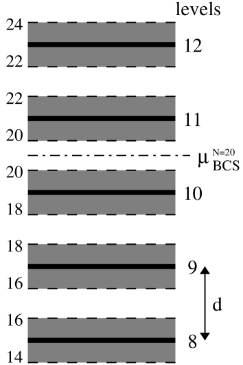
Figure 3: Sketch of the regions of weak and strong pairing for $N=20$. The numbers on the right hand side correspond to the labels of the levels while the ones on the left hand side to the average number of particles of the BCS w.f. at the corresponding $\mu$.

4 NUMERICAL SOLUTION OF THE HILL-WHEELER EQUATION

For our purposes solving the HW equation, Eq. 11, is equivalent to the diagonalization of the Hamiltonian in the nonorthogonal basis of the generator states $|BCS(\xi)\rangle_{N}$. The usual procedure to deal with this equation RS.80 involves two diagonalizations. In a first step, the norm overlap $\mathcal{N}_{\xi\xi^{\prime}}$ is diagonalized

$$\int d\xi^{\prime}\mathcal{N}_{\xi\xi^{\prime}}u_{k}(\xi^{\prime})=n_{k}u_{k}(\xi),$$ (15)

with the functions $u_{k}(\xi)$ forming a complete orthonormal set in the space of the weights $f(\xi)$. Its eigenvalues are never negative, $n_{k}\geq 0$, because the matrix $\mathcal{N}$ is definite positive. We shall keep the $u_{k}(\xi)$ with nonzero eigenvalues corresponding to the linearly independent states. In practice and due to numerical reasons we restrict the $u_{k}(\xi)$ to those with eigenvalues larger than a tolerance $\varepsilon$. For each of these functions there exist states $|k\rangle$,

$$|k\rangle=\frac{1}{\sqrt{n_{k}}}\int d\xi u_{k}(\xi)|BCS(\xi)\rangle_{N},$$ (16)

called the natural states, which span a collective subspace $\mathcal{H}_{C}$. In a second step the Hamiltonian $\hat{H}$ is diagonalized in this space

$$\sum_{k^{\prime}}\langle k|\hat{H}|k^{\prime}\rangle g_{k^{\prime}}=Eg_{k}$$ (17)

with

$$\langle k|\hat{H}|k^{\prime}\rangle=\frac{1}{\sqrt{n_{k}n_{k^{\prime}}}}\int\!\!\!\int d\xi d\xi^{\prime}u_{k}^{\ast}(\xi)\mathcal{H}_{\xi\xi^{\prime}}u_{k^{\prime}}(\xi^{\prime}).$$ (18)

The HW equations provide a set of wave functions,

$$|\Psi^{\sigma}_{N}\rangle=\sum_{k,n_{k}\neq 0}g^{\sigma}_{k}|k\rangle,$$ (19)

and energies $E_{\sigma}$ labeled by the index $\sigma$, the lowest one corresponding to the ground state and the others to excited states. In this work we are only interested in the ground state. Taking into account Eq. 10 and Eq. 19 one obtains

$$f(\xi)=\sum_{k}\frac{g_{k}}{\sqrt{n_{k}}}u_{k}(\xi).$$ (20)

Since the wave functions $|BCS(\xi)\rangle_{N}$ are not orthogonal, the weights $f(\xi)$ cannot be interpreted as the probability amplitude to find the state $|BCS(\xi)\rangle_{N}$ in $|\Psi_{N}\rangle$. It can be shown, however, that the functions

$$\mathcal{G}(\xi)=\sum_{k,n_{k}\neq 0}g_{k}u_{k}(\xi)$$ (21)

are orthogonal and that they can be interpreted as probability amplitudes.

For numerical purposes all the expressions above involving integrals have to be replaced by sums discretizing the space $\xi$. In this form one deals with matrix equations easier to handle. The question that immediately arises is how to determine the optimal $\xi$-mesh to be used in the calculation. The border values of $\xi$ are determined by energy arguments since the probability of mixing high-lying states is very small. The $\xi$-coordinate intervals used in the calculations are given in Table 2. The calculations depend furthermore on the mesh step used in the discretization. This parameter is chosen as to optimize the calculations, i.e., we take the largest mesh that includes all states with relevant information. This parameter is also related to the required accuracy. In the calculations performed we have not attempted to reproduce the exact results up to an unusual accuracy. In Fig. 4 the convergence of the condensation energy, as a function of the number of mesh points used in the calculations, is shown for different numbers of particles and for the coordinates $G$, $\mu$ and $\Delta N^{2}$. We observe that the number of mesh points needed for convergence depends on the $\xi$-coordinate and on the number of particles. The coordinate $G_{trial}$, see top panel, provides the best convergence of the three calculations. For large particle numbers a very good convergence for relatively few mesh points is found. For small numbers of particle one has to go to larger mesh points to find the plateau. For the $\mu$ coordinate the situation is the reverse one, i.e., one finds earlier convergence for small numbers of particles. Finally, the situation for $\Delta N^{2}$ is something in between the two former cases. We find that to reach convergence in energy 80 mesh points are sufficient for all coordinates. This is the number which we will use in all following numerical applications.

Table 2: Initial and final values of the generator coordinates used in the calculations.

N	$20$	$40$	$86$	$172$	$400$
$G_{i}(meV)$	0.44	0.18	0.07	0.03	0.01
$G_{f}(meV)$	0.80	0.30	0.17	0.06	0.04
$\mu_{i}(meV)$	-3.00	-2.00	-2.00	-1.00	-1.00
$\mu_{f}(meV)$	3.00	2.00	2.00	1.00	1.00
$\Delta$N${}^{2}_{i}$	0.00	0.00	0.00	0.00	0.00
$\Delta$N${}^{2}_{f}$	8.00	12.00	16.00	16.00	32.00

Figure 4: The condensation energy in units of $\tilde{\Delta}$ for the three coordinates as a function of the number of mesh points used in the calculations. The energy scales correspond to the N=20 case, the other curves have been shifted in order to make the figure readable. The shifts are 0.28, 0.58, 1.02 and 2.48 for 40, 86, 172 and 400 particles respectively.

A further check concerning the convergence is the number of natural states kept in the calculations. Since many of these states are linearly dependent some natural states $|k\rangle$ will have a vanishing norm and must be excluded. In the calculation only those natural states with a norm larger than a given tolerance $\varepsilon$ are kept. For a given tolerance we take as many states $|k\rangle$ as needed to reach a good plateau. Now we analyze the energy convergence as a function of the number of natural states kept in the diagonalization of the HW equation or equivalently of the tolerance of the calculations. This is shown in Fig. 5 for the three coordinates and for grains with different numbers of particles. In the $\mu$ and $\Delta N^{2}$ coordinates we find that for tolerances smaller than $10^{-10}$ linear dependent states are introduced in the calculations providing unrealistic energy values. The interesting point is the nice plateau found for larger tolerances. The tolerance of $10^{-10}$ corresponds, typically, to around 15 linearly independent states. The coordinate $G$ is in this respect somewhat different. One observes that for tolerances of up to $10^{-15}$ one still gets linearly independent states, which obviously correspond to highly excited states that do not affect the energy of the ground state. This tolerance typically amounts to 20 linearly independent states. From this respect we conclude that if one is interested in excited states the coordinate $G$ is more effective than the other ones.

Figure 5: Same as Fig.4 but as function of the tolerance $\varepsilon$.

The diagonalization of the HW equation in the case of the $\mu$ coordinate requires some comments. As mentioned above in the weak pairing regime, for $N=20$ for example, and for several $\mu$ intervals one does not find superconducting solutions. This circumstance, as explained above, shows up as ”missing points” in the CE curves. These discontinuities do not affect however the solution of the HW equations, since these points have norm zero and do no mix with the other states.

5 APPLICATION TO SUPERCONDUCTING GRAINS

In this section we present a systematic study of properties of superconducting grains. The results of the GCM calculation of different quantities are compared with the PBCS approximation and the exact Richardson solution.

Figure 6: Condensation energies versus the number of particles in different approximations and the exact results. Upper (lower) panel for even (odd) systems.

5.1 Ground State Condensation energies

Condensation energies characterize the presence of pairing correlations. The crossover between superconducting and fluctuation dominated regimes can be described through this quantity.

As in the former cases the condensation energy ${E}_{con}$ is defined as the difference between the total energy in the corresponding approximation and the energy of the uncorrelated Fermi sea. For example in the GCM approaches it is given by ${E}_{con}=E_{\sigma=0}-E_{F}$, see Eq. 19 and below. This quantity is displayed in Fig. 6 for even grains (up to $600$ electrons) and odd grains (up to $601$ electrons) as a function of the particle number $N$. In both plots we give numerical results for the approximations discussed above, BCS, PBCS and the GCMPAV and GCMVAP approaches. The GCMPAV results are presented for the coordinates $G_{trial}$, $\mu$ and $\Delta N^{2}$ and the GCMVAP for $G_{trial}$ and $\Delta N^{2}$. The grand-canonical (BCS) calculation of ${E}_{con}$ predicts vanishing correlations in the few-electron regime in the even and odd systems. The PBCS condensation energies, on the other hand, though always negative predict an unrealistic sharp crossover between the fluctuation dominated regime and the bulk which is more pronounced in odd grains. This artifact is not present neither in the GCM approaches nor in the exact calculations. The simpler GCMPAV approaches already predict a smooth crossover for odd and even grains. The more involved GCMVAP approaches not only predict a smooth crossover but their predictions coincide with the exact results. Concerning the GCMPAV calculations we find that the $\mu$ coordinate is the most effective of all of them followed by the $\Delta N^{2}$ one. Paradoxically the calculation with the $\mu$ coordinate is the simplest one from the numerical point of view.

The reason why the $\mu$ coordinate is the most successful one is probably due to the fact that using this coordinate one has the right inertia parameter for the rotations in the gauge space associated with the operator $\hat{N}$. As a matter of fact this was demonstrated by Peierls and Thouless PT.62 in the context of the translational invariance and a PAV approach by the double projection technique (see Eq.10 above). In this work they show that the right inertia parameter of the collective motion associated with the linear momentum operator $\hat{P}$ ($\hat{N}$ in our case) is obtained when the GCM coordinates are the position ($\varphi$ in our case ) and the velocity ($\mu$ in our case). That means the dynamics associated with Eq. 11 has the right inertial parameter. In a VAP approach one always obtain the right mass parameter RS.80 .

5.2 Pairing correlations.

In a canonical ensemble the BCS order parameter is identically zero. For this reason it is necessary to define another quantity to characterize pair correlations in a state of fixed numbers of electrons. We choose the pairing parameter used in ref.  BD.98

$$\Delta_{b}=G\sum_{k}C_{k}$$ (22)

where the subindex $b$ indicates the number parity of the grain. The quantities $C_{k}$’s are defined by

$$C_{k}^{2}=\langle c_{k+}^{\dagger}c_{k+}c_{k-}^{\dagger}c_{k-}\rangle-\langle c_{k+}^{\dagger}c_{k+}\rangle\langle c_{k-}^{\dagger}c_{k-}\rangle$$ (23)

and form a set of correlators which measure the fluctuations in the occupation numbers. The expectation values $\langle\;\;\rangle$ are to be calculated with the wave functions of the corresponding approach using the formula developed in Appendices A and B. In an uncorrelated or in a blocked state one has $C_{k}=0$. In the grand-canonical case the $C_{k}$’s reduce to $C_{k}=u_{k}v_{k}$ and $\Delta_{b}$ coincides with the usual superconducting order parameter.

Figure 7: The gap parameter $\Delta_{b}$ for the different calculations as a function of the number of electrons for even and odd grains. For particle numbers smaller than those shown in the BCS plot the BCS gap parameter goes sharply to zero.

In Fig. 7 we show our results for the pairing parameter in units of $\tilde{\Delta}$ for even (upper panel) and odd (lower panel) systems respectively. As we can see in both plots the sharp transition occurring in the BCS and PBCS methods is absent in the GCM approaches as well as in the exact solution. The peculiar behaviors of $\Delta_{b}$ in the exact and GCM approximations before and after the BCS breakdown are related to the change of a pairing delocalized in energy (weak pairing regime) to a localized one (strong pairing regime). The rough decrease of $\Delta_{b}$ with $N$ is connected to the special feature of the model, for which the constant $G$ of Eq. (22) is inverse proportional to the number of electrons. The fact that $\Delta_{b}$ converges monotonically to the final value $\tilde{\Delta}$ , in the even case from above and in the odd one from below, is due to the blocking effect. In these plots we observe again that the GCMVAP approaches provide solutions closer to the exact one than the GCMPAV approaches.

5.3 Collective wave functions.

We now look at the structure of the GCM states in the space of the collective parameter $\xi$. The collective weights $f(\xi)$ can not be interpreted as probability amplitudes because the generating states $|BCS(\xi)\rangle_{N}$ are not, in general, orthogonal to each other. The amplitudes $\mathcal{G}(\xi)$ of Eq.(21), on the other hand, play the role of ”collective wave functions”, they are orthogonal and their modules squared have the meaning of a probability.

The quantities $|\mathcal{G}(\xi)|^{2}$ are plotted in Figs. 8, 9 and 10 as a function of the parameters $G$, $\mu$ and $\Delta N^{2}$, respectively. The behavior of $|\mathcal{G}(\xi)|^{2}$ as a function of $\xi$ indicates which are the most relevant components of the states $|\Psi_{N}(\xi)\rangle$ in terms of the parameter $\xi$. To guide the eye we have also plotted in these figures the projected energy $E_{N}(\xi)$ of Eq. (6). For simplicity we restrict our discussion to even systems. In Fig. 8 we represent these quantities for the coordinate $G_{trial}$ in the GCMPAV and GCMVAP approaches. Since the wave functions of both approaches do not differ qualitatively we shall discuss both cases together. The fact that the projected energies are lower in the PAV than in the VAP approach for a given $G_{trial}-G_{c}$ is due to the fact that $G_{c}$ is almost zero for all particle numbers in the VAP approach while it varies considerably with the particle number for the PAV case, see Table 2. We find broad potential energy curves for small particle numbers and narrower ones with increasing $N$. Interestingly the potential energy curves for the GCMPAV and GCMVAP approaches are rather different for small particle numbers and they become similar for the large ones. Concerning the wave functions for $N=20$ we obtain very broad distributions corresponding to a situation of weak pairing dominated by fluctuations in the order parameter $\Delta$, see also panel a) of Fig. 2. For $N\sim 40$ we find that the wave functions are not that extended anymore but they still present a two peak distribution, wit the first peak around the non-superconducting solution and the other around a superconducting one. For larger particle numbers ($N\sim 86,172,400$) a one peak distribution emerges with the width of the peak getting smaller for increasing particle number. Looking at Fig. 2a we see that at large $N$ the distribution peaks around the wave function with a gap very close to the bulk one.

Figure 8: The projected energies $E_{N}(G)$ versus $G$ in the GCMPAV (thin continuous lines) and GCMVAP (thick continuous lines) approaches for even systems. The collective wave functions $|\mathcal{G}(G)|^{2}$ for the GCMPAV (thin dashed lines) and the GCMVAP (thick dashed lines) approaches in arbitrary units. The vertical scale applies for $E_{N}(G)$, the minimum of $E_{N}(G)$ in each approach has been set equal to zero. The top scale applies only for the top panel.

The results for the $\mu$ coordinate are presented in Fig. 9. For $N=20$, in the weak pairing region, we obtain a flat potential which shape corresponds to the physics already discussed in relation with Fig. 3. The collective wave function, also according to the discussion of Fig. 2b and Fig. 3, displays an oscillating behavior with maxima around $\mu=kd$ and minima (zeroes) around $\mu=k(d+1/2)$. The height of the maxima decreases considerably for $k$ values different from 10 and 11, i.e., the collective wave function is mainly formed by the HF solution around the Fermi level and the N=20 components of the BCS solution of the levels above and below the Fermi level. For $N=40$ the weak pairing regime persists and the wave function displays a structure similar to the $N=20$ case but with the strength much more concentrated owing to the fact that the level spacing decreases with increasing number of particles. For $N=86$ the two peak structure is just a reminiscence of the weak pairing situation and for $N=172$ and 400 a one peak structure emerges indicating the strong pairing situation. The potential energy curves get steeper with increasing N and the localization of the peak around $\mu^{N}_{BCS}$ sharpens in the same way. As one can see in Fig. 2b the range of the $\Delta$ parameter covered by the wave functions diminishes with increasing $N$.

Figure 9: The projected energies $E_{N}(\mu)$ (continuous lines) and the collective wave functions $|\mathcal{G}(\mu)|^{2}$ ( dashed lines) versus $\mu$. The vertical scale applies for $E_{N}(\mu)$, the minimum of $E_{N}(\mu)$ has been set equal to zero. $|\mathcal{G}(\mu)|^{2}$ is in arbitrary units. The top scale applies only for the top panel.

Lastly we discuss the $\Delta N^{2}$ coordinate in Fig. 10. The potential energy curves are easy to understand. In the small particle number limit the BCS solution does not provide a superconducting solution and therefore $\langle\Delta N^{2}\rangle=0$. On the other hand the BCS approximation provides the exact solution in the bulk limit, i.e. there $\langle\Delta N^{2}\rangle>>1$. Accordingly we expect minima in the projected energies at small $\Delta N^{2}$ for low N and at large $\Delta N^{2}$ for large N. The potential energy curves get softer with growing N because for increasing $\Delta N^{2}$ it is energetically easier to change this value. As it should be the potential energy curve for the GCMVAP approach lies below the GCMPAV one. Concerning the collective wave functions, their behaviors correspond to the shape of the potentials. For $N\leq 86$ there is a finite probability of having an uncorrelated HF solution as a component of the collective wave functions and only for $N\geq 172$ we obtain Wigner-like functions with zero amplitude for the HF component. The range of $\Delta$’s covered by the wave functions can be read from Fig. 2c.

Finally, we would like to mention that a very detailed comparison of our wave functions and the exact ones has been made in ref. FE.03 . We find that the physical content of the GCMPAV wave functions and the exact ones is identical.

Figure 10: The same as in figure 8 but for the parameter $\Delta N^{2}$.

6 Conclusions

In this paper we have presented a detailed formulation of the particle number projected Generator Coordinate Method. We have discussed two different coordinates to generate wave functions for the variation after projection method and three for the projection after variation one. The theory has been applied to study superconducting grains with a pairing Hamiltonian. We have shown that the GCMVAP calculations with both proposed coordinates reproduce the exact results in the weak, crossover and bulk regimes. Concerning the GCMPAV calculations we find that all three proposed coordinates, in spite of not being able to reproduce the exact results, describe qualitatively the correct physics washing out the phase transition found in the BCS and the PBCS approaches. Concerning the degree of accuracy we find that the $\mu$ coordinate is the most effective of all the three followed by the $\Delta N^{2}$ one.

We think that these results are rather general and apply to many more complex Hamiltonians than the naive pairing one considered here. Since the GCM Ansatz includes explicitly fluctuations in the wave function it is very appropriate to deal with finite systems where phase transitions may take place. The method, contrary to other approximations, applies equally well to systems with very few or very large particle number. On the other hand the GCM Ansatz is very versatile to be adapted to other physical situations by considering additional coordinates to the ones discussed in this work.

This work has been supported in part by DGI, Ministerio de Ciencia y Tecnología, Spain, under Project FIS2004-06697. M.A.F. acknowledges a scholarship of the Programa de Formacion del Profesorado Universitario (Ref. AP2002-0015)

Appendix A Peculiarities of the PBCS approximation

In this appendix we discuss some numerical aspects of the solution of the equations used in this article.

A.1 Odd particle number case

The PBCS and HW methods can be extended to systems with an odd number of particles by blocking one of the available states. A system with an odd particle number is described by the state

$$|BCS\rangle_{N+1}^{l} = \int_{0}^{2\pi}\frac{d\varphi}{2\pi}e^{iN\varphi}c^{\dagger}_{l}$$ (24)

$$\times \prod_{k\neq l}(e^{-i\varphi/2}u_{k}+e^{i\varphi/2}v_{k}c^{\dagger}_{k+}c^{\dagger}_{k-})|-\rangle$$

with $N$ an even number and $l$ the blocked state. The residuum integral of Eq. (4) now looks like

$${}^{l}R_{m}^{j_{1},\cdots,j_{M}} = \frac{1}{2\pi}\int_{0}^{2\pi}d\varphi\,e^{-i(M-2m)\varphi/2}$$ (25)

$$\times \prod_{k\neq j_{1},\cdots,j_{M},l}^{N}(e^{-i\varphi/2}u_{k}^{2}+e^{i\varphi/2}v_{k}^{2}),$$

in an obvious notation. As before all expectation values can easily be calculated in terms of the residuum integrals, for example the norm matrix element is given by

$${}_{N+1}\langle BCS|BCS\rangle_{N+1}={{}^{l}R}_{0}^{0},$$ (26)

and the projected energy by

$$E_{N+1}^{l} = 2\sum_{j(\neq l)=1}^{N}\left(\epsilon_{j}-\frac{G}{2}\right)v_{j}^{2}\frac{{}^{l}R_{1}^{j}}{{}^{l}R_{0}^{0}}$$

$$- G\sum_{j,k\neq l}^{N}u_{j}v_{j}u_{k}v_{k}\frac{{}^{l}R_{1}^{jk}}{{}^{l}R_{0}^{0}}+\epsilon_{l}.$$

The superindex is somewhat superfluous and it can be suppressed. Blocking different states $l$ one obtains different excited states. The lowest of these energies corresponds to the ground state of the system with an odd particle number. The PBCS and HW variational equations obtained with theses states can be guessed without further calculations: In all sums and products in the equations presented for even systems the term corresponding to the blocked state $l$ has to be excluded. In the same way one can write down states with 3,5,.. etc. blocked states.

A.2 Numerical solution of the PBCS equations.

The set of coupled non-linear equations (7) is usually solved by an iterative procedure. In order to speed up such procedure it is convenient to introduce the variable $\chi_{k}$ through the relation

$$u_{k}^{2}=\frac{\chi_{k}}{1+\chi_{k}},\,\,\,\,\,v_{k}^{2}=\frac{1}{1+\chi_{k}},$$ (27)

where the normalization condition $u_{k}^{2}+v_{k}^{2}=1$ has been taken into account by construction. In terms of $\chi_{k}$ the variational equations look like

$$\left(\hat{\epsilon}_{k}+\Lambda_{k}\right)\chi_{k}^{1/2}-\Delta_{k}\left(\chi_{k}-1\right)=0.$$ (28)

The additional transformation

$$\chi_{k}=\exp{\theta_{k}}$$ (29)

allows to isolate the new variable in terms of the fields $\hat{\epsilon}_{k},\Lambda_{k}$ and $\Delta_{k}$

$$\theta_{k}=2\sinh^{-1}\left(\frac{\hat{\epsilon}_{k}+\Lambda_{k}}{2\Delta_{k}}\right).$$ (30)

The right hand side of this equation does not depend explicitly on $\theta_{k}$ because the fields $\hat{\epsilon}_{k},\Lambda_{k}$ and $\Delta_{k}$ are independent of $\theta_{k}$. This fact is very useful to solve Eq. (30) by numerical iteration. We start with a guess of $\theta_{k}$ (for instance the grand-canonical solution) and solve (30) until the convergence of the energy, to a given tolerance, has been reached.

The variational equations (30) involve the computation of the residuum integrals $R_{n}^{\nu_{1}\ldots\nu_{M}}$. These integrals can be calculated analytically using the existing closed analytical expression TM.99 . Their evaluation, however, requires the addition of many terms making the whole computation a very time consuming approach. As the integrals must be computed many times for different sets of $u_{k},v_{k}$, the numerical solution of (30) in an efficient way requires the computation of the residuum integrals in a fast and accurate way. For this purpose we have implemented Fast Fourier Transform routines to evaluate the integrals reducing the number of different integrals as much as possible to minimize the computational effort. For this purpose the following two identities can be used. The first one was found by Dietrich et al DM.64 . It can be shown that the residuum integrals satisfy the following recursion relation

$$R_{m}^{j_{1},\cdots,j_{M}}=u_{k}^{2}R_{m}^{j_{1},\ldots,j_{M},k}+v_{k}^{2}R_{m+1}^{j_{1},\ldots,j_{M},k}$$ (31)

The knowledge of two residuum integrals allows to calculate a different one. This reduces the number of numerical integrations by one third. A second, more powerful relation was found by Ma and Rasmussen MR.77 ,

$$R_{m}^{j_{1},\ldots,j_{M}} = \delta_{m,M}R_{0}^{0}\!\!\!\!\!\!\!\!\prod_{j=j_{1},\ldots,j_{M}}\frac{1}{v_{j}^{2}}+(-)^{m}\!\!\!\!\!\!\!\sum_{j=j_{1},\ldots,j_{M}}\!\!\!\!\!\!v_{j}^{2(M-m-1)}u_{j}^{2m}$$ (32)

$$\times \left(\prod_{k=j_{1},\ldots,j_{M}(\neq j)}\frac{1}{v_{j}^{2}-v_{k}^{2}}\right)R_{0}^{j}.$$

This formula allows to calculate all residuum integrals if the integrals $R_{0}^{0}$ and $R_{0}^{j}$ are known. This relation reduces to $N+1$ the overall number of numerical integrations for a given set of $v_{j}$’s and $u_{j}$’s.

In the PBCS one only needs Ma’s relation to calculate three terms: $R_{1}^{jk}$,$R_{2}^{jkl}-R_{1}^{jkl}$ and $R_{2}^{jk}-R_{1}^{jk}$. If $R_{0}^{0}$ and $R_{0}^{j}$ are known, $R_{1}^{j}$ can be obtained by Dietrich’s recursion relation. First we consider $R_{m}^{jk}$ with $m=1$ or $m=2$. Ma and Rasmussen’s formula reduces to

$$R_{m}^{jk}=\delta_{m,2}\frac{R_{0}}{v_{j}^{2}v_{k}^{2}}+(-)^{m}\frac{\zeta_{j}^{m}v_{j}^{2}R_{0}^{j}-\zeta_{k}^{m}v_{k}^{2}R_{0}^{k}}{v_{j}^{2}-v_{k}^{2}}$$ (33)

where we have used the identity $\zeta_{j}=\frac{1}{v_{j}^{2}}-1$. The difference $R_{2}^{jk}-R_{1}^{jk}$ can be written in a simplified way as follows

$$R_{2}^{jk}-R_{1}^{jk}=\frac{R_{0}}{v_{j}^{2}v_{k}^{2}}-\frac{R_{0}^{j}(v_{j}^{2}-1)}{v_{j}^{2}(v_{j}^{2}-v_{k}^{2})}+\frac{R_{0}^{k}(v_{k}^{2}-1)}{v_{k}^{2}(v_{j}^{2}-v_{k}^{2})}$$ (34)

The calculation of $R_{2}^{jkl}-R_{1}^{jkl}$ is a bit more complicated, the result is

$$R_{2}^{jkl}-R_{1}^{jkl} = \frac{u_{j}^{4}+u_{j}^{2}v_{j}^{2}R_{0}^{j}}{(v_{j}^{2}-v_{k}^{2})(v_{j}^{2}-v_{l}^{2})}+\frac{u_{k}^{4}+u_{k}^{2}v_{k}^{2}R_{0}^{k}}{(v_{k}^{2}-v_{j}^{2})(v_{k}^{2}-v_{l}^{2})}+$$ (35)

$$+ \frac{u_{l}^{4}+u_{l}^{2}v_{l}^{2}R_{0}^{l}}{(v_{l}^{2}-v_{j}^{2})(v_{l}^{2}-v_{k}^{2})}.$$

Since the indices of the residuum integrals can be permuted, $R_{2}^{jkl}-R_{1}^{jkl}$ can be expressed for all possible combinations of $v_{j},v_{k},v_{l}$ by the equations above.

Appendix B The generalized residuum integrals

The Hamiltonian overlap $\mathcal{H}_{\xi\xi^{{}^{\prime}}}$, Eq. (12), can be calculated using the generalized Dietrich’s recursion relation,

$$R_{m}^{j_{1}\cdots j_{M}}(\xi,\xi^{\prime}) = u_{k}(\xi)u_{k}(\xi^{\prime})R_{m}^{j_{1}\cdots j_{M},k}(\xi,\xi^{\prime})+$$ (36)

$$+ v_{k}(\xi)v_{k}(\xi^{\prime})R_{m+1}^{j_{1}\cdots j_{M},k}(\xi,\xi^{\prime})$$

The residuum integrals $R_{1}^{i},R_{1}^{ij}$ needed to calculate $\mathcal{H}_{\xi\xi^{{}^{\prime}}}$ can be written in terms of $R_{0}^{j}$ and $R_{0}^{jk}$ using Dietrich’s relation twice

$$R_{1}^{k}(\xi,\xi^{\prime})=\frac{R_{0}^{0}(\xi,\xi^{\prime})-u_{k}(\xi)u_{k}(\xi^{\prime})R_{0}^{k}(\xi,\xi^{\prime})}{v_{k}(\xi)v_{k}(\xi^{\prime})}$$ (37)

$$R_{1}^{jk}(\xi,\xi^{\prime})=\frac{R_{0}^{j}(\xi,\xi^{\prime})-u_{k}(\xi)u_{k}(\xi^{\prime})R_{0}^{jk}(\xi,\xi^{\prime})}{v_{k}(\xi)v_{k}(\xi^{\prime})}.$$ (38)

The calculation of the Hamiltonian overlap using this method is rather slow. In order to speed up the evaluation of the residuum integrals, we have written the Hamiltonian overlap $\mathcal{H}_{\xi\xi^{{}^{\prime}}}$ in the form

$$\mathcal{H}_{\xi\xi^{{}^{\prime}}}=\frac{1}{2\pi}\int_{0}^{2\pi}\!\!d\varphi\,[F_{1}^{\varphi}(\xi,\xi^{{}^{\prime}})-F_{2}^{\varphi}(\xi,\xi^{{}^{\prime}})]$$ (39)

where

$$F_{1}^{\varphi}(\xi,\xi^{{}^{\prime}})=2\sum_{j}(\epsilon_{j}-G/2)v_{j}(\xi)v_{j}(\xi^{{}^{\prime}})e^{i\varphi/2}$$ (40)

$$\times \prod_{k\neq j}(e^{-i\varphi/2}u_{k}(\xi)u_{k}(\xi^{{}^{\prime}})+e^{i\varphi/2}v_{k}(\xi)v_{k}(\xi^{{}^{\prime}}))$$

$$F_{2}^{\varphi}(\xi,\xi^{{}^{\prime}})=G\sum_{ij}u_{i}(\xi^{{}^{\prime}})v_{i}(\xi)u_{j}(\xi)v_{j}(\xi^{{}^{\prime}})$$ (41)

$$\times \prod_{k\neq ij}(e^{-i\varphi/2}u_{k}(\xi)u_{k}(\xi^{\prime})+e^{i\varphi/2}v_{k}(\xi)v_{k}(\xi^{\prime})).$$

In the actual calculations we used these expressions to evaluate $\mathcal{H}_{\xi\xi^{{}^{\prime}}}$ instead of Eqs. (37)(38), the integrals 39 are evaluated by fast Fourier routines.

References

- (1) C. T. Black and D. C. Ralph and M. Tinkham, Phys. Rev. Lett. 76, (1996) 688.
- (2) C. T. Black and D. C. Ralph and M. Tinkham, Phys. Rev. Lett. 78, (1997) 4087.
- (3) A. Mastellone and G. Falci and R. Fazio, Phys. Rev. Lett. 80, (1998) 4542.
- (4) J. Dukelsky and G. Sierra, Phys. Rev. Lett. 83, (1999) 172
- (5) J. Von Delft, Annalen der Physik 3, (2001) 219. .
- (6) R. W. Richardson and N. Sherman, Nucl. Phys. 52, (1964) 221.
- (7) M. Schechter, Y. Imry and Y. Levinson, Phys. Rev. B 63, (2001) 214518.
- (8) G. Falci, R. Fazio, G. Giaquinta, A. Mastellone, Philos. Mag. B 80, (2000) 883
- (9) R. Rossignoli, N. Canosa and J. L. Egido, Phys. Rev. B 64, (2001) 224511.
- (10) E. Yuzbashyan, A. A. Baytin and B. L. Altshuler, Phys. Rev. Lett. 71, (2005) 094504.
- (11) F. Braun and J. von Delft, Phys. Rep. 59, (1999) 9527.
- (12) J. Dukelsky and C. Esebbag and P. Schuck, Phys. Rev. Lett. 87, (2001) 066403.
- (13) M. A. Fernandez and J. L. Egido, Phys. Rev. B 68, (2003) 184505.
- (14) D. Hill and J. A. Wheeler, Phys. Rev. 89, (1953) 1102.
- (15) M.A. Fernandez and J.L. Egido, to be published.
- (16) J. Bardeen and L. N. Cooper and J. R. Schrieffer, Phys. Rev. 108, (1957) 1175.
- (17) K. Dietrich and H. J. Mang and J. H. Pradal, Phys. Rev. 135, (1964)
- (18) F. Braun and J. von Delft, Phys. Rev. Lett. 81, (1998) 4712.
- (19) F. Braun and J. von Delft, Phys. Rev. B59, (1999) 9527.
- (20) P. W. Anderson, Phys. Rev. 112, (1958) 1900.
- (21) P. Ring and P. Schuck, The Nuclear Many Body Problem (Springer-Verlag, Berlin 1980)
- (22) R.E. Peierls and J. Yoccoz, Proc. Phys. Soc. A70, (1957) 381
- (23) R.E. Peierls and D.J. Thouless, Nucl. Phys. 38, (1962) 154
- (24) B. Jancovici and D.H. Schiff, Nucl. Phys. 58, (1964) 678
- (25) K. Tanaka and F. Marsiglio, Phys. Rev. B 60, (1999) 3508.
- (26) Chin W. Ma and John O. Rasmussen, Phys. Rev. C 16, (1977)