Theory of Interacting Bloch Electrons in a Magnetic Field

Abstract

We study interacting electrons in a periodic potential and a uniform magnetic field ${\mib B}$ taking the spin-orbit interaction into account. We first establish a perturbation expansion for those electrons with respect to the Bloch states in zero field. It is shown that the expansion can be performed with the zero-field Feynman diagrams of satisfying the momentum and energy conservation laws. We thereby clarify the structures of the self-energy and the thermodynamic potential in a finite magnetic field. We also provide a prescription of calculating the electronic structure in a finite magnetic field within the density functional theory starting from the zero-field energy-band structure. On the basis of these formulations, we derive explicit expressions for the magnetic susceptibility of ${\mib B}\!\rightarrow\!{\mib 0}$ at various approximation levels on the interaction, particularly within the density functional theory, which include the result of Roth [J. Phys. Chem. Solids 23 (1962) 433] as the non-interacting limit. We finally study the de Haas-van Alphen oscillation in metals to show that quasiparticles at the Fermi level with the many-body effective mass are directly relevant to the phenomenon. The present argument may be more transparent than that by Luttinger [Phys. Rev. 121 (1961) 1251] of using the gauge invariance and has an advantage that the change of the band structure with the field may be incorporated.

1 Introduction

Extensive theoretical studies have been carried out on Bloch electrons in a magnetic field ${\mib B}$ which display many exciting phenomena. Among them are investigations on fundamental quantities and phenomena such as the effective Hamiltonian,[1, 2, 3, 4, 5, 6, 7, 8, 9] the static magnetic susceptibility,[1, 10, 11, 12, 4, 5, 13, 14, 15, 16, 17, 18, 19, 20, 21, 22, 23, 24, 25, 26, 27, 28, 29, 30, 31, 32, 33, 34, 35] and the de Haas-van Alphen (dHvA) oscillation.[36, 37, 38, 39, 15, 40, 41] Since the relevant energy scale is $\mu_{\rm B}B\!\lesssim\!1$meV with $\mu_{\rm B}$ the Bohr magneton, it seems natural to start from the energy-band structure in zero field and try to include the field effects perturbatively. However, a uniform magnetic field in quantum mechanics necessarily accompanies a vector potential with a non-periodic linear spatial dependence. Hence the procedure is not at all an easy task to perform as it apparently looks, particularly when the electron-electron interaction is taken into account. For example, we still do not have a satisfactory calculation of the total magnetic susceptibility of metals, even for Li and Na.

The purposes of the present paper are threefold. We first establish a definite theoretical prescription to calculate properties of interacting Bloch electrons in a uniform magnetic field on the basis of the energy-band structure in zero field. This includes an extension of the density functional theory[42, 43, 44, 45, 46, 47, 48, 49, 50, 51, 52, 53, 54] to a finite magnetic field. We then derive explicit expressions of the total magnetic susceptibility $\chi({\mib B}\!\rightarrow\!{\mib 0})$ at various approximation levels on the electron-electron interaction. Finally, the formulation is used to study many-body effects on the dHvA oscillation in metals.

Let us briefly summarize the relevant works on the effective Hamiltonian, the density functional theory, the magnetic susceptibility and the dHvA oscillation together with the extensions considered here.

We now have a well-established effective Hamiltonian in a uniform magnetic field at the one-particle level;[1, 2, 3, 4, 5, 8] see also Ref. Nenciu91 on mathematical aspects. Let $t^{(0)}({\mib R}\!-\!{\mib R}^{\prime})$ denote the transfer integral in zero field between two unit cells specified by ${\mib R}$ and ${\mib R}^{\prime}$; it completely determines the energy-band structure.[55] Then the transfer integral in a finite field is obtained by the replacement:

$$t^{(0)}({\mib R}\!-\!{\mib R}^{\prime})\longrightarrow{\rm e}^{iI_{{\mib R}{\mib R}^{\prime}}}\,t({\mib R}\!-\!{\mib R}^{\prime},{\mib B})\,,$$ (1a)

where $$I_{{\mib R}{\mib R}^{\prime}} t({\mib R}\!-\!{\mib R}^{\prime},{\mib B}\!\rightarrow\!{\mib 0})\!\rightarrow\!t^{(0)}({\mib R}\!-\!{\mib R}^{\prime}) {\mib B} t {\mib B} t {\cal E}^{(0)}({\mib k})\!\rightarrow\!{\cal E}\!\left(-i{\mib\nabla}\!-\!\frac{e}{\hbar c}{\mib A}\right) {\cal E}^{(0)}({\mib k}) {\mib k} {\mib A}$$ is the Peierls phase[1] and . The relation was first obtained by Peierls[1] for the tight-binding model without the dependence in . The extension beyond the tight-binding model is due to Luttinger.[2] The dependence in was taken into account by Kohn,[3] Blount,[4] and Roth.[5] As shown by Luttinger,[2] eq. (1a) provides a microscopic justification for the procedure: with an energy eigenvalue in zero field, a wave vector in the first Brillouin zone, and the vector potential, which was a key assumption in the Onsager-Lifshitz-Kosevich theory for the dHvA oscillation.[36, 37] Here, we also consider interaction effects on the basis of the treatments by Luttinger[2] and Roth.[5] It is thereby shown that the self-energy also experiences the change:

$$\Sigma^{(0)}(\varepsilon_{n},{\mib R}\!-\!{\mib R}^{\prime})\longrightarrow{\rm e}^{iI_{{\mib R}{\mib R}^{\prime}}}\,\Sigma(\varepsilon_{n},{\mib R}\!-\!{\mib R}^{\prime},{\mib B})\,,$$ (1b)

with $\varepsilon_{n}$ the Matsubara frequency. We will provide a definite prescription of how to calculate $\Sigma(\varepsilon_{n},{\mib R}\!-\!{\mib R}^{\prime},{\mib B})$ for an arbitrary finite field ${\mib B}$. Thus, our approach is more powerful than those by the expansion in ${\mib A}$[19, 23] that is effective only in the zero-field limit. With an application to superconductors in mind, the whole formulation will be carried out without assuming a specific gauge for the vector potential in such a way that an extension to a non-uniform magnetic field may be performed easily.

The density functional theory (DFT) is regarded now as one of the most efficient and reliable methods for the quantitative understanding of solids.[52, 54] Its extension to a finite magnetic field has been performed by Vignale and Rasolt[51] using the current density ${\mib j}({\mib r})$ as the relevant extra variable, and also by Grayce and Harris[53] choosing ${\mib B}$ instead of ${\mib j}({\mib r})$. In these formulations, however, one has to calculate the electronic structure in ${\mib B}$ from the beginning by treating the field and the periodic potential on an equal footing. Thus, practical calculations for solids have never been carried out. Here, we will provide a prescription of obtaining the electronic structure in ${\mib B}$ within DFT based on the known zero-field energy-band structure. This two-step procedure may be regarded as one of the main advantages of the present formulation over the previous ones.[51, 53] We choose the average flux density ${\mib B}\!\equiv\!{\mib\nabla}\!\times\!{\mib A}$ as the relevant variable. The total moment may be obtained by ${\mib M}\!=\!-(\partial\Omega/\partial{\mib B})$, and the external field is found by ${\mib H}\!=\!{\mib B}\!-\!4\pi{\mib M}/V$ with $V$ the volume.

The static magnetic susceptibility $\chi({\mib B}\!\rightarrow\!{\mib 0})$ has been a matter of extensive theoretical investigations,[1, 10, 11, 12, 4, 5, 13, 14, 15, 16, 17, 18, 19, 20, 21, 22, 23, 24, 25, 26, 27, 28, 29, 30, 31, 32, 33, 34, 35] and we now have several apparently different but essentially equivalent expressions of $\chi$ for non-interacting Bloch electrons.[5, 13, 14, 20] Among them, Roth[5] gave a complete expression including the spin-orbit interaction with a clear derivation process. We closely follow her procedure to extend the consideration into interacting Bloch electrons. It should be noted that $\chi$ of interacting Bloch electrons were already calculated for the orbital part by by Fukuyama,[19] Phillipas and McClure,[21] and Fukuyama and McClure,[23] and for both the orbital and spin parts by Buot[28] and Misra et al.[31] However, most of them provided only approximate treatments of $\chi$: either the vertex corrections were neglected[19, 23, 31] or the frequency dependence of the self-energy were not considered.[21, 31] Also, the treatment by Buot[28] fails to incorporate vertex corrections explicitly in the general expression. We here present a complete framework to calculate $\chi$ at various approximation levels on the interaction. Particularly, we derive an explicit expression of $\chi$ within DFT. Calculations of the susceptibility by DFT have been performed only for the spin part,[24, 25, 26, 29, 34, 35] for the orbital part neglecting vertex corrections,[27, 30, 32] and for the both parts but neglecting vertex corrections.[33] Thus, there is no available expression within DFT for the total susceptibility with vertex corrections. The formula obtained here, which incorporates the effects of the spin-orbit interaction, core polarizations, interband transitions, and vertex corrections, is expected to enhance our understanding on the total magnetic susceptibility of solids. It will be shown that the vertex corrections of the spin part in our formula naturally include the Stoner enhancement factor.[10, 56]

The dHvA oscillation in metals provides unique information on the Fermi-surface structures and interaction effects. The classic theory at the one-particle level is due to Lifshitz and Kosevich,[37] who applied Onsager’s semiclassical quantization scheme[36] to non-interacting band electrons. The interaction effects were considered by Luttinger[38] and Bychkov and Gor’kov.[39] However, Bychkov and Gor’kov considered only an isotropic Fermi liquid. Also, the work by Luttinger[38] is based on a gauge-invariance argument ${\cal E}^{(0)}({\mib k})\!+\!\Sigma^{(0)}(\varepsilon_{n},{\mib k})\!\rightarrow\!{\cal E}\!\left(-i{\mib\nabla}\!-\!\frac{e}{\hbar c}{\mib A}\right)\!+\!\Sigma\!\left(\varepsilon_{n},-i{\mib\nabla}\!-\!\frac{e}{\hbar c}{\mib A}\right)$ without clarifying the structure of the self-energy explicitly. Hence it is not clear from Luttinger’s argument whether it is the momentum ${\mib p}$ or the crystal momentum $\hbar{\mib k}$ in the first Brillouin zone that is really relevant. The replacement procedure for the self-energy needs to be established microscopically in the same sense as eq. (1a) had to. His argument also has an ambiguity as to the “non-oscillatory part” of the self-energy, which later caused an interpretation[40, 41] that the self-energy does not participate in making up the quantized energy levels, i.e., one only has to replace the one-particle part as ${\cal E}^{(0)}({\mib k})\!\rightarrow\!{\cal E}\!\left(-i{\mib\nabla}\!-\!\frac{e}{\hbar c}{\mib A}\right)$. To remove the confusion and also to analyze experiments unambiguously, it will be well worth placing the theory on a firm ground. On the basis of the formulation to derive eq. (1b), we will present a hopefully clearer argument for the many-body effects on the dHvA oscillation. This argument also has an advantage that the change of the energy-band structure with the field can be taken into account.

This paper is organized as follows. Section 2 provides an alternative derivation of the effective one-particle Hamiltonian with the spin-orbit interaction. We combine the advantages in the treatments of Luttinger[2] and Roth[5] to formulate the problem so that extensions (i) to interacting systems and (ii) to a non-uniform magnetic field may be performed easily. Section 3 takes the electron-electron interaction into account. We establish a perturbation expansion for the thermodynamic potential and the self-energy in terms of the energy-band structure in zero field. It is shown that only the zero-field Feynman diagrams are necessary. We also construct a DFT in a finite magnetic field. Section 4 derives expressions of the magnetic susceptibility at various approximation levels, including that of DFT. Section 5 studies many-body effects on the dHvA oscillation in metals. Section 6 summarizes the paper. We put $k_{\rm B}\!=\!1$ throughout.

2 Effective Hamiltonian

2.1 Hamiltonian and basis functions

We consider Bloch electrons in a uniform magnetic field described by a Hamiltonian with the spin-orbit interaction and Pauli paramagnetism:

$$\hat{\cal H}=\frac{\hat{\mib P}^{2}}{2m}+{\cal V}({\mib r})-g\frac{e\hbar}{2m^{2}c^{2}}(\hat{\mib s}\times{\mib\nabla}{\cal V})\cdot\hat{\mib P}-g\frac{e\hbar}{2mc}\hat{\mib s}\cdot{\mib B}-\mu\,.$$ (2)

Here $m$ and $e(<\!\!0)$ are the electron mass and charge, respectively, $\hat{\mib P}$ is defined by

$$\hat{\mib P}\equiv\hat{\mib p}-\frac{e}{c}{\mib A}({\mib r})\,,$$ (3)

with $\hat{\mib p}$ the momentum operator and ${\mib A}({\mib r})$ the vector potential, ${\cal V}({\mib r})$ denotes the periodic lattice potential, $g$ is the electron $g$ factor, $\hat{\mib s}$ is the dimensionless spin operator, ${\mib B}\!\equiv\!{\mib\nabla}\!\times\!{\mib A}({\mib r})$ is the magnetic field, and $\mu$ is the chemical potential.

The eigenfunctions of eq. (2) at ${\mib A}\!=\!{\mib 0}$ are the Bloch spinors:

$$\vec{\psi}_{b{\mib k}}({\mib r})={\rm e}^{i{\mib k}\cdot{\mib r}}\,\vec{u}_{b{\mib k}}({\mib r})\,,$$ (4)

where ${\mib k}$ is a wave vector in the first Brillouin zone and $b$ denotes a set of quantum numbers for the band and spin. They are orthonormal as $\langle\vec{\psi}_{b{\mib k}}|\vec{\psi}_{b^{\prime}{\mib k}^{\prime}}\rangle\!=\!\delta_{bb^{\prime}}\delta_{{\mib k}{\mib k}^{\prime}}$ and form a complete set. For our consideration, however, the wave functions (4) may not necessarily be the eigenfunctions of eq. (2) at ${\mib A}\!=\!{\mib 0}$. Thus, we will proceed by assuming only the completeness and orthonormality of eq. (4). Note that, relaxing the conditions in this way, $\vec{\psi}_{b{\mib k}}({\mib r})$ may be chosen analytic in ${\mib k}$ throughout the Brillouin zone, as shown by des Cloizeaux[57, 58] and Nenciu.[59, 9] Those basis functions, which are analytic in ${\mib k}$ but not necessarily the eigenfunctions of $\hat{\cal H}$, were named quasi-Bloch functions by des Cloizeaux.[57, 58]

A set of alternative basis functions was introduced by Wannier,[60] which are more suitable for the present purpose. They are defined as a Fourier transform of $\vec{\psi}_{b{\mib k}}({\mib r})$ by

$$\vec{w}_{b{\mib R}}({\mib r})\equiv\frac{1}{\sqrt{N_{\rm c}}}\sum_{\mib k}{\rm e}^{-i{\mib k}\cdot{\mib R}}\,\vec{\psi}_{b{\mib k}}({\mib r})\,,$$ (5)

where ${\mib R}$ specifies a unit cell and $N_{\rm c}$ denotes the number of unit cells in the system. It hence follows that the Wannier functions are also complete $\sum_{b{\mib R}}|\vec{w}_{b{\mib R}}\rangle\langle\vec{w}_{b{\mib R}}|\!=\!1$ and orthonormal as $\langle\vec{w}_{b{\mib R}}|\vec{w}_{b^{\prime}{\mib R}^{\prime}}\rangle\!=\!\delta_{bb^{\prime}}\delta_{{\mib R}{\mib R}^{\prime}}$ with $\vec{w}_{b{\mib R}}({\mib r})\!=\!\vec{w}_{b{\mib 0}}({\mib r}\!-\!{\mib R})$.

To describe Bloch electrons in a finite magnetic field, we adopt the basis functions introduced by Luttinger.[2] They differ from eq. (5) by only a phase factor as

$$\vec{w}_{b{\mib R}}^{\,\prime}({\mib r})={\rm e}^{iI_{{\mib r}{\mib R}}}\vec{w}_{b{\mib R}}({\mib r})\,,$$ (6a)

where $$I_{{\mib r}{\mib R}}$$ is defined by

$$I_{{\mib r}{\mib R}}\equiv\frac{e}{\hbar c}\int_{{\mib R}}^{{\mib r}}{\mib A}({\mib r}^{\prime})\cdot{\rm d}{\mib r}^{\prime}\,,$$ (6b)

with ${\rm d}{\mib r}^{\prime}$ taken along the straight line path from ${\mib R}$ to ${\mib r}$. We assume that the functions $\{\vec{w}_{b{\mib R}}^{\,\prime}\}$ form a complete set, although they are not orthonormal in a finite magnetic field. This latter inconvenience can be removed by considering the linear combination:

$$\vec{\varphi}_{b{\mib R}}({\mib r})=\sum_{b^{\prime}}\sum_{{\mib R}^{\prime}}{\cal S}_{b^{\prime}{\mib R}^{\prime},b{\mib R}}\,\vec{w}_{b^{\prime}{\mib R}^{\prime}}^{\,\prime}({\mib r})\,,$$ (7)

and orthonormalize them as $\langle\vec{\varphi}_{b{\mib R}}|\vec{\varphi}_{b^{\prime}{\mib R}^{\prime}}\rangle\!=\!\delta_{bb^{\prime}}\delta_{{\mib R}{\mib R}^{\prime}}$; this will be performed shortly below.

We now transform eq. (2) into a matrix form by using eq. (7). Let us introduce the matrices:

$$\underline{{\cal S}}=({\cal S}_{b{\mib R},b^{\prime}{\mib R}^{\prime}})\,,$$ (8a)

$$\underline{{\cal O}}=(\langle\vec{w}_{b{\mib R}}^{\,\prime}|\vec{w}_{b^{\prime}{\mib R}^{\prime}}^{\,\prime}\rangle)\,,$$ (8b)

$$\underline{\cal H}^{\prime}=(\langle\vec{w}_{b{\mib R}}^{\,\prime}|\hat{\cal H}|\vec{w}_{b^{\prime}{\mib R}^{\prime}}^{\,\prime}\rangle)\,.$$ (8c)

Note that $\underline{{\cal O}}$ is positive-definite Hermitian and reduces to a unit matrix as ${\mib B}\!\rightarrow\!{\mib 0}$. Now, the orthonormality $\langle\vec{\varphi}_{b{\mib R}}|\vec{\varphi}_{b^{\prime}{\mib R}^{\prime}}\rangle\!=\!\delta_{bb^{\prime}}\delta_{{\mib R}{\mib R}^{\prime}}$ reads

$$\underline{{\cal S}}^{\dagger}\underline{{\cal O}}\,\underline{{\cal S}}=\underline{1}\,,$$ (9)

where $\underline{1}$ is the unit matrix: $\underline{1}\!=\!(\delta_{bb^{\prime}}\delta_{{\mib R}{\mib R}^{\prime}})$. Equation (9) is solved easily by choosing $\underline{{\cal S}}$ as Hermitian $\underline{{\cal S}}^{\dagger}\!=\!\underline{{\cal S}}$ as

$$\underline{{\cal S}}=\underline{{\cal O}}^{-1/2}\,.$$ (10)

We next express the eigenstate of eq. (2) as a linear combination of eq. (7) as $\vec{\psi}({\mib r})\!=\!\sum_{b{\mib R}}c_{b}({\mib R})\vec{\varphi}_{b{\mib R}}({\mib r})$. Then the eigenvalue problem of eq. (2) is transformed into

$$\sum_{b^{\prime}{\mib R}^{\prime}}{\cal H}_{b{\mib R},b^{\prime}{\mib R}^{\prime}}\,c_{b^{\prime}}({\mib R}^{\prime})={\cal E}\hskip 0.28453ptc_{b}({\mib R})\,,$$ (11)

with

$$\underline{\cal H}\equiv\underline{{\cal S}}\;\underline{\cal H}^{\prime}\,\underline{{\cal S}}\,.$$ (12)

A couple of comments are in order on eqs. (7) and (10) in connection with the treatment by Roth.[5] First, our basis functions (7) with the phase integral (6b) have an advantage over Roth’s basis functions that an extension to a non-uniform magnetic field can be performed easily. Whereas Roth had to assume that the field is uniform from the beginning, there is no limitation at this stage on the form of ${\mib A}({\mib r})$ in eq. (6b). Second, eq. (10) is different from Roth’s choice. Indeed, Roth expressed $\underline{\cal S}$ as a sum of Hermitian and anti-Hermitian matrices and fixed the anti-Hermitian part by imposing that $\underline{\cal H}$ be semi-diagonal up to the order of $B^{2}$. However, eq. (10) has the advantage that the formulation becomes more transparent. It helps to avoid unnecessary complications at the one-particle level and make the extension to interacting systems easier. Once the orthonormality is endowed as eq. (10), the semi-diagonalization may be performed by a similarity transformation. It should be noted, however, that the physical results are irrelevant of whether one carries out such a similarity transformation at an intermediate step. Indeed, our procedure without further similarity transformations leads exactly the same expression for the non-interacting magnetic susceptibility as that of Roth.

2.2 Overlap integral

We first concentrate on the overlap $\langle\vec{w}_{b{\mib R}}^{\,\prime}|\vec{w}_{b^{\prime}{\mib R}^{\prime}}^{\,\prime}\rangle$, where the phase factor in eq. (6) yields a line integral from ${\mib R}^{\prime}$ to ${\mib R}$ via ${\mib r}$. We transform it as follows:

$$I_{{\mib R}{\mib r}}+I_{{\mib r}{\mib R}^{\prime}}=I_{{\mib R}{\mib R}^{\prime}}+\frac{e}{\hbar c}\int_{C}{\mib A}({\mib r}^{\prime})\cdot{\rm d}{\mib r}^{\prime}$$

$$=I_{{\mib R}{\mib R}^{\prime}}+\frac{e}{\hbar c}({\mib r}_{{\mib R}}\!\times\!{\mib r}_{{\mib R}^{\prime}})\cdot\int_{0}^{1}\!\!{\rm d}u\int_{0}^{1-u}\!\!{\rm d}v\,{\mib B}$$

$$=I_{{\mib R}{\mib R}^{\prime}}+\frac{e}{2\hbar c}{\mib B}\cdot({\mib r}_{{\mib R}}\!\times\!{\mib r}_{{\mib R}^{\prime}})\,.$$ (13)

Here $C$ denotes closed path ${\mib R}^{\prime}\!\rightarrow\!{\mib r}\!\rightarrow\!{\mib R}\!\rightarrow\!{\mib R}^{\prime}$ along the triangle, ${\mib r}_{{\mib R}}$ is defined by

$${\mib r}_{{\mib R}}\!\equiv\!{\mib r}-{\mib R}\,,$$ (14)

and the second line follows via Stokes’ theorem by writing the vector area element as ${\rm d}{\mib S}\!=\!({\mib R}^{\prime}\!-\!{\mib R}){\rm d}u\!\times\!({\mib r}\!-\!{\mib R}){\rm d}v$. The transformation (13) was used previously in deriving a transport equation for superconductors with Hall terms.[61] Although we have assumed a uniform magnetic field here, an extension to a non-uniform field can be performed easily as eqs. (31) and (33) of Ref. Kita01.

Following Roth,[5] let us introduce the antisymmetric tensors:

$$h_{\alpha\beta}=\epsilon_{\alpha\beta\gamma}\frac{e}{2\hbar c}B_{\gamma}\,,\hskip 14.22636pt\hat{\sigma}^{\alpha\beta}=\epsilon_{\alpha\beta\gamma}\frac{g\hbar^{2}}{2m}\hat{s}^{\gamma}\,,$$ (15)

where $\epsilon_{\alpha\beta\gamma}$ $(\alpha,\beta,\gamma\!=\!x,y,z)$ is the third-rank completely antisymmetric tensor, and summations over the repeated index $\gamma$ are implied. The quantity $h_{\alpha\beta}$ is essentially inverse of the magnetic length squared. Also useful is the following identity for an arbitrary function $f({\mib r}_{{\mib R}},{\mib r}_{{\mib R}^{\prime}})$:

$$f({\mib r}_{{\mib R}},{\mib r}_{{\mib R}^{\prime}})\vec{w}_{b{\mib R}}^{\dagger}({\mib r})\vec{w}_{b^{\prime}{\mib R}^{\prime}}({\mib r})$$

$$=\frac{1}{N_{\rm c}}\sum_{{\mib k}{\mib k}^{\prime}}f({\mib r}_{{\mib R}},{\mib r}_{{\mib R}^{\prime}})\vec{u}_{b{\mib k}}^{\dagger}({\mib r})\vec{u}_{b^{\prime}{\mib k}^{\prime}}({\mib r})\,{\rm e}^{-i{\mib k}\cdot{\mib r}_{{\mib R}}+i{\mib k}^{\prime}\cdot{\mib r}_{{\mib R}^{\prime}}}$$

$$=\frac{1}{N_{\rm c}}\sum_{{\mib k}{\mib k}^{\prime}}\vec{u}_{b{\mib k}}^{\dagger}({\mib r})\vec{u}_{b^{\prime}{\mib k}^{\prime}}({\mib r})f(i{\mib\nabla}_{\!{\mib k}},-i{\mib\nabla}_{\!{\mib k}^{\prime}})\,{\rm e}^{-i{\mib k}\cdot{\mib r}_{{\mib R}}+i{\mib k}^{\prime}\cdot{\mib r}_{{\mib R}^{\prime}}}$$

$$=\frac{1}{N_{\rm c}}\sum_{{\mib k}{\mib k}^{\prime}}\left[f(-i{\mib\nabla}_{\!{\mib k}},i{\mib\nabla}_{\!{\mib k}^{\prime}})\vec{u}_{b{\mib k}}^{\dagger}({\mib r})\vec{u}_{b^{\prime}{\mib k}^{\prime}}({\mib r})\right]$$

$$\hskip 14.22636pt\times{\rm e}^{-i{\mib k}\cdot{\mib r}_{{\mib R}}+i{\mib k}^{\prime}\cdot{\mib r}_{{\mib R}^{\prime}}}\,,$$ (16)

where we substituted eqs. (4) and (5) and performed partial integrations over ${\mib k}$ and ${\mib k}^{\prime}$.

Using eqs. (13)-(16) and the periodicity $\vec{u}_{b{\mib k}}({\mib r}+{\mib R})\!=\!\vec{u}_{b{\mib k}}({\mib r})$, we obtain an expression for eq. (8b) as

$${\cal O}_{b{\mib R},b^{\prime}{\mib R}^{\prime}}={\rm e}^{iI_{{\mib R}{\mib R}^{\prime}}}\!\!\int\!\exp(ih_{\alpha\beta}\,r_{{\mib R}}^{\alpha}r_{{\mib R}^{\prime}}^{\beta})\,\vec{w}_{b{\mib R}}^{\dagger}({\mib r})\vec{w}_{b^{\prime}{\mib R}^{\prime}}({\mib r})\,{\rm d}{\mib r}$$

$$\hskip 14.22636pt=\frac{\displaystyle{\rm e}^{iI_{{\mib R}{\mib R}^{\prime}}}}{N_{\rm c}}\sum_{{\mib k}}{\rm e}^{i{\mib k}\cdot({\mib R}-{\mib R}^{\prime})}{\cal O}_{bb^{\prime}}({\mib k},{\mib B})\,,$$ (17)

where ${\cal O}_{bb^{\prime}}({\mib k},{\mib B})$ is given by

$${\cal O}_{bb^{\prime}}({\mib k},{\mib B})\equiv\left.\!\int{\rm e}^{ih_{\alpha\beta}\nabla_{{\mib k}}^{\alpha}\nabla_{{\mib k}^{\prime}}^{\beta}}\,\vec{u}_{b{\mib k}}^{\dagger}({\mib r})\vec{u}_{b^{\prime}{\mib k}^{\prime}}({\mib r})\,\right|_{{\mib k}^{\prime}={\mib k}}{\rm d}{\mib r}\,.$$ (18a)

The expression (17) has a general form for any matrix element between eq. (6), i.e., the Peierls phase factor[1] $${\rm e}^{iI_{{\mib R}{\mib R}^{\prime}}} {\mib k} {\rm e}^{i{\mib k}\cdot({\mib R}-{\mib R}^{\prime})} {\mib k}$$ times a summation over for the product of and some function of .

It is useful for practical purposes to expand eq. (18a) in terms of ${\mib B}$ as

$${\cal O}_{bb^{\prime}}({\mib k},{\mib B})=\delta_{bb^{\prime}}+\sum_{j=1}^{\infty}{\cal O}_{bb^{\prime}}^{(j)}({\mib k},{\mib B})\,,$$ (18b)

where ${\cal O}_{bb^{\prime}}^{(j)}$ is the quantity of the order $B^{j}$. The terms for $j\!=\!1,2$ are given explicitly by

$${\cal O}_{bb^{\prime}}^{(1)}=ih_{\alpha\beta}\langle\nabla_{\!{\mib k}}^{\alpha}\vec{u}_{b{\mib k}}|\nabla_{\!{\mib k}}^{\beta}\vec{u}_{b^{\prime}{\mib k}}\rangle=ih_{\alpha\beta}\sum_{b^{\prime\prime}}x_{bb^{\prime\prime}}^{\alpha}({\mib k})x_{b^{\prime\prime}b^{\prime}}^{\beta}({\mib k})\,,$$ (19a)

$${\cal O}_{bb^{\prime}}^{(2)}=-\frac{1}{2}h_{\alpha\beta}h_{\alpha^{\prime}\beta^{\prime}}\langle\nabla_{\!{\mib k}}^{\alpha^{\prime}}\nabla_{\!{\mib k}}^{\alpha}\vec{u}_{b{\mib k}}^{\dagger}|\nabla_{\!{\mib k}}^{\beta^{\prime}}\nabla_{\!{\mib k}}^{\beta}\vec{u}_{b^{\prime}{\mib k}}\rangle\,,$$ (19b)

with

$$x_{bb^{\prime}}^{\alpha}({\mib k})\equiv i\langle\vec{u}_{b{\mib k}}|\nabla_{\!{\mib k}}^{\alpha}\vec{u}_{b^{\prime}{\mib k}}\,\rangle=-i\langle\nabla_{\!{\mib k}}^{\alpha}\vec{u}_{b{\mib k}}|\vec{u}_{b^{\prime}{\mib k}}\rangle$$

$$\hskip 7.11317pt=\sum_{\mib R}{\rm e}^{i{\mib k}\cdot{\mib R}}\langle\vec{w}_{b{\mib 0}}|\,r_{\mib R}^{\alpha}\,|\vec{w}_{b^{\prime}{\mib R}}\rangle\,.$$ (20)

The second expressions of eqs. (19a) and (20) have been derived by noting $\vec{u}_{b{\mib k}}({\mib r}+{\mib R})\!=\!\vec{u}_{b{\mib k}}({\mib r})$, reducing the integral into a unit cell, and using the completeness and orthonormality of $\{\vec{u}_{b{\mib k}}\}$ over the unit cell.[5] The last expression of eq. (20) is given entirely with respect to the Wannier functions of eq. (5). Hence it may be suitable for the evaluation of the matrix element $x_{bb^{\prime}}^{\alpha}({\mib k})$ between the core states. Equations (18a) and (19) are exactly those obtained by Roth.[5]

A couple of comments are in order before closing the section. First, the expansion of eq. (18) is convergent if we choose $\vec{\psi}_{b{\mib k}}({\mib r})$ as the quasi-Bloch functions of des Cloizeaux[57, 58, 59, 9] which are analytic in ${\mib k}$. This property can be satisfied for a simple band by the eigenfunctions of eq. (2), but not for a complex band with band crossings. This statement holds for every expansion we shall encounter below. Second, matrix elements like eqs. (19) and (20) cannot be determined uniquely due to the gauge degree of freedom:

$$\vec{u}_{b{\mib k}}({\mib r})\!\rightarrow\!{\rm e}^{i\phi_{b{\mib k}}}\vec{u}_{b{\mib k}}({\mib r})\,.$$

However, obsevable quantities such as the magnetic susceptibility do not depend on the choice of the phase $\phi_{b{\mib k}}$. See also the discussions of Roth[5] on this point, and those by Resta[62] for the electronic polarization.

2.3 Expression of $\underline{\cal S}$

We next derive an expression of $\underline{{\cal S}}$ in powers of ${\mib B}$ starting from eq. (9) and $\underline{\cal S}^{\dagger}\!=\!\underline{\cal S}$. Equation (17) suggests that we may expand the matrix element as

$${\cal S}_{b{\mib R},b^{\prime}{\mib R}^{\prime}}=\frac{\displaystyle{\rm e}^{iI_{{\mib R}{\mib R}^{\prime}}}}{N_{\rm c}}\sum_{{\mib k}}{\rm e}^{i{\mib k}\cdot({\mib R}-{\mib R}^{\prime})}{\cal S}_{bb^{\prime}}({\mib k},{\mib B})\,,$$ (21)

with $\underline{\cal S}^{\dagger}({\mib k},{\mib B})\!=\!\underline{\cal S}({\mib k},{\mib B})$. Let us substitute eqs. (17) and (21) into eq. (9). We then encounter a summation over ${\mib R}^{\prime\prime}$ with both the Peierls phase factor ${\rm e}^{iI_{{\mib R}{\mib R}^{\prime\prime}}+iI_{{\mib R}^{\prime\prime}{\mib R}^{\prime}}}$ and the Bloch phase factor ${\rm e}^{i{\mib k}\cdot({\mib R}-{\mib R}^{\prime\prime})+i{\mib k}^{\prime}\cdot({\mib R}^{\prime\prime}-{\mib R}^{\prime})}$. This summation can also be transformed with the procedures of eqs. (13) and (16). For example, we obtain

$$\sum_{b^{\prime\prime}{\mib R}^{\prime\prime}}{\cal S}_{b{\mib R},b^{\prime\prime}{\mib R}^{\prime\prime}}{\cal O}_{b^{\prime\prime}{\mib R}^{\prime\prime},b^{\prime}{\mib R}^{\prime}}$$

$$=\frac{{\rm e}^{iI_{{\mib R}{\mib R}^{\prime}}}}{N_{\rm c}}\sum_{b^{\prime\prime}{\mib k}}{\rm e}^{i{\mib k}\cdot({\mib R}-{\mib R}^{\prime})}{\cal S}_{bb^{\prime\prime}}({\mib k})\!\otimes\!{\cal O}_{b^{\prime\prime}b^{\prime}}({\mib k})\,,$$ (22)

where the operator $\otimes$ is defined by

$$\underline{\cal S}({\mib k})\!\otimes\!\underline{\cal O}({\mib k})\equiv\left.{\rm e}^{ih_{\alpha\beta}\nabla_{{\mib k}^{\prime}}^{\alpha}\nabla_{{\mib k}}^{\beta}}\,\underline{\cal S}({\mib k}^{\prime})\,\underline{\cal O}({\mib k})\right|_{{\mib k}^{\prime}={\mib k}}\,.$$ (23)

Equation (23) is exactly the multiplication theorem of Roth.[5]

It is worth summarizing the properties of the operator $\otimes$. First, we realize from eq. (22) that it is associative as

$${\cal A}({\mib k})\!\otimes\![{\cal B}({\mib k})\!\otimes\!{\cal C}({\mib k})]\!=\![{\cal A}({\mib k})\!\otimes\!{\cal B}({\mib k})]\!\otimes\!{\cal C}({\mib k})\,.$$ (24a)

Second, it satisfies

$$\sum_{\mib k}{\cal A}({\mib k})\!\otimes\!{\cal B}({\mib k})=\sum_{\mib k}{\cal A}({\mib k})\,{\cal B}({\mib k})\,,$$ (24b)

as can be shown with partial integrations over ${\mib k}$ and the antisymmetry $h_{\alpha\beta}\!=\!-h_{\beta\alpha}$.

By using eqs. (17), (21) and (22), eq. (9) with $\underline{\cal S}^{\dagger}\!=\!\underline{\cal S}$ is transformed into

$$\underline{\cal S}({\mib k},{\mib B})\otimes\underline{\cal O}({\mib k},{\mib B})\otimes\underline{\cal S}({\mib k},{\mib B})=\underline{1}\,,$$ (25a)

with $$\underline{1}\!\equiv\!(\delta_{bb^{\prime}}) \underline{{\cal S}} {\mib B}$$. Let us expand in powers of as

$$\underline{\cal S}({\mib k},{\mib B})=\underline{1}+\sum_{j=1}^{\infty}\underline{\cal S}^{(j)}({\mib k},{\mib B})\,.$$ (25b)

We then find from eqs. (18b), (25a), and (25b) that $\underline{\cal S}^{(j)}$ for $j\!=\!1,2$ are given by

$$\underline{\cal S}^{(1)}=-\frac{1}{2}\underline{\cal O}^{(1)}\,,$$ (26a)

$$\underline{\cal S}^{(2)}=-\frac{1}{2}\underline{\cal O}^{(2)}+\frac{3}{8}\,\underline{\cal O}^{(1)}\underline{\cal O}^{(1)}\,.$$ (26b)

2.4 Matrix element of Hamiltonian

We next consider ${\cal H}^{\prime}_{b{\mib R},b^{\prime}{\mib R}^{\prime}}\!\equiv\!\langle\vec{w}_{b{\mib R}}^{\,\prime}|\hat{\cal H}|\vec{w}_{b^{\prime}{\mib R}^{\prime}}^{\,\prime}\rangle$ with $\hat{\cal H}$ and $\vec{w}_{b{\mib R}}^{\,\prime}$ given by eqs. (2) and (6), respectively. The following identity is useful for this purpose:[2]

$${\mib\nabla}I_{{\mib r}{\mib R}}=\frac{e}{\hbar c}{\mib A}({\mib r})+\frac{e}{\hbar c}{\mib r}_{{\mib R}}\!\times\!\int_{0}^{1}{\mib B}\,u\,{\rm d}u$$

$$\hskip 2.84526pt=\frac{e}{\hbar c}{\mib A}({\mib r})-\frac{e}{2\hbar c}{\mib B}\!\times\!{\mib r}_{{\mib R}}\,.$$ (27)

It is worth noting that this identity can also be extended easily to a non-uniform magnetic field.[2] Using eqs. (13), (16) and (27) as well as $\vec{u}_{b{\mib k}}({\mib r}\!+\!{\mib R})\!=\!\vec{u}_{b{\mib k}}({\mib r})$, the above matrix element is transformed into

$${\cal H}^{\prime}_{b{\mib R},b^{\prime}{\mib R}^{\prime}}=\frac{\displaystyle{\rm e}^{iI_{{\mib R}{\mib R}^{\prime}}}}{N_{\rm c}}\sum_{{\mib k}}{\rm e}^{i{\mib k}\cdot({\mib R}-{\mib R}^{\prime})}{\cal H}_{bb^{\prime}}^{\prime}({\mib k},{\mib B})\,,$$ (28)

where ${\cal H}_{bb^{\prime}}^{\prime}$ is defined by

$${\cal H}_{bb^{\prime}}^{\prime}({\mib k},{\mib B})$$

$$\equiv\!\int{\rm e}^{ih_{\alpha\beta}\nabla_{{\mib k}^{\prime}}^{\alpha}\nabla_{{\mib k}}^{\beta}}\,\vec{u}_{b{\mib k}^{\prime}}^{\dagger}({\mib r})\biggl{[}\hat{\cal H}^{(0)}_{{\mib k}}\!-h_{\alpha^{\prime}\beta^{\prime}}(i\nabla_{\!{\mib k}}^{\alpha^{\prime}}\hat{\pi}^{\beta^{\prime}}_{{\mib k}}+\hat{\sigma}^{\alpha^{\prime}\beta^{\prime}})$$

$$-\frac{\hbar^{2}}{2m}h_{\alpha^{\prime}\beta^{\prime}}h_{\alpha^{\prime}\gamma^{\prime}}\nabla_{\!{\mib k}}^{\beta^{\prime}}\nabla_{\!{\mib k}}^{\gamma^{\prime}}\biggr{]}\vec{u}_{b^{\prime}{\mib k}}({\mib r})\,\biggr{|}_{{\mib k}^{\prime}={\mib k}}{\rm d}{\mib r}\,,$$ (29a)

with $$\hat{\cal H}^{(0)}_{{\mib k}}\!\equiv\!\hat{\cal H}(\hat{\mib p}\!\rightarrow\!\hat{\mib p}\!+\!\hbar{\mib k},{\mib A}\!=\!{\mib 0}) \hat{\mib\pi}_{{\mib k}}\!\equiv\!\partial\hat{\cal H}^{(0)}_{{\mib k}}/\partial{\mib k}\!=\!\frac{\hbar}{m}\!\left[\hat{\mib p}\!+\!\hbar{\mib k}\!-\!g\frac{e\hbar}{2mc^{2}}\hat{\mib s}\!\times\!{\mib\nabla}{\cal V}({\mib r})\right] \hat{\sigma}^{\alpha\beta}$$, , and given in eq. (15).

We now expand eq. (29a) formally in terms of ${\mib B}$ as

$${\cal H}_{bb^{\prime}}^{\prime}({\mib k},{\mib B})={\cal H}_{bb^{\prime}}^{(0)}({\mib k})+\sum_{j=1}^{\infty}{\cal H}_{bb^{\prime}}^{\prime(j)}({\mib k},{\mib B})\,,$$ (29b)

with

$${\cal H}^{(0)}_{bb^{\prime}}({\mib k})\equiv\langle\vec{u}_{b{\mib k}}|\hat{\cal H}^{(0)}_{\mib k}|\vec{u}_{b^{\prime}{\mib k}}\rangle\,.$$ (30a)

To write down $${\cal H}_{bb^{\prime}}^{\prime(j)}({\mib k},{\mib B})$$ in eq. (29b) explicitly, we introduce the following matrices:

$$\tilde{\mib v}_{bb^{\prime}}({\mib k})\equiv\frac{1}{\hbar}\,\frac{\partial{\cal H}^{(0)}_{bb^{\prime}}({\mib k})}{\partial{\mib k}}\,,$$ (30b)

$${\mib\pi}_{bb^{\prime}}({\mib k})\equiv\biggl{<}\!\vec{u}_{b{\mib k}}\left|\frac{\hbar}{m}\!\left[\hat{\mib p}+\hbar{\mib k}-g\frac{e\hbar}{2mc^{2}}\hat{\mib s}\!\times\!{\mib\nabla}{\cal V}({\mib r})\right]\right|\vec{u}_{b^{\prime}{\mib k}}\!\biggr{>}\,,$$ (30c)

$$\sigma_{bb^{\prime}}^{\alpha\beta}({\mib k})\equiv\langle\vec{u}_{b{\mib k}}|\hat{\sigma}^{\alpha\beta}|\vec{u}_{b^{\prime}{\mib k}}\rangle\,.$$ (30d)

Note $\hbar\tilde{\underline{v}}^{\alpha}\!=\!\underline{\pi}^{\alpha}+i(\underline{x}^{\alpha}\underline{\cal H}^{(0)}-\underline{\cal H}^{(0)}\underline{x}^{\alpha})$, as can be shown from $\hat{\mib\pi}_{{\mib k}}\!=\!\partial\hat{\cal H}^{(0)}_{{\mib k}}/\partial{\mib k}$. Next, we express $\hat{\cal H}^{(0)}_{{\mib k}}|\vec{u}_{b^{\prime}{\mib k}}\rangle$ and $ih_{\alpha^{\prime}\beta^{\prime}}\nabla_{\!{\mib k}}^{\alpha^{\prime}}\hat{\pi}^{\beta^{\prime}}_{{\mib k}}|\vec{u}_{b^{\prime}{\mib k}}\rangle$ in eq. (29a) as

$$\hat{\cal H}^{(0)}_{{\mib k}}|\vec{u}_{b^{\prime}{\mib k}}\rangle\!=\!\sum_{b^{\prime\prime}}|\vec{u}_{b^{\prime\prime}{\mib k}}\,\rangle{\cal H}^{(0)}_{b^{\prime\prime}b^{\prime}}({\mib k})\,,$$

$$ih_{\alpha^{\prime}\beta^{\prime}}\nabla_{\!{\mib k}}^{\alpha^{\prime}}\hat{\pi}^{\beta^{\prime}}_{{\mib k}}|\vec{u}_{b^{\prime}{\mib k}}\rangle\!=h_{\alpha^{\prime}\beta^{\prime}}\!\sum_{b^{\prime\prime}}\!|\vec{u}_{b^{\prime\prime}{\mib k}}\rangle\!\left[\underline{\pi}^{\beta^{\prime}}\!({\mib k})\,\underline{x}^{\alpha^{\prime}}\!({\mib k})\right]_{b^{\prime\prime}b^{\prime}}.$$

We then expand eq. (29a) in powers of ${\mib B}$ and perform straightforward calculations order by order to obtain $\underline{\cal H}^{\prime(j)}$ in eq. (29b).

The first-order term can be written down easily. Averaging the resulting expression with its Hermitian conjugate, we obtain

$$\underline{\cal H}^{\prime(1)}\!=\{\underline{\cal O}^{(1)}\!,\underline{\cal H}^{(0)}\}-h_{\alpha\beta}\bigl{(}\{\underline{x}^{\alpha},\hbar\tilde{\underline{v}}^{\beta}\!+\!\underline{\pi}^{\beta}\}\!+\!\underline{\sigma}^{\alpha\beta}\bigr{)}\,,$$ (31a)

with $$\underline{\cal O}^{(1)} \{\underline{\cal A},\underline{\cal B}\}\!\equiv\!\frac{1}{2}(\underline{\cal A}\,\underline{\cal B}\!+\!\underline{\cal B}\,\underline{\cal A})$$ given by eq. (19a) and .

To obtain $\underline{\cal H}^{\prime(2)}$ compactly, on the other hand, we carry out partial integrations using the antisymmetry $h_{\alpha\beta}\!=\!-h_{\beta\alpha}$. For example, one of the relevant terms are transformed as

$$-\frac{1}{2}h_{\alpha\beta}h_{\alpha^{\prime}\beta^{\prime}}\langle\nabla_{\!{\mib k}}^{\alpha^{\prime}}\nabla_{\!{\mib k}}^{\alpha}\vec{u}_{b{\mib k}}|\nabla_{\!{\mib k}}^{\beta^{\prime}}\nabla_{\!{\mib k}}^{\beta}\hat{\cal H}^{(0)}_{{\mib k}}\vec{u}_{b^{\prime}{\mib k}}\rangle$$

$$=\sum_{b^{\prime\prime}}\biggl{\{}\!{\cal O}_{bb^{\prime\prime}}^{(2)}{\cal H}^{(0)}_{b^{\prime\prime}b^{\prime}}-\biggl{[}\nabla_{\!{\mib k}}^{\beta}\!\left(\!\langle\nabla_{\!{\mib k}}^{\alpha^{\prime}}\nabla_{\!{\mib k}}^{\alpha}\vec{u}_{b{\mib k}}|\vec{u}_{b^{\prime\prime}{\mib k}}\rangle\hbar\tilde{v}_{b^{\prime\prime}b^{\prime}}^{\beta^{\prime}}\!\right)$$

$$+\frac{1}{2}\langle\nabla_{\!{\mib k}}^{\alpha^{\prime}}\nabla_{\!{\mib k}}^{\alpha}\vec{u}_{b{\mib k}}|\vec{u}_{b^{\prime\prime}{\mib k}}\rangle\nabla_{\!{\mib k}}^{\beta^{\prime}}\nabla_{\!{\mib k}}^{\beta}{\cal H}^{(0)}_{b^{\prime\prime}b^{\prime}}({\mib k})\biggr{]}h_{\alpha\beta}h_{\alpha^{\prime}\beta^{\prime}}\!\biggr{\}}\,,$$

with

$$\langle\nabla_{\!{\mib k}}^{\alpha^{\prime}}\nabla_{\!{\mib k}}^{\alpha}\vec{u}_{b{\mib k}}|\vec{u}_{b^{\prime}{\mib k}}\rangle=i\nabla_{\!{\mib k}}^{\alpha^{\prime}}x_{bb^{\prime}}^{\alpha}-\sum_{b^{\prime\prime}}x_{bb^{\prime\prime}}^{\alpha}x_{b^{\prime\prime}b^{\prime}}^{\alpha^{\prime}}$$

$$\hskip 49.79231pt=i\nabla_{\!{\mib k}}^{\alpha}x_{bb^{\prime}}^{\alpha^{\prime}}-\sum_{b^{\prime\prime}}x_{bb^{\prime\prime}}^{\alpha^{\prime}}x_{b^{\prime\prime}b^{\prime}}^{\alpha}\,,$$

and $h_{\alpha\beta}\nabla_{\!{\mib k}}^{\beta}[(\nabla_{\!{\mib k}}^{\alpha}x_{bb^{\prime\prime}}^{\alpha^{\prime}})\hbar\tilde{v}_{b^{\prime\prime}b^{\prime}}^{\beta^{\prime}}]\!=\!h_{\alpha\beta}(\nabla_{\!{\mib k}}^{\alpha}x_{bb^{\prime\prime}}^{\alpha^{\prime}})\nabla_{\!{\mib k}}^{\beta}\nabla_{\!{\mib k}}^{\beta^{\prime}}{\cal H}^{(0)}_{b^{\prime\prime}b^{\prime}}$. Similar calculations are performed for the other terms to make $\underline{\cal H}^{\prime(2)}$ compact and symmetric. We finally perform the averaging with the Hermitian conjugate. We thereby obtain

$$\underline{\cal H}^{\prime(2)}=\{\underline{\cal O}^{(2)},\underline{\cal H}^{(0)}\}+h_{\alpha\beta}h_{\alpha^{\prime}\beta^{\prime}}\biggl{\{}\!\nabla_{\!{\mib k}}^{\beta}\biggl{[}\bigl{\{}\!\{\underline{x}^{\alpha}\!,\underline{x}^{\alpha^{\prime}}\},\hbar\tilde{\underline{v}}^{\beta^{\prime}}\bigr{\}}$$

$$\hskip 5.69054pt+\frac{1}{2}(\underline{x}^{\alpha}\underline{\pi}^{\beta^{\prime}}\underline{x}^{\alpha^{\prime}}\!+\!\underline{x}^{\alpha^{\prime}}\underline{\pi}^{\beta^{\prime}}\underline{x}^{\alpha})+\{\underline{x}^{\alpha},\underline{\sigma}^{\alpha^{\prime}\beta^{\prime}}\}\biggr{]}$$

$$\hskip 5.69054pt+\frac{1}{2}\bigl{\{}\{\underline{x}^{\alpha},\underline{x}^{\alpha^{\prime}}\},{\textstyle\frac{\hbar^{2}}{m}}\delta_{\beta\beta^{\prime}}\underline{1}-\nabla_{\!{\mib k}}^{\beta}\nabla_{\!{\mib k}}^{\beta^{\prime}}\,\underline{\cal H}^{(0)}\,\bigr{\}}$$

$$\hskip 5.69054pt+\frac{i}{4}\nabla_{\!{\mib k}}^{\beta}\nabla_{\!{\mib k}}^{\beta^{\prime}}[\,\underline{x}^{\alpha^{\prime}},\hbar\tilde{\underline{v}}^{\alpha}]\biggr{\}}\,,$$ (31b)

with $\{\underline{A},\underline{B}\}\!\equiv\!\frac{1}{2}(\underline{A}\,\underline{B}\!+\!\underline{B}\,\underline{A})$ and $[\,\underline{A},\underline{B}\,]\!\equiv\!\underline{A}\,\underline{B}\!-\!\underline{B}\,\underline{A}$. Equation (31b) is in agreement with eq. (57) of Roth.[5]

2.5 Effective Hamiltonian

We are ready to derive an effective one-particle Hamiltonian in a finite magnetic field. Let us substitute eqs. (21) and (28) into eq. (12). Using eq. (22) twice, we obtain

$${\cal H}_{b{\mib R},b^{\prime}{\mib R}^{\prime}}=\frac{\displaystyle{\rm e}^{iI_{{\mib R}{\mib R}^{\prime}}}}{N_{\rm c}}\sum_{{\mib k}}{\rm e}^{i{\mib k}\cdot({\mib R}-{\mib R}^{\prime})}{\cal H}_{bb^{\prime}}({\mib k},{\mib B})\,,$$ (32)

with

$$\underline{\cal H}({\mib k},{\mib B})=\underline{\cal S}({\mib k},{\mib B})\!\otimes\!\underline{\cal H}^{\prime}({\mib k},{\mib B})\!\otimes\!\underline{\cal S}({\mib k},{\mib B})\,.$$ (33a)

Let us expand eq. (33a) in powers of $${\mib B}$$ as

$$\underline{\cal H}({\mib k},{\mib B})=\underline{\cal H}^{(0)}({\mib k})+\sum_{j=1}^{\infty}\underline{\cal H}^{(j)}({\mib k},{\mib B})\,,$$ (33b)

with $\underline{\cal H}^{(0)}({\mib k})$ given by eq. (30a). The expressions of $\underline{\cal H}^{(j)}$ can be obtained order by order by substituting eqs. (25b), (29b) and (33b) into eq. (33a) and using eqs. (26) and (31). The first-order term is obtained from $\underline{\cal H}^{(1)}\!=\!\underline{\cal H}^{\prime(1)}\!+\!2\{\underline{S}^{(1)},\underline{\cal H}^{(0)}\}$ as

$$\underline{\cal H}^{(1)}({\mib k})=-h_{\alpha\beta}\bigl{(}\{\underline{x}^{\alpha},\hbar\tilde{\underline{v}}^{\beta}\!+\!\underline{\pi}^{\beta}\}\!+\!\underline{\sigma}^{\alpha\beta}\bigr{)}\,,$$ (34a)

with $$\{\underline{A},\underline{B}\}\!\equiv\!\frac{1}{2}(\underline{A}\,\underline{B}\!+\!\underline{B}\,\underline{A}) \underline{\cal H}^{(2)}\!=\!\underline{\cal H}^{\prime(2)}\!+\!2\{\underline{S}^{(2)},\underline{\cal H}^{(0)}\}\!+\!2\{\underline{S}^{(1)},\underline{\cal H}^{\prime(1)}\}+\underline{S}^{(1)}\underline{\cal H}^{(0)}\underline{S}^{(1)}-ih_{\alpha\beta}[\nabla_{\!{\mib k}}^{\beta}\underline{S}^{(1)},\nabla_{\!{\mib k}}^{\alpha}\underline{\cal H}^{(0)}]$$. The second-order contribution is calculated from as

$$\underline{\cal H}^{(2)}({\mib k})=h_{\alpha\beta}h_{\alpha^{\prime}\beta^{\prime}}\biggl{\{}\!\nabla_{\!{\mib k}}^{\beta}\biggl{[}\bigl{\{}\!\{\underline{x}^{\alpha}\!,\underline{x}^{\alpha^{\prime}}\},\hbar\tilde{\underline{v}}^{\beta^{\prime}}\bigr{\}}$$

$$\hskip 19.91692pt+\frac{1}{2}\,(\underline{x}^{\alpha}\underline{\pi}^{\beta^{\prime}}\underline{x}^{\alpha^{\prime}}\!+\!\underline{x}^{\alpha^{\prime}}\underline{\pi}^{\beta^{\prime}}\underline{x}^{\alpha})+\{\underline{x}^{\alpha},\underline{\sigma}^{\alpha^{\prime}\beta^{\prime}}\}\biggr{]}$$

$$\hskip 19.91692pt+\frac{1}{2}\,\bigl{\{}\{\underline{x}^{\alpha},\underline{x}^{\alpha^{\prime}}\},{\textstyle\frac{\hbar^{2}}{m}}\delta_{\beta\beta^{\prime}}\underline{1}-\!\nabla_{\!{\mib k}}^{\beta}\nabla_{\!{\mib k}}^{\beta^{\prime}}\underline{\cal H}^{(0)}\bigr{\}}$$

$$\hskip 19.91692pt+\,\frac{i}{4}\nabla_{\!{\mib k}}^{\beta}\nabla_{\!{\mib k}}^{\beta^{\prime}}[\underline{x}^{\alpha^{\prime}},\hbar\tilde{\underline{v}}^{\alpha}]\biggr{\}}$$

$$\hskip 19.91692pt-\bigl{\{}\underline{\cal O}^{(1)},\underline{\cal H}^{(1)}\bigr{\}}+\frac{1}{8}\bigl{[}\,\underline{\cal O}^{(1)},\bigl{[}\,\underline{\cal O}^{(1)},\underline{\cal H}^{(0)}\,\bigr{]}\bigr{]}$$

$$\hskip 19.91692pt+\frac{i}{2}h_{\alpha\beta}\nabla_{\!{\mib k}}^{\beta}\bigl{[}\,\underline{\cal O}^{(1)},\hbar\tilde{\underline{v}}^{\alpha}\,\bigr{]}\,,$$ (34b)

with $\{\underline{A},\underline{B}\}\!\equiv\!\frac{1}{2}(\underline{A}\,\underline{B}\!+\!\underline{B}\,\underline{A})$ and $[\,\underline{A},\underline{B}\,]\!\equiv\!\underline{A}\,\underline{B}\!-\!\underline{B}\,\underline{A}$.

2.6 Schrödinger equation and Green’s function

We finally write down an effective Schrödinger equation and the corresponding Green’s function for non-interacting Bloch electrons in a magnetic field. To this end, it is useful to introduce the transfer integral in terms of eq. (33) as

$$\underline{t}({\mib R},{\mib B})\equiv\frac{1}{N_{\rm c}}\sum_{{\mib k}}{\rm e}^{i{\mib k}\cdot{\mib R}}\,\underline{\cal H}({\mib k},{\mib B})\,.$$ (35)

Substituting eq. (32) and using eq. (35), the Schrödinger equation (11) is transformed into

$$\sum_{b^{\prime}{\mib R}^{\prime}}{\rm e}^{iI_{{\mib R}{\mib R}^{\prime}}}\,t_{bb^{\prime}}({\mib R}-{\mib R}^{\prime},{\mib B})\,c_{b^{\prime}}({\mib R}^{\prime})={\cal E}\hskip 0.28453ptc_{b}({\mib R})\,.$$ (36)

Thus, the Hamiltonian is given as a product of the transfer integral and the Peierls phase factor. Note that the transfer integral also depends on the magnetic field here. We can provide an alternative expression to eq. (36). Let us change the summation in the above equation from ${\mib R}^{\prime}$ to ${\mib R}^{\prime\prime}\!\equiv\!{\mib R}\!-\!{\mib R}^{\prime}$, express $c_{b^{\prime}}({\mib R}\!-\!{\mib R}^{\prime\prime})\!=\!{\rm e}^{-{\mib R}^{\prime\prime}\cdot{\mib\nabla}_{\!{\mib R}}}c_{b^{\prime}}({\mib R})$, and use the following identity proved in Appendix II of Ref. Luttinger51:

$$\exp(iI_{{\mib R},{\mib R}-{\mib R}^{\prime\prime}})\exp\left(-{\mib R}^{\prime\prime}\!\cdot\!{\mib\nabla}_{\!{\mib R}}\right)=\exp\left(-{\mib R}^{\prime\prime}\!\cdot\!{\mib\partial}_{\mib R}\right)\,,$$

with ${\mib\partial}_{\mib R}$ defined by

$${\mib\partial}_{\mib R}\equiv\frac{\partial}{\partial{\mib R}}-i\frac{e}{\hbar c}{\mib A}({\mib R})\,.$$ (37)

Equation (36) is thereby transformed into

$$\sum_{b^{\prime}}{\cal H}_{bb^{\prime}}(-i{\mib\partial}_{\mib R},{\mib B})\,c_{b^{\prime}}({\mib R})={\cal E}\hskip 0.28453ptc_{b}({\mib R})\,,$$ (38)

where ${\cal H}_{bb^{\prime}}(-i{\mib\partial}_{\mib R},{\mib B})$ is an operator symmetrized with respect to ${\mib\partial}_{\mib R}$ as

$$\underline{\cal H}(-i{\mib\partial}_{\mib R},{\mib B})\equiv\sum_{{\mib R}^{\prime\prime}}\underline{t}({\mib R}^{\prime\prime},{\mib B})\,{\rm e}^{i{\mib R}^{\prime\prime}\cdot\,(-i{\mib\partial}_{\mib R})}\,.$$ (39)

Equation (38) extends the well-known rule ${\cal E}({\mib k})\!\rightarrow\!{\cal E}(-i{\mib\partial}_{\mib R})$ in a finite magnetic field[2, 36] to include the change of the energy-band structures in ${\mib B}$.

Next, Dyson’s equation corresponding to eq. (38) is given by

$$\sum_{b^{\prime\prime}}\!\left[i\varepsilon_{n}\delta_{b^{\prime}b^{\prime\prime}}\!-\!{\cal H}_{b^{\prime}b^{\prime\prime}}(-i{\mib\partial}_{{\mib R}^{\prime}},{\mib B})\right]g_{b^{\prime\prime}{\mib R}^{\prime},b{\mib R}}(\varepsilon_{n})=\delta_{b^{\prime}b}\delta_{{\mib R}^{\prime}{\mib R}}\,,$$ (40)

where $g_{b^{\prime\prime}{\mib R}^{\prime},b{\mib R}}(\varepsilon_{n})$ is the non-interacting Matsubara Green’s function with $\varepsilon_{n}\!\equiv\!(2n\!+\!1)\pi T$ $(n\!=\!0,\pm 1,\cdots)$. Suggested by eq. (36), we write the Green’s function as

$$g_{b^{\prime}{\mib R}^{\prime},b{\mib R}}(\varepsilon_{n})={\rm e}^{iI_{{\mib R}^{\prime}{\mib R}}}\,\tilde{g}_{b^{\prime}{\mib R}^{\prime},b{\mib R}}(\varepsilon_{n})\,,$$ (41a)

and substitute it into eq. (40). Using eq. (27), we then find an equation for $$\underline{\tilde{g}}$$ which is also given as eq. (40) with a replacement:

$${\mib\partial}_{{\mib R}^{\prime}}\,\,\longrightarrow\,\,\tilde{\mib\partial}_{{\mib R}^{\prime}}\equiv\frac{\partial}{\partial{\mib R}^{\prime}}-i\frac{e}{2\hbar c}{\mib B}\!\times\!({\mib R}^{\prime}\!-\!{\mib R})\,.$$

It hence follows that $$\tilde{g}_{b^{\prime}{\mib R}^{\prime},b{\mib R}}(\varepsilon_{n}) {\mib R}^{\prime}\!-\!{\mib R}$$ depends only on and can be expanded as

$$\tilde{g}_{b^{\prime}{\mib R}^{\prime},b{\mib R}}(\varepsilon_{n})=\frac{1}{N_{\rm c}}\sum_{{\mib k}}{\rm e}^{i{\mib k}\cdot({\mib R}^{\prime}-{\mib R})}g_{b^{\prime}b}(\varepsilon_{n},{\mib k})\,.$$ (41b)

Let us substitute eq. (41b) into the equation for $\underline{\tilde{g}}$, express $({\mib R}^{\prime}\!-\!{\mib R}){\rm e}^{i{\mib k}\cdot({\mib R}^{\prime}-{\mib R})}\!=\!-i{\mib\nabla}_{{\mib k}}{\rm e}^{i{\mib k}\cdot({\mib R}^{\prime}-{\mib R})}$, and perform partial integrations over ${\mib k}$. We thereby obtain an equation for $\underline{g}(\varepsilon_{n},{\mib k})$ as

$$\sum_{{\mib k}^{\prime}}\delta_{{\mib k}{\mib k}^{\prime}}\!\left[i\varepsilon_{n}\underline{1}-\underline{\cal H}({\mib\kappa},{\mib B})\right]\underline{g}(\varepsilon_{n},{\mib k}^{\prime})=\underline{1}\,,$$ (42)

where the operator ${\mib\kappa}$ is defined by

$${\mib\kappa}\equiv{\mib k}-i\frac{e}{2\hbar c}{\mib B}\!\times\!{\mib\nabla}_{\!{\mib k}^{\prime}}\,.$$ (43)

Note that eq. (42) may be written alternatively by using the operator of eq. (23) as $\left[i\varepsilon_{n}\underline{1}-\underline{\cal H}({\mib k},{\mib B})\right]\otimes\underline{g}(\varepsilon_{n},{\mib k})=\underline{1}$. This latter result may have been obtained directly by writing Dyson’s equation (40) in terms of the Hamiltonian in eq. (36), substituting eqs. (35) and (41) into it, and using eq. (22).

3 Interaction Effects

We now include the two-body interaction:

$${\cal U}({\mib r}\!-\!{\mib r}^{\prime})=\frac{1}{V}\sum_{\mib q}{\cal U}_{\mib q}\,{\rm e}^{i{\mib q}\cdot({\mib r}-{\mib r}^{\prime})}$$ (44)

into our consideration, where $V$ is the volume of the system.

The total Hamiltonian $\hat{\cal H}_{\rm tot}$ is given in second quantization by using the basis function (7) and the notation $\nu\!\equiv\!b{\mib R}$ as

$$\hat{\cal H}_{\rm tot}=\sum_{\nu\nu^{\prime}}{\cal H}_{\nu\nu^{\prime}}c_{\nu}^{\dagger}c_{\nu^{\prime}}+\frac{1}{2}\sum_{\nu_{1}\nu_{2}\nu_{1}^{\prime}\nu_{2}^{\prime}}{\cal U}_{\nu_{1}\nu_{2};\nu_{1}^{\prime}\nu_{2}^{\prime}}c_{\nu_{1}}^{\dagger}c_{\nu_{2}}^{\dagger}c_{\nu_{2}^{\prime}}c_{\nu_{1}^{\prime}}\,.$$ (45)

Here $c_{\nu}$ is the fermion operator and ${\cal H}_{\nu\nu^{\prime}}$ is given by eq. (32). The quantity ${\cal U}_{\nu_{1}\nu_{2};\nu_{1}^{\prime}\nu_{2}^{\prime}}$ is defined by

$${\cal U}_{\nu_{1}\nu_{2};\nu_{1}^{\prime}\nu_{2}^{\prime}}\equiv\sum_{\nu_{3}\nu_{4}\nu_{3}^{\prime}\nu_{4}^{\prime}}{\cal S}_{\nu_{1}\nu_{3}}{\cal S}_{\nu_{2}\nu_{4}}{\cal U}_{\nu_{3}\nu_{4};\nu_{3}^{\prime}\nu_{4}^{\prime}}^{\prime}{\cal S}_{\nu_{3}^{\prime}\nu_{1}^{\prime}}{\cal S}_{\nu_{4}^{\prime}\nu_{2}^{\prime}}\,,$$ (46)

where ${\cal S}_{\nu\nu^{\prime}}$ is given by eq. (21) and ${\cal U}_{\nu_{3}\nu_{4};\nu_{3}^{\prime}\nu_{4}^{\prime}}^{\prime}$ denotes

$${\cal U}_{\nu_{3}\nu_{4};\nu_{3}^{\prime}\nu_{4}^{\prime}}^{\prime}$$

$$\equiv\!\int\!\!{\rm d}{\mib r}\!\!\int\!\!{\rm d}{\mib r}^{\prime}\vec{w}_{\nu_{3}}^{\prime\dagger}({\mib r})\vec{w}_{\nu_{3}^{\prime}}^{\prime}({\mib r}){\cal U}({\mib r}\!-\!{\mib r}^{\prime})\vec{w}_{\nu_{4}}^{\prime\dagger}({\mib r}^{\prime})\vec{w}_{\nu_{4}^{\prime}}^{\prime}({\mib r}^{\prime})\,,$$ (47)

with $\vec{w}_{\nu}^{\prime}({\mib r})$ defined by eq. (6).

3.1 Bare vertex

As shown in Appendix A, eq. (46) can be written alternatively with respect to the Bloch states $\{\psi_{b{\mib k}}({\mib r})\}$ in zero field as

$${\cal U}_{\nu_{1}\nu_{2};\nu_{1}^{\prime}\nu_{2}^{\prime}}=\frac{{\rm e}^{iI_{{\mib R}_{1}{\mib R}_{1}^{\prime}}+iI_{{\mib R}_{2}{\mib R}_{2}^{\prime}}}}{N_{\rm c}^{2}}\!\sum_{{\mib k}{\mib k}^{\prime}}\!{\rm e}^{i{\mib k}\cdot({\mib R}_{1}-{\mib R}_{1}^{\prime})+i{\mib k}^{\prime}\cdot({\mib R}_{2}-{\mib R}_{2}^{\prime})}$$

$$\hskip 28.45274pt\times\frac{1}{V}\!\sum_{{\mib q}}{\rm e}^{i{\mib q}\cdot({\mib R}_{1}-{\mib R}_{2})}\,{\cal U}_{{\mib q}}\,\Lambda_{b_{1}b_{1}^{\prime}}({\mib k},{\mib q},{\mib B})$$

$$\hskip 28.45274pt\times\Lambda_{b_{2}b_{2}^{\prime}}({\mib k}^{\prime},-{\mib q},{\mib B})\,.$$ (48)

Here $I_{{\mib R}{\mib R}^{\prime}}$ and ${\cal U}_{{\mib q}}$ are given in eqs. (6b) and (44), respectively. The quantity $\underline{\Lambda}({\mib k},{\mib q},{\mib B})$ may be called a vertex function which is defined in terms of the operator $\otimes$ in eq. (23), $\underline{{\cal S}}$ in eq. (25) and $\underline{\Lambda}^{\prime}$ of eq. (119) by

$$\underline{\Lambda}({\mib k},{\mib q},{\mib B})\equiv\underline{\cal S}(\overline{{\mib k}\!+\!{\mib q}},{\mib B})\!\otimes\!\underline{\Lambda}^{\!\prime}({\mib k},{\mib q},{\mib B})\!\otimes\!\underline{\cal S}({\mib k},{\mib B})\,,$$ (49a)

with $$\overline{{\mib k}\!+\!{\mib q}} {\mib k}\!+\!{\mib q} {\mib k} \underline{\Lambda}({\mib k},{\mib q},{\mib B}) {\mib q} \overline{{\mib k}\!+\!{\mib q}} {\mib k}$$ the wave vector in the first Brillouin zone corresponding to in the extended zone scheme. Thus, in belongs to the incoming electron, is an additional wave vector from the interaction, and specifies the outgoing electron. In zero field without the Peierls phase factors, the interaction (48) in space may be expressed diagrammatically as Fig. 1. We shall see below that this diagram in zero field suffices for the diagrammatic calculations of the properties in a finite magnetic field.

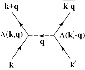
Figure 1: A diagrammatic representation of the interaction (48) in the absence of the Peierls phase factors. The vertex $\Lambda({\mib k},{\mib q})$ is given by eq. (49), and $\overline{{\mib k}\!+\!{\mib q}}$ denotes the wave vector in the first Brillouin zone corresponding to ${\mib k}+{\mib q}$ in the extended zone scheme.

It is also possible to expand eq. (49a) in powers of ${\mib B}$ as

$$\underline{\Lambda}({\mib k},{\mib q},{\mib B})=\underline{\Lambda}^{\!(0)}({\mib k},{\mib q})+\sum_{j=1}^{\infty}\underline{\Lambda}^{\!(j)}({\mib k},{\mib q},{\mib B})\,.$$ (49b)

The expressions of $\underline{\Lambda}^{\!(j)}$ may be obtained with the same procedure as that of deriving eq. (34). The quantity $\underline{\Lambda}^{\!(0)}$ is given by

$$\Lambda_{bb^{\prime}}^{\!(0)}({\mib k},{\mib q})=\langle\vec{u}_{b\overline{{\mib k}+{\mib q}}}|{\rm e}^{i{\mib K}_{{\mib k}+{\mib q}}\cdot{\mib r}}|\vec{u}_{b^{\prime}{\mib k}}\rangle\,,$$ (50a)

with $${\mib K}_{{\mib k}+{\mib q}}\!\equiv\!{\mib k}\!+\!{\mib q}\!-\!\overline{{\mib k}\!+\!{\mib q}} \underline{\Lambda}^{\!(1)}({\mib k},{\mib q})\!=\!\underline{\Lambda}^{\!\prime(1)}({\mib k},{\mib q})+\underline{S}^{(1)}(\overline{{\mib k}\!+\!{\mib q}})\underline{\Lambda}^{(0)}({\mib k},{\mib q})+\underline{\Lambda}^{\!(0)}({\mib k},{\mib q})\underline{S}^{(1)}({\mib k})$$ a reciprocal lattice vector. The first-order term is obtained from together with eqs. (26) and (120a) as

$$\underline{\Lambda}^{\!(1)}({\mib k},{\mib q})=-\frac{1}{2}h_{\alpha\beta}\,\underline{x}^{\alpha}(\overline{{\mib k}\!+\!{\mib q}})\,\nabla_{\!{\mib k}}^{\beta}\underline{\Lambda}^{\!(0)}({\mib k},{\mib q})$$

$$\hskip 14.22636pt-\frac{1}{2}h_{\alpha\beta}\!\left[\nabla_{\!{\mib k}}^{\beta}\underline{\Lambda}^{\!(0)}({\mib k},{\mib q})\right]\underline{x}^{\alpha}({\mib k})\,.$$ (50b)

Note that the argument of $$\underline{x}^{\alpha} {\mib k} \overline{{\mib k}\!+\!{\mib q}} \underline{\Lambda}^{\!(0)}({\mib k},{\mib q}) \underline{x}^{\alpha} \hbar\underline{\tilde{v}}^{\beta}$$ is () when it appears to the right (left) of ; keeping this rule in mind and dropping the argument of , eq. (50b) may be written exactly as the contribution of eq. (34a). This rule also applies to higher-order terms.

The second-order term is calculated similarly. We obtain an expression analogous to the $\hbar\underline{\tilde{\mib v}}$ contributions of eq. (34b) as

$$\underline{\Lambda}^{\!(2)}({\mib k},{\mib q})$$

$$=\frac{1}{2}h_{\alpha\beta}h_{\alpha^{\prime}\beta^{\prime}}\nabla_{\!{\mib k}}^{\beta}\biggl{[}\bigl{\{}\underline{x}^{\alpha}(\overline{{\mib k}\!+\!{\mib q}}),\underline{x}^{\alpha^{\prime}}(\overline{{\mib k}\!+\!{\mib q}})\bigr{\}}\nabla_{\!{\mib k}}^{\beta^{\prime}}\!\underline{\Lambda}^{\!(0)}\!({\mib k},{\mib q})$$

$$\hskip 48.36967pt+\bigl{[}\nabla_{\!{\mib k}}^{\beta^{\prime}}\!\underline{\Lambda}^{\!(0)}\!({\mib k},{\mib q})\bigr{]}\bigl{\{}\underline{x}^{\alpha}({\mib k}),\underline{x}^{\alpha^{\prime}}({\mib k})\bigr{\}}\biggr{]}$$

$$-\frac{1}{4}h_{\alpha\beta}h_{\alpha^{\prime}\beta^{\prime}}\biggl{[}\bigl{\{}\underline{x}^{\alpha}(\overline{{\mib k}\!+\!{\mib q}}),\underline{x}^{\alpha^{\prime}}(\overline{{\mib k}\!+\!{\mib q}})\bigr{\}}\nabla_{\!{\mib k}}^{\beta}\nabla_{\!{\mib k}}^{\beta^{\prime}}\!\underline{\Lambda}^{\!(0)}\!({\mib k},{\mib q})$$

$$\hskip 31.29802pt+\bigl{[}\nabla_{\!{\mib k}}^{\beta}\nabla_{\!{\mib k}}^{\beta^{\prime}}\!\underline{\Lambda}^{\!(0)}\!({\mib k},{\mib q})\bigr{]}\bigl{\{}\underline{x}^{\alpha}({\mib k}),\underline{x}^{\alpha^{\prime}}({\mib k})\bigr{\}}\biggr{]}$$

$$+\frac{i}{4}h_{\alpha\beta}h_{\alpha^{\prime}\beta^{\prime}}\nabla_{\!{\mib k}}^{\beta}\nabla_{\!{\mib k}}^{\beta^{\prime}}\biggl{[}\underline{x}^{\alpha^{\prime}}(\overline{{\mib k}\!+\!{\mib q}})\nabla_{\!{\mib k}}^{\alpha}\!\underline{\Lambda}^{\!(0)}\!({\mib k},{\mib q})$$

$$\hskip 56.9055pt-\nabla_{\!{\mib k}}^{\alpha}\!\underline{\Lambda}^{\!(0)}\!({\mib k},{\mib q})\,\underline{x}^{\alpha^{\prime}}({\mib k})\biggr{]}$$

$$-\frac{1}{2}\left[\underline{\cal O}^{(1)}(\overline{{\mib k}\!+\!{\mib q}})\underline{\Lambda}^{\!(1)}({\mib k},{\mib q})+\underline{\Lambda}^{\!(1)}({\mib k},{\mib q})\underline{\cal O}^{(1)}({\mib k})\right]$$

$$+\frac{1}{8}\left[\underline{\cal O}^{(1)}(\overline{{\mib k}\!+\!{\mib q}})\underline{\cal O}^{(1)}(\overline{{\mib k}\!+\!{\mib q}})\underline{\Lambda}^{\!(0)}({\mib k},{\mib q})\right.$$

$$-2\underline{\cal O}^{(1)}(\overline{{\mib k}\!+\!{\mib q}})\underline{\Lambda}^{\!(0)}({\mib k},{\mib q})\underline{\cal O}^{(1)}({\mib k})$$

$$\left.+\underline{\Lambda}^{\!(0)}({\mib k},{\mib q})\underline{\cal O}^{(1)}({\mib k})\underline{\cal O}^{(1)}({\mib k})\right]$$

$$+\frac{i}{2}h_{\alpha\beta}\nabla_{\!{\mib k}}^{\beta}\left\{\underline{\cal O}^{(1)}(\overline{{\mib k}\!+\!{\mib q}})\nabla_{\!{\mib k}}^{\alpha}\underline{\Lambda}^{\!(0)}({\mib k},{\mib q})\right.$$

$$\hskip 22.76219pt\left.-\left[\nabla_{\!{\mib k}}^{\alpha}\underline{\Lambda}^{\!(0)}({\mib k},{\mib q})\right]\underline{\cal O}^{(1)}({\mib k})\right\}\,.$$ (50c)

3.2 Perturbation expansion

With these preliminaries, we proceed to the calculation of the thermodynamic potential $\Omega\!=\!-T\ln{\rm Tr}\,{\rm e}^{-\hat{\cal H}_{\rm tot}/T}$, the self-energy $\Sigma_{\nu\nu^{\prime}}$ and Green’s function $G_{\nu^{\prime}\nu}$ in the framework of the conserving approximation.[64, 65]

Let us define the Matsubara Green’s function by

$$G_{\nu^{\prime}\nu}(\varepsilon_{n})=-\int_{0}^{1/T}\!\!\!\!\langle\,T_{\tau}\,c_{\nu^{\prime}}(\tau)\,c_{\nu}^{\dagger}\,\rangle\,{\rm e}^{i\varepsilon_{n}\tau}\,{\rm d}\tau\,,$$ (51)

which as ${\cal U}\!\rightarrow\!0$ reduces to $g_{\nu^{\prime}\nu}(\varepsilon_{n})$ of eq. (40). As shown by Luttinger and Ward,[63] $\Omega$ can be written as a functional of $\underline{G}$ as

$$\Omega=-T\sum_{n}{\rm Tr}\bigl{\{}\ln\bigl{[}\underline{\cal H}+\underline{\Sigma}-i\varepsilon_{n}\underline{1}\bigr{]}+\underline{\Sigma}\,\underline{G}\bigr{\}}{\rm e}^{i\varepsilon_{n}0_{+}}+\Phi[\underline{G}]\,.$$ (52)

Here $0_{+}$ is an infinitesimal positive constant and $\Phi$ denotes contributions of all the skeleton diagrams in the bare perturbation expansion for $\Omega$ with $\underline{G}$ used as the propagator. The self-energy is obtained from $\Phi$ by

$$\Sigma_{\nu\nu^{\prime}}(\varepsilon_{n})=\frac{1}{T}\,\frac{\delta\Phi}{\delta G_{\nu^{\prime}\nu}(\varepsilon_{n})}\,.$$ (53a)

With this relation, $$\Omega \underline{G}$$ is stationary with respect to a variation in satisfying Dyson’s equation:

$$\left[i\varepsilon_{n}\underline{1}-\underline{\cal H}-\underline{\Sigma}(\varepsilon_{n})\right]\underline{G}(\varepsilon_{n})=\underline{1}\,.$$ (53b)

The conserving approximation denotes approximating $\Phi$ by some selected diagrams and determining $\underline{G}$ and $\underline{\Sigma}$ self-consistently by eq. (53).[64, 65] Its advantages may be summarized as follows: (i) both the equilibrium and dynamical properties can be described within the same approximation with various conservation laws automatically satisfied; (ii) the Laudau Fermi-liquid corrections,[66, 67] or vertex corrections in a different terminology, are automatically included. For example, the lowest-order conserving approximation is nothing but the Hartree-Fock approximation where $\Phi^{\rm HF}$ and $\Sigma_{\nu\nu^{\prime}}^{\rm HF}$ are given by

$$\Phi^{\rm HF}=\frac{T^{2}}{2}\sum_{n_{1},n_{2}}\sum_{\nu_{1}\nu_{2}\nu_{1}^{\prime}\nu_{2}^{\prime}}{\cal U}_{\nu_{1}\nu_{2};\nu_{1}^{\prime}\nu_{2}^{\prime}}[G_{\nu_{1}^{\prime}\nu_{1}}(\varepsilon_{n_{1}})G_{\nu_{2}^{\prime}\nu_{2}}(\varepsilon_{n_{2}})$$

$$\hskip 4.2679pt-G_{\nu_{1}^{\prime}\nu_{2}}(\varepsilon_{n_{1}})G_{\nu_{2}^{\prime}\nu_{1}}(\varepsilon_{n_{2}})]{\rm e}^{i\varepsilon_{n_{1}}\!0_{+}+i\varepsilon_{n_{2}}\!0_{+}}\,,$$ (54a)

$$\Sigma_{\nu\nu^{\prime}}^{\rm HF}=T\sum_{n_{1}}\sum_{\nu_{1}\nu_{1}^{\prime}}({\cal U}_{\nu\nu_{1};\nu^{\prime}\nu_{1}^{\prime}}\!-{\cal U}_{\nu\nu_{1};\nu_{1}^{\prime}\nu^{\prime}})G_{\nu_{1}^{\prime}\nu_{1}}(\varepsilon_{n_{1}}){\rm e}^{i\varepsilon_{n_{1}}\!0_{+}}\,,$$ (54b)

respectively.

It follows from eqs. (32) and (48) that $\Sigma_{\nu\nu^{\prime}}(\varepsilon_{n})$ and $G_{\nu^{\prime}\nu}(\varepsilon_{n})$ can be expanded as

$$\Sigma_{b{\mib R},b^{\prime}{\mib R}^{\prime}}(\varepsilon_{n})=\frac{{\rm e}^{iI_{{\mib R}{\mib R}^{\prime}}}}{N_{\rm c}}\sum_{{\mib k}}{\rm e}^{i{\mib k}\cdot({\mib R}-{\mib R}^{\prime})}\Sigma_{bb^{\prime}}(\varepsilon_{n},{\mib k})\,,$$ (55a)

$$G_{b^{\prime}{\mib R}^{\prime},b{\mib R}}(\varepsilon_{n})=\frac{{\rm e}^{iI_{{\mib R}^{\prime}{\mib R}}}}{N_{\rm c}}\sum_{{\mib k}}{\rm e}^{i{\mib k}\cdot({\mib R}^{\prime}-{\mib R})}G_{b^{\prime}b}(\varepsilon_{n},{\mib k})\,.$$ (55b)

This is proved by induction as follows: First, the non-interacting Green’s function $g_{\nu^{\prime}\nu}(\varepsilon_{n})$ is already given in the form of eq. (55b) as eq. (41). We next assume the expression (55b) and substitute it into eq. (53a) to calculate $\Sigma_{\nu\nu^{\prime}}(\varepsilon_{n})$ order by order by using eq. (22). We then find that the self-energy can also be written as eq. (55a), i.e., the same expression as the non-interacting Hamiltonian (32). It hence follows that $G_{\nu^{\prime}\nu}(\varepsilon_{n})$ may be written as eq. (55b). This completes the proof.

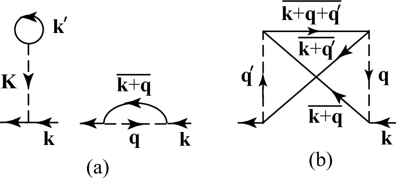
Figure 2: Some typical diagrams for the self-energy: (a) the Hartree and Fock terms; (b) the second-order exchange contribution.

To see how to calculate $\underline{\Sigma}(\varepsilon_{n},{\mib k})$ practically, we present expressions of $\underline{\Sigma}^{\rm HF}({\mib k})$ obtained from eq. (54b), see also Fig. 2(a), and $\underline{\Sigma}^{\rm 2e}(\varepsilon_{n},{\mib k})$ which corresponds to the diagram of Fig. 2(b):

$$\underline{\Sigma}^{\rm HF}({\mib k})$$

$$=\frac{T}{V}\sum_{n}\biggl{[}\sum_{{\mib K}}{\cal U}_{{\mib K}}\underline{\Lambda}({\mib k},{\mib K})\!\sum_{{\mib k}^{\prime}}\!{\rm Tr}\underline{\Lambda}({\mib k}^{\prime},-{\mib K})\underline{G}(\varepsilon_{n},{\mib k}^{\prime})$$

$$-\sum_{{\mib q}}{\cal U}_{{\mib q}}\,\underline{\Lambda}(\overline{{\mib k}\!+\!{\mib q}},-{\mib q})\!\otimes\!\underline{G}(\varepsilon_{n},\overline{{\mib k}\!+\!{\mib q}})\!\otimes\!\underline{\Lambda}({\mib k},{\mib q})\biggr{]}{\rm e}^{i\varepsilon_{n}\!0_{+}}\,,$$

(56a)

$$\underline{\Sigma}^{\rm 2e}(\varepsilon_{n},{\mib k})=\frac{T^{2}}{V^{2}}\!\sum_{n_{1}n_{2}}\sum_{{\mib q}{\mib q}^{\prime}}{\cal U}_{{\mib q}}\,{\cal U}_{{\mib q}^{\prime}}\bigl{[}\,\underline{\Lambda}(\overline{{\mib k}\!+\!{\mib q}^{\prime}},-{\mib q}^{\prime})$$

$$\hskip 28.45274pt\otimes\,\underline{G}(\varepsilon_{n+n_{2}-n_{1}},\overline{{\mib k}\!+\!{\mib q}^{\prime}})\otimes\underline{\Lambda}(\overline{{\mib k}\!+\!{\mib q}\!+\!{\mib q}^{\prime}},-{\mib q})$$

$$\hskip 28.45274pt\otimes\,\underline{G}(\varepsilon_{n_{2}},\overline{{\mib k}\!+\!{\mib q}\!+\!{\mib q}^{\prime}})\otimes\underline{\Lambda}(\overline{{\mib k}\!+\!{\mib q}},{\mib q}^{\prime})$$

$$\hskip 28.45274pt\otimes\,\underline{G}(\varepsilon_{n_{1}},\overline{{\mib k}\!+\!{\mib q}})\otimes\underline{\Lambda}({\mib k},{\mib q})\,\bigr{]}\,,$$ (56b)

where $\otimes$ operates on the ${\mib k}^{\prime}$ or ${\mib k}$ dependences of the adjacent functions. Note that removing the operator $\otimes$ in the above expressions yields the self-energies at ${\mib B}\!=\!{\mib 0}$. We hence have a simple rule to calculate the ${\mib k}$-space self-energy for $B\!>\!0$ using only the zero-field Feynman diagrams as follows: (i) Label each of the connected electron lines with the same wave vector, like ${\mib k}$ or ${\mib k}^{\prime}$ in the above examples, and insert the operator $\otimes$ of eq. (23) between every adjacent $\underline{\Lambda}$ and $\underline{G}$. (ii) We can remove any single operator $\otimes$ within every closed electron loop, as in the first term of eq. (56a), because of the absence of the Peierls phase factor in the final calculation of using eq. (22); this may also be proved directly in ${\mib k}$ space by using eq. (24b). The rules (i) and (ii) apply also to the calculations of $\Omega$ and $\underline{G}(\varepsilon_{n},{\mib k})$.

We now provide ${\mib k}$-space expressions of eqs. (52) and (53). Noting the rule (ii) above, we realize that $\Phi$ in eq. (52) is given alternatively as a functional of $\underline{G}(\varepsilon_{n},{\mib k})$ as

$$\Phi=T\sum_{n}\sum_{\ell=1}^{\infty}\frac{1}{2\ell}\sum_{{\mib k}}{\rm Tr}\,\underline{\Sigma}^{\ell}\!(\varepsilon_{n},{\mib k},{\mib B})\,\underline{G}(\varepsilon_{n},{\mib k},{\mib B}){\rm e}^{i\varepsilon_{n}0_{+}}\,,$$ (57)

with $\underline{\Sigma}^{\ell}$ the contribution of the $\ell$th-order skeleton diagrams to $\underline{\Sigma}$. We hence have

$$\Sigma_{bb^{\prime}}(\varepsilon_{n},{\mib k},{\mib B},\{\underline{G}\})=\frac{1}{T}\,\frac{\delta\Phi}{\delta G_{b^{\prime}b}(\varepsilon_{n},{\mib k},{\mib B})}\,.$$ (58a)

Next, Dyson’s equation of eq. (53b) is transformed into $$\left[i\varepsilon_{n}\underline{1}\!-\!\underline{\cal H}({\mib k},{\mib B})\!-\!\underline{\Sigma}(\varepsilon_{n},{\mib k},{\mib B})\right]\otimes\underline{G}(\varepsilon_{n},{\mib k},{\mib B})\!=\!\underline{1}$$, as shown by using eqs. (32), (55), and (22). It may be written alternatively as

$$\sum_{{\mib k}^{\prime}}\delta_{{\mib k}{\mib k}^{\prime}}\!\left[i\varepsilon_{n}\underline{1}\!-\!\underline{\cal H}({\mib\kappa},{\mib B})\!-\!\underline{\Sigma}(\varepsilon_{n},{\mib\kappa},{\mib B})\right]\underline{G}(\varepsilon_{n},{\mib k}^{\prime},{\mib B})=\underline{1}\,,$$ (58b)

where ${\mib\kappa}$ is defined by eq. (43). Hence the functional (52) is given in ${\mib k}$ space by

$$\Omega=-T\sum_{n}{\rm Tr}\biggl{[}{\rm Tr}_{\mib k}\ln\!\left\{\left[\,\underline{\cal H}({\mib\kappa},{\mib B})\!+\!\underline{\Sigma}(\varepsilon_{n},{\mib\kappa},{\mib B})\!-\!i\varepsilon_{n}\underline{1}\,\right]\right\}$$

$$+\sum_{\mib k}\underline{\Sigma}(\varepsilon_{n},{\mib k},{\mib B})\,\underline{G}(\varepsilon_{n},{\mib k},{\mib B})\biggr{]}\,{\rm e}^{i\varepsilon_{n}0_{+}}+\Phi[\underline{G}]\,,$$ (59)

with Tr${}_{\mib k}$ denoting the trace in ${\mib k}$ space. It satisfies

$$\frac{\delta\Omega}{\delta G_{b^{\prime}b}(\varepsilon_{n},{\mib k},{\mib B})}=0\,,$$ (60)

as shown by using eq. (58).

Finally, eqs. (57) and (58a) may be expanded with respect to the explicit ${\mib B}$ dependences originating from the vertex $\Lambda$ and the operator $\otimes$ as

$$\Phi({\mib B},\{\underline{G}\})=\Phi^{(0)}(\{\underline{G}\})+\sum_{j=1}^{\infty}\Phi^{(j)}({\mib B},\{\underline{G}\})\,,$$ (61)

$$\underline{\Sigma}(\varepsilon_{n},{\mib k},{\mib B},\{\underline{G}\})=\underline{\Sigma}^{(0)}(\varepsilon_{n},{\mib k},\{\underline{G}\})$$

$$\hskip 56.9055pt+\sum_{j=1}^{\infty}\underline{\Sigma}^{(j)}(\varepsilon_{n},{\mib k},{\mib B},\{\underline{G}\})\,,$$ (62)

where $\Phi^{(j)}$ and $\underline{\Sigma}^{(j)}$ are quantities of the order $B^{j}$. Note that $\Phi^{(0)}$ and $\underline{\Sigma}^{(0)}$ are different from those at ${\mib B}\!=\!{\mib 0}$ due to the implicit ${\mib B}$ dependences through $\underline{G}$. It follows from eq. (57) that $\Phi^{(j)}$ is connected with $\underline{\Sigma}^{(j)}$ as

$$\Phi^{(j)}=T\sum_{n\ell}\frac{1}{2\ell}\sum_{{\mib k}}{\rm Tr}\underline{\Sigma}^{\ell(j)}\!(\varepsilon_{n},{\mib k},{\mib B})\underline{G}(\varepsilon_{n},{\mib k},{\mib B})\,{\rm e}^{i\varepsilon_{n}0_{+}}\,.$$ (63)

3.3 Hartree-Fock approximation

We here concentrate on the Hartree-Fock approximation. Since there is no $\varepsilon_{n}$ dependence in the self-energy $\underline{\Sigma}^{{\rm HF}}({\mib k})$, eqs. (57)-(60) can be simplified further by performing every summation over $n$ with the Fermi distribution function $f(\varepsilon)\!\equiv\!1/({\rm e}^{\varepsilon/T}\!+\!1)$.[63] The potentials $\Omega$ and $\Phi$ are thereby transformed into the functionals of the occupation number defined by

$$\underline{n}({\mib k},{\mib B})\equiv T\sum_{n}\underline{G}(\varepsilon_{n},{\mib k},{\mib B})\,{\rm e}^{i\varepsilon_{n}0_{+}}\,.$$ (64)

Indeed, eq. (59) is now approximated (dropping the ${\mib B}$ dependences for simplicity) by

$$\Omega^{{\rm HF}}=-T\,{\rm Tr}\,{\rm Tr}_{{\mib k}}\ln\bigl{\{}\underline{1}+{\rm e}^{-[\underline{\cal H}({\mib\kappa})+\underline{\Sigma}^{{\rm HF}}({\mib\kappa})]/T}\bigr{\}}$$

$$\hskip 7.11317pt-\sum_{{\mib k}}{\rm Tr}\,\underline{n}({\mib k})\,\underline{\Sigma}^{{\rm HF}}\!({\mib k})+\Phi^{{\rm HF}}\,,$$ (65)

with

$$\Phi^{{\rm HF}}$$

$$=\!\frac{1}{2V}\!\left\{\sum_{{\mib k}{\mib k}^{\prime}}\!\sum_{{\mib K}}{\cal U}_{{\mib K}}{\rm Tr}[\,\underline{n}({\mib k})\underline{\Lambda}({\mib k},{\mib K})]\,{\rm Tr}[\,\underline{n}({\mib k}^{\prime})\underline{\Lambda}({\mib k}^{\prime},-{\mib K})]\right.$$

$$-\!\sum_{{\mib k}{\mib q}}{\cal U}_{{\mib q}}{\rm Tr}\underline{\Lambda}(\overline{{\mib k}\!+\!{\mib q}},-{\mib q})\otimes\underline{n}(\overline{{\mib k}\!+\!{\mib q}})\otimes\underline{\Lambda}({\mib k},{\mib q})\otimes\underline{n}({\mib k})\biggr{\}}.$$

(66)

The self-energy $\underline{\Sigma}^{{\rm HF}}\!({\mib k})$ of eq. (56a) is obtained from $\Phi^{{\rm HF}}$ by

$$\Sigma_{bb^{\prime}}^{{\rm HF}}\!({\mib k})=\frac{\delta\Phi^{{\rm HF}}}{\delta n_{b^{\prime}b}({\mib k})}\,.$$ (67a)

It hence follows that $$\Omega^{{\rm HF}} \underline{n}({\mib k})$$ is stationary with respect to a variation in satisfying

$$\underline{n}({\mib k})=\frac{1}{\displaystyle{\rm e}^{[\underline{\cal H}({\mib k})+\underline{\Sigma}^{{\rm HF}}({\mib k})]/T}+\underline{1}}\,.$$ (67b)

Equations (67a) and (67b) constitute a closed set of self-consistent equations.

Finally, $\Phi^{{\rm HF}}$ and $\underline{\Sigma}^{{\rm HF}}$ can be expanded with respect to the explicit ${\mib B}$ dependences as eqs. (61) and (62), respectively. The expressions of $\Phi^{{\rm HF}(j)}$ and $\underline{\Sigma}^{{\rm HF}(j)}$ are given in Appendix B to clarify some of their fundamental properties.

3.4 Density functional theory

Extensive theoretical studies have been carried out for more than three decades to describe atoms and solids quantitatively based on the DFT.[52, 54] It is thereby established now as one of the most efficient and reliable methods for the quantitative understanding of solids. Hence it is well worth applying the present method to the density functional theory.

We consider the cases where the exchange-correlation energy $E_{\rm xc}$ is given as a functional of the spin density:

$$n_{\pm}({\mib r})=T\sum_{n}{\rm Tr}\,\frac{1}{2}(\underline{1}\pm\underline{\tau}_{3})\,\underline{G}({\mib r},{\mib r},\varepsilon_{n})\,{\rm e}^{i\varepsilon_{n}0_{+}}\,,$$ (68)

where $\underline{1}$, $\underline{\tau}_{3}$, and $\underline{G}$ are $2\!\times\!2$ matrices corresponding to the spin degrees of freedom with $\underline{\tau}_{3}$ denoting the third Pauli matrix. Let us expand $\underline{G}({\mib r},{\mib r},\varepsilon_{n})$ in eq. (68) with respect to the basis functions of eq. (7) and transform the resulting expression with the procedures of eqs. (13), (16) and (22). We thereby obtain

$$n_{\pm}({\mib r})=\frac{1}{N_{\rm c}}\sum_{{\mib k}}{\rm Tr}\,\underline{n}({\mib k})\,\underline{\rho}^{\pm}({\mib k},{\mib r})\,,$$ (69)

where $\underline{n}({\mib k})$ is given by eq. (64) and $\underline{\rho}^{\pm}({\mib k},{\mib r})$ is defined by

$$\underline{\rho}^{\pm}({\mib k},{\mib r})\equiv\underline{\cal S}({\mib k})\otimes\underline{\rho}^{\prime\,\pm}({\mib k},{\mib r})\otimes\underline{\cal S}({\mib k})\,,$$ (70)

with

$${\rho}_{bb^{\prime}}^{\prime\,\pm}({\mib k},{\mib r})\equiv\,{\rm e}^{ih_{\alpha\beta}\nabla_{{\mib k}}^{\alpha}\nabla_{{\mib k}^{\prime}}^{\beta}}\!\left.\vec{u}_{b{\mib k}}^{\dagger}({\mib r})\frac{N_{\rm c}}{2}(\underline{1}\pm\underline{\tau}_{3})\vec{u}_{b^{\prime}{\mib k}^{\prime}}({\mib r})\right|_{{\mib k}^{\prime}={\mib k}}.$$ (71)

The factor $N_{\rm c}$ is introduced in eq. (71) to make $\rho_{bb^{\prime}}^{\prime\,\pm}({\mib k},{\mib r})$ finite in the thermodynamic limit. Note that $\underline{\rho}^{\pm}({\mib k},{\mib r})$ in eq. (69) is just a matrix element with no information on the occupation number. It hence follows that the DFT as a functional of $n_{\pm}({\mib r})$ can be written alternatively as a functional of $\underline{n}({\mib k})$.

The thermodynamic potential of the DFT is given in a form similar to eq. (65) of the Hartree-Fock theory as

$$\Omega=-T\,{\rm Tr}\,{\rm Tr}_{{\mib k}}\ln\bigl{\{}\underline{1}+{\rm e}^{-[\underline{\cal H}({\mib\kappa})+\underline{\Sigma}^{{\rm DFT}}({\mib\kappa})]/T}\bigr{\}}$$

$$-\sum_{{\mib k}}{\rm Tr}\,\underline{n}({\mib k})\,\underline{\Sigma}^{{\rm DFT}}\!({\mib k})+\Phi^{\rm DFT}\,.$$ (72)

The quantity $\Phi^{\rm DFT}$ is defined by

$$\Phi^{\rm DFT}=\Phi^{\rm H}[n({\mib r})]+E_{\rm xc}[n_{\sigma}({\mib r})]\,,$$ (73)

where $\Phi^{\rm H}[n({\mib r})]$ and $E_{\rm xc}[n_{\sigma}({\mib r})]$ are the classic Coulomb energy and the exchange-correlation energy, respectively, with $n({\mib r})\!\equiv\!n_{+}({\mib r})+n_{-}({\mib r})$ and $\sigma\!=\!\pm$. The former is given explicitly by

$$\Phi^{\rm H}[n({\mib r})]=\frac{e^{2}}{2}\!\int\!\frac{n({\mib r})n({\mib r}^{\prime})}{|{\mib r}\!-\!{\mib r}^{\prime}|}{\rm d}{\mib r}{\rm d}{\mib r}^{\prime}\,,$$ (74)

which is equivalent to the Hartree term in eq. (66) with $U_{\mib K}\!=\!4\pi e^{2}/K^{2}$; the ${\mib K}\!=\!{\mib 0}$ term should be removed due to the charge neutrality of the system.

The self-energy $\underline{\Sigma}^{{\rm DFT}}({\mib k})$ is obtained from $\Phi^{\rm DFT}$ by

$$\Sigma_{bb^{\prime}}^{{\rm DFT}}({\mib k})=\frac{\delta\Phi^{\rm DFT}}{\delta n_{b^{\prime}b}({\mib k})}\,.$$ (75a)

The condition $$\delta\Omega^{\rm DFT}/\delta n_{b^{\prime}b}({\mib k})\!=\!0$$ for the thermodynamic equilibrium then yields

$$\underline{n}({\mib k})=\frac{1}{{\rm e}^{[\underline{\cal H}({\mib k})+\underline{\Sigma}^{{\rm DFT}}({\mib k})]/T}+\underline{1}}\,,$$ (75b)

which is the Kohn-Sham equation[44] in disguise. Equations (75a) and (75b) should be solved self-consistently for a given $E_{\rm xc}$.

The equivalence between eqs. (59) and (72) for the exact functional $E_{\rm xc}$ can be established by an argument of using the coupling-constant integral. Suppose we change the interaction of eq. (44) as ${\cal U}\!\rightarrow\!\lambda{\cal U}$ and express the corresponding thermodynamic potential as $\Omega^{\lambda}$. The two expressions (59) and (72) satisfy the same differential equation[63, 52] $\partial\Omega^{\lambda}/\partial\lambda\!=\!\langle\hat{\cal H}^{\lambda}_{\rm int}\rangle/\lambda$ and the same initial condition $\Omega^{\lambda=0}\!=\!\Omega_{0}$, where $\langle\hat{\cal H}^{\lambda}_{\rm int}\rangle$ is the thermodynamic average of the interaction in eq. (45) and $\Omega_{0}$ denotes the non-interacting thermodynamic potential. It hence follows that eqs. (59) and (72) are equivalent.

It is also possible to expand $\Phi^{{\rm DFT}}$ and $\Sigma^{{\rm DFT}}$ with respect to the explicit ${\mib B}$ dependences as eqs. (61) and (62), respectively. The expressions of $\Phi^{{\rm DFT}(j)}$ and $\underline{\Sigma}^{{\rm DFT}(j)}$ are given in Appendix C.

4 Susceptibility

We here study the susceptibility $\chi_{\alpha^{\prime}\alpha}$ of ${\mib B}\!\rightarrow\!{\mib 0}$ based on eq. (59). We first establish a general procedure to calculate $\chi_{\alpha^{\prime}\alpha}$ for a given functional $\Phi$. We then specialize to the Hartree-Fock approximation and the density-functional theory to derive explicit expressions of $\chi_{\alpha^{\prime}\alpha}$ within those approximations. Unlike the treatments by Buot[28] and Misra et al. [31] where they jumped directly to the expression $\chi_{\alpha^{\prime}\alpha}\!\equiv\!-\partial^{2}\Omega/\partial B_{\alpha^{\prime}}\partial B_{\alpha}$, our consideration will proceed in two stages by first calculating the magnetization $M_{\alpha}\!=\!-\partial\Omega/\partial B_{\alpha}$ and then performing another differentiation with respect to $B_{\alpha^{\prime}}$. This approach has an advantage that vertex corrections can be incorporated explicitly in the formula.

4.1 Exact expression

To derive a formally exact expression of $\chi_{\alpha^{\prime}\alpha}$, let us start with classifying various ${\mib B}$ dependences of the thermodynamic potential $\Omega$ in Eq. (59) into three groups. The first category is that through ${\mib\kappa}$ in eq. (43). The second category is the explicit ${\mib B}$ dependences in $\underline{\cal H}({\mib k},{\mib B})$ and $\underline{\Sigma}(\varepsilon_{n},{\mib k},{\mib B},\{\underline{G}\})$. Those in $\underline{\Sigma}$ originate from the ${\mib B}$ dependence in the vertex $\Lambda$ of eq. (49) and the operator $\otimes$ of eq. (23); see eq. (56), for example. The third category is the implicit ${\mib B}$ dependence through $\underline{G}$, which is responsible for the Fermi-liquid corrections.[66, 67] When calculating ${\mib M}\!\equiv\!-\partial\Omega/\partial{\mib B}$, however, we need not consider this third category because of eq. (60).

The dependence through ${\mib\kappa}$ needs a special treatment due to the property (24b). As shown in Appendix D, it does not mix with the other categories for ${\mib B}\!\rightarrow\!{\mib 0}$, yielding the Landau-Peierls diamagnetic susceptibility[68, 1] as

$$\chi_{\alpha^{\prime}\alpha}^{\rm LP}=\frac{\epsilon_{\alpha^{\prime}\beta^{\prime}\gamma^{\prime}}\epsilon_{\alpha\beta\gamma}}{6}\!\left(\frac{e}{2\hbar c}\right)^{\!2}T\sum_{n}{\rm e}^{i\varepsilon_{n}0_{+}}\!\sum_{{\mib k}}{\rm Tr}\biggl{\{}\underline{G}^{2}(\varepsilon_{n},{\mib k})$$

$$\hskip 5.69054pt\times[\nabla_{\!{\mib k}}^{\beta^{\prime}}\nabla_{\!{\mib k}}^{\beta}\underline{G}^{-1}(\varepsilon_{n},{\mib k})][\nabla_{\!{\mib k}}^{\gamma^{\prime}}\nabla_{\!{\mib k}}^{\gamma}\underline{G}^{-1}(\varepsilon_{n},{\mib k})]\biggr{\}}\,.$$ (76)

This expression agrees exactly with eq. (4.15) of Buot.[28]

We next consider the second category. Differentiating eq. (59) with respect to the explicit ${\mib B}$ dependences in $\underline{\cal H}({\mib k},{\mib B})$, $\underline{\Sigma}(\varepsilon_{n},{\mib k},{\mib B},\{\underline{G}\})$, and $\Phi({\mib B},\{\underline{G}\})$, we obtain the relevant magnetization as

$$M_{\alpha}^{\prime}=-T\sum_{n}{\rm e}^{i\varepsilon_{n}0_{+}}\sum_{{\mib k}}{\rm Tr}\,\underline{G}(\varepsilon_{n},{\mib k},{\mib B})\frac{\partial\underline{\cal H}({\mib k},{\mib B})}{\partial B_{\alpha}}$$

$$\hskip 2.84526pt-\,\frac{\partial\Phi({\mib B},\{\underline{G}\})}{\partial B_{\alpha}}\,.$$ (77)

We further differentiate eq. (77) with respect to $B_{\alpha^{\prime}}$ and put ${\mib B}\!=\!{\mib 0}$, where we also need to consider the implicit ${\mib B}$ dependence through $\underline{G}$. Using eq. (58a), we obtain

$$\chi_{\alpha^{\prime}\alpha}^{\prime}=-T\sum_{n}{\rm e}^{i\varepsilon_{n}0_{+}}\sum_{{\mib k}}{\rm Tr}\,\underline{G}\,\frac{\partial^{2}\underline{\cal H}^{(2)}}{\partial B_{\alpha^{\prime}}\partial B_{\alpha}}-\,\frac{\partial\Phi^{(2)}}{\partial B_{\alpha^{\prime}}\partial B_{\alpha}}$$

$$-T\sum_{n}{\rm e}^{i\varepsilon_{n}0_{+}}\sum_{{\mib k}}{\rm Tr}\!\left(\!\frac{\partial\underline{\cal H}^{(1)}}{\partial B_{\alpha}}\!+\!\frac{\partial\underline{\Sigma}^{(1)}}{\partial B_{\alpha}}\!\right)\!\frac{d\underline{G}}{dB_{\alpha^{\prime}}}\,,$$ (78)

where $\underline{\cal H}^{(j)}$, $\Phi^{(j)}$, and $\underline{\Sigma}^{(j)}$ $(j\!=\!1,2)$ are quantities of the order $B^{j}$ with respect to the explicit ${\mib B}$ dependences as given by eqs. (34), (61), and (62), respectively. To find an expression for ${d\underline{G}}/{dB_{\alpha^{\prime}}}$ in eq. (78), we differentiate $\underline{G}^{-1}\underline{G}\!=\!\underline{1}$ with respect to $B_{\alpha^{\prime}}$. We thereby obtain a leading-order equation for ${d\underline{G}}/{dB_{\alpha^{\prime}}}$ given in terms of ${d\underline{G}}^{-1}/{dB_{\alpha^{\prime}}}$ as

$$\frac{d\underline{G}}{dB_{\alpha^{\prime}}}=\underline{G}\left(\!\frac{\partial\underline{\cal H}^{(1)}}{\partial B_{\alpha^{\prime}}}+\frac{\partial\underline{\Sigma}^{(1)}}{\partial B_{\alpha^{\prime}}}+\frac{d\underline{\Sigma}^{(0)}}{dB_{\alpha^{\prime}}}\!\right)\underline{G}\,,$$ (79)

with $\underline{G}\!=\!\underline{G}({\mib B}\!=\!{\mib 0})$ on the right-hand side. The last term in the bracket of eq. (79) originates from the implicit ${\mib B}$ dependence though $\underline{G}$, giving rise to the Fermi-liquid (or vertex) corrections.[66, 67] To find an equation for ${d\underline{\Sigma}^{(0)}}/dB_{\alpha^{\prime}}$, we introduce a vertex function as

$$\Gamma_{b_{1}b_{1}^{\prime},b_{2}b_{2}^{\prime}}^{(0)}(1,2)\equiv\frac{N_{\rm c}}{T^{2}}\,\frac{\delta^{2}\Phi^{(0)}}{\delta G_{b_{1}^{\prime}b_{1}}(1)\delta G_{b_{2}^{\prime}b_{2}}(2)}\,,$$ (80)

with $1\!\equiv\!(\varepsilon_{n_{1}},{\mib k}_{1})$. Noting eq. (58a), we then obtain an expression for $d\underline{\Sigma}^{(0)}\!/{dB_{\alpha^{\prime}}}$ in terms of $d\underline{G}/{dB_{\alpha^{\prime}}}$ as

$$\frac{d\Sigma_{b_{1}b_{1}^{\prime}}^{(0)}(1)}{dB_{\alpha^{\prime}}}=\frac{T}{N_{\rm c}}\sum_{b_{2}b_{2}^{\prime}}\sum_{n_{2}{\mib k}_{2}}\Gamma^{(0)}_{b_{1}b_{1}^{\prime},b_{2}b_{2}^{\prime}}(1,2)\frac{dG_{b_{2}^{\prime}b_{2}}(2)}{dB_{\alpha^{\prime}}}\,.$$ (81)

Equations (79) and (81) form a closed set of equations to determine ${d\underline{G}}/{dB_{\alpha^{\prime}}}$. Introducing the matrix $\underline{\cal I}$ by

$${\cal I}_{b_{1}^{\prime}b_{1}1,b_{2}^{\prime}b_{2}2}\!\equiv\!\frac{T}{N_{\rm c}}\sum_{b_{3}b_{3}^{\prime}}G_{b_{1}^{\prime}b_{3}}(1)G_{b_{3}^{\prime}b_{1}}(1)\Gamma^{(0)}_{b_{3}b_{3}^{\prime};b_{2}b_{2}^{\prime}}(1,2)\,,$$ (82)

the coupled equations are solved formally as

$$\frac{dG_{b_{1}^{\prime}b_{1}}(1)}{dB_{\alpha^{\prime}}}=\sum_{b_{2}b_{2}^{\prime}}\sum_{n_{2}{\mib k}_{2}}\left[(\underline{1}-\underline{\cal I})^{-1}\right]_{b_{1}^{\prime}b_{1}1,b_{2}^{\prime}b_{2}2}$$

$$\times\!\left[\underline{G}(2)\!\left(\!\frac{\partial\underline{\cal H}^{(1)}\!({\mib k}_{2})}{\partial B_{\alpha^{\prime}}}\!+\!\frac{\partial\underline{\Sigma}^{(1)}\!(2)}{\partial B_{\alpha^{\prime}}}\!\right)\!\underline{G}(2)\right]_{b_{2}^{\prime}b_{2}}\!,$$ (83)

with $\underline{1}\!\equiv\!(\delta_{b_{1}^{\prime}b_{2}^{\prime}}\delta_{b_{1}b_{2}}\delta_{{\mib k}_{1}{\mib k}_{2}}\delta_{n_{1}n_{2}})$. Substituting eq. (83) into eq. (78), one can check that the symmetry $\chi^{\prime}_{\alpha^{\prime}\alpha}\!=\!\chi^{\prime}_{\alpha\alpha^{\prime}}$ is satisfied as required.

Equation (78) with eqs. (80), (82), and (83) enables us to calculate the relevant susceptibility $\chi^{\prime}_{\alpha^{\prime}\alpha}$ once the functional $\Phi$ is given explicitly. The total susceptibility is then obtained by

$$\chi_{\alpha^{\prime}\alpha}=\chi_{\alpha^{\prime}\alpha}^{\rm LP}+\chi_{\alpha^{\prime}\alpha}^{\prime}\,,$$ (84)

with $\chi_{\alpha^{\prime}\alpha}^{\rm LP}$ given by eq. (76). The factor $(\underline{1}-\underline{\cal I})^{-1}$ in eq. (83) originates from vertex corrections for both the orbital and spin parts, which have been derived naturally in our treatment. It includes the Stoner enhancement factor as the intra-band contribution of the spin part.

4.2 Hartree-Fock approximation

We now specialize to the Hartree-Fock approximation. Due to the absence of $\varepsilon_{n}$ dependence in the self-energy $\underline{\Sigma}^{{\rm HF}}({\mib k})$, every summation over $n$ can be performed[63] by using the Fermi distribution function:

$$f(\varepsilon)\equiv\frac{1}{{\rm e}^{\varepsilon/T}+1}\,.$$ (85)

Thus, it is possible to simplify the expression of $\chi_{\alpha^{\prime}\alpha}$ further.

Let us adopt the representation of diagonalizing the Hartree-Fock energy in zero field as

$${\cal H}_{bb^{\prime}}({\mib k},{\mib B}\!=\!{\mib 0})+\Sigma_{bb^{\prime}}^{{\rm HF}}({\mib k},{\mib B}\!=\!{\mib 0})=\delta_{bb^{\prime}}\xi_{b{\mib k}}\,.$$ (86)

Then the Landau-Peierls susceptibility of eq. (76) is transformed into

$$\chi_{\alpha^{\prime}\alpha}^{{\rm LP-HF}}\!=\!\frac{1}{6}\!\left(\!\frac{e\hbar}{2c}\!\right)^{\!2}\sum_{b{\mib k}}\frac{\partial f(\xi_{b{\mib k}})}{\partial\xi_{b{\mib k}}}\,\frac{\epsilon_{\alpha^{\prime}\beta^{\prime}\gamma^{\prime}}\epsilon_{\alpha\beta\gamma}}{m^{*}_{\beta^{\prime}\beta}(b{\mib k})\,m^{*}_{\gamma^{\prime}\gamma}(b{\mib k})}\,,$$ (87)

with $m^{*}_{\beta^{\prime}\beta}(b{\mib k})\!\equiv\!\hbar^{2}/(\nabla_{\!{\mib k}}^{\beta^{\prime}}\nabla_{\!{\mib k}}^{\beta}\xi_{b{\mib k}})$. Thus, only the states near the Fermi energy are relevant to the Landau-Peierls susceptibility with the effective mass in place of the bare electron mass. However, this simple result no longer holds in those approximations where the self-energy has $\varepsilon_{n}$ dependence. Equation (87) may be regarded as an extension of the Philippas-McClure result for the electron gas[21] to Bloch electrons.

Next, eq. (78) can be written with respect to $\underline{n}({\mib k})$ of eq. (64) as

$$\chi_{\alpha^{\prime}\alpha}^{\prime{\rm HF}}=-\sum_{{\mib k}}{\rm Tr}\,\underline{n}({\mib k})\,\frac{\partial^{2}\underline{\cal H}^{(2)}({\mib k})}{\partial B_{\alpha^{\prime}}\partial B_{\alpha}}-\,\frac{\partial\Phi^{{\rm HF}(2)}}{\partial B_{\alpha^{\prime}}\partial B_{\alpha}}$$

$$-\sum_{{\mib k}}{\rm Tr}\!\left[\frac{\partial\underline{\cal H}^{(1)}({\mib k})}{\partial B_{\alpha}}\!+\!\frac{\partial\underline{\Sigma}^{{\rm HF}(1)}({\mib k})}{\partial B_{\alpha}}\right]\!\frac{d\underline{n}({\mib k})}{dB_{\alpha^{\prime}}}\,.$$ (88)

The quantity ${d\underline{n}}/{dB_{\alpha^{\prime}}}$ is obtained from eq. (79) by adopting the representation (86) and carrying out the summation over $n$. We thereby arrive at the expression:

$$\frac{dn_{b^{\prime}b}({\mib k})}{dB_{\alpha^{\prime}}}=\frac{f(\xi_{b^{\prime}{\mib k}})\!-\!f(\xi_{b{\mib k}})}{\xi_{b^{\prime}{\mib k}}\!-\!\xi_{b{\mib k}}}\!\left[\frac{\partial{\cal H}_{b^{\prime}b}^{(1)}({\mib k})}{\partial B_{\alpha^{\prime}}}+\frac{\partial{\Sigma}_{b^{\prime}b}^{{\rm HF}(1)}({\mib k})}{\partial B_{\alpha^{\prime}}}\right.$$

$$\hskip 71.13188pt\left.+\frac{d\Sigma^{{\rm HF}(0)}_{b^{\prime}b}({\mib k})}{dB_{\alpha^{\prime}}}\right]\,.$$ (89)

To find an expression of ${d\Sigma^{{\rm HF}(0)}_{b^{\prime}b}({\mib k})}/{dB_{\alpha^{\prime}}}$, we introduce a vertex function in terms of eq. (66) as

$$\Gamma^{{\rm HF}(0)}_{b_{1}b_{1}^{\prime},b_{2}b_{2}^{\prime}}({\mib k}_{1},{\mib k}_{2})\equiv N_{\rm c}\frac{\delta^{2}\Phi^{{\rm HF}(0)}}{\delta n_{b_{1}^{\prime}b_{1}}({\mib k}_{1})\delta n_{b_{2}^{\prime}b_{2}}({\mib k}_{2})}$$

$$=\frac{N_{\rm c}}{V}\sum_{\mib K}\!\left[\,{\cal U}_{\mib K}\Lambda_{b_{1}b_{1}^{\prime}}^{\!(0)}({\mib k}_{1},{\mib K})\Lambda_{b_{2}b_{2}^{\prime}}^{\!(0)}({\mib k}_{2},-{\mib K})-{\cal U}_{{\mib k}_{2}-{\mib k}_{1}+{\mib K}}\right.$$

$$\left.\times\Lambda_{b_{1}b_{2}^{\prime}}^{\!(0)}({\mib k}_{2},{\mib k}_{1}\!-\!{\mib k}_{2}\!-\!{\mib K})\Lambda_{b_{2}b_{1}^{\prime}}^{\!(0)}({\mib k}_{1},{\mib k}_{2}\!-\!{\mib k}_{1}\!+\!{\mib K})\right].$$ (90)

Noting eq. (67a), we then obtain

$$\frac{d\Sigma^{{\rm HF}(0)}_{b^{\prime}b}({\mib k})}{dB_{\alpha^{\prime}}}=\frac{1}{N_{\rm c}}\sum_{b_{1}b_{1}^{\prime}{\mib k}_{1}}\Gamma_{b^{\prime}b,b_{1}b_{1}^{\prime}}^{{\rm HF}(0)}({\mib k},{\mib k}_{1})\frac{dn_{b_{1}^{\prime}b_{1}}({\mib k}_{1})}{dB_{\alpha^{\prime}}}\,.$$ (91)

Equations (89) and (91) form a closed set of equations to determine ${d{n}_{b^{\prime}b}({\mib k})}/{dB_{\alpha^{\prime}}}$. Defining the matrix:

$${\cal I}_{b_{1}^{\prime}b_{1}{\mib k}_{1},b_{2}^{\prime}b_{2}{\mib k}_{2}}^{\rm HF}\!\equiv\frac{1}{N_{\rm c}}\frac{f(\xi_{b_{1}^{\prime}{\mib k}_{1}})\!-\!f(\xi_{b_{1}{\mib k}_{1}})}{\xi_{b_{1}^{\prime}{\mib k}_{1}}\!-\!\xi_{b_{1}{\mib k}_{1}}}\Gamma^{{\rm HF}(0)}_{b_{1}^{\prime}b_{1},b_{2}b_{2}^{\prime}}\!({\mib k}_{1},{\mib k}_{2})\,,$$ (92)

the coupled equations are solved formally as

$$\frac{dn_{b^{\prime}b}({\mib k})}{dB_{\alpha^{\prime}}}=\sum_{b_{1}^{\prime}b_{1}{\mib k}_{1}}\left[(\underline{1}-\underline{\cal I}^{\rm HF})^{-1}\right]_{b^{\prime}b{\mib k},b_{1}^{\prime}b_{1}{\mib k}_{1}}$$

$$\times\frac{f(\xi_{b_{1}^{\prime}{\mib k}_{1}})\!-\!f(\xi_{b_{1}{\mib k}_{1}})}{\xi_{b_{1}^{\prime}{\mib k}_{1}}\!-\!\xi_{b_{1}{\mib k}_{1}}}\!\left[\frac{\partial{\cal H}_{b_{1}^{\prime}b_{1}}^{(1)}({\mib k}_{1})}{\partial B_{\alpha^{\prime}}}\!+\!\frac{\partial{\Sigma}_{b_{1}^{\prime}b_{1}}^{{\rm HF}(1)}({\mib k}_{1})}{\partial B_{\alpha^{\prime}}}\right]\!,$$ (93)

with $\underline{1}\!\equiv\!(\delta_{b^{\prime}b_{1}^{\prime}}\delta_{bb_{1}}\delta_{{\mib k}{\mib k}_{1}})$.

Equations (88) and (93) enables us to calculate $\chi^{\prime{\rm HF}}_{\alpha^{\prime}\alpha}$. The total susceptibility is then obtained by

$$\chi^{{\rm HF}}_{\alpha^{\prime}\alpha}=\chi^{{\rm LP-HF}}_{\alpha^{\prime}\alpha}+\chi^{\prime{\rm HF}}_{\alpha^{\prime}\alpha}\,,$$ (94)

with $\chi^{\rm LP-HF}_{\alpha^{\prime}\alpha}$ given by eq. (87).

4.3 Density functional theory

From a practical viewpoint, it is perhaps most useful at present to derive an expression of the magnetic susceptibility within the density functional theory. We hence consider it in most detail. Since the self-energy does not depend on the Matsubara frequency, however, we can exactly follow the procedure of the previous Hartree-Fock treatment.

Table 1: Quantities necessary to calculate the magnetic susceptibility $\chi^{\rm DFT}_{\alpha^{\prime}\alpha}$ of the density functional theory given by eq. (103). Those with underlines are matrices with respect to the band-spin index $b$.

$\vec{u}_{b{\mib k}}({\mib r})$	$\vec{w}_{b{\mib R}}({\mib r})$	$\xi_{b{\mib k}}$	$\underline{v}^{\alpha}({\mib k})$	$m^{*}_{\beta\beta^{\prime}}(b{\mib k})$	$\epsilon_{\alpha\beta\gamma}$
(4)	(5)	(95)	(106a)	(106b)	(15)

$\underline{x}^{\alpha}({\mib k})$	$\underline{\pi}^{\alpha}({\mib k})$	$\underline{\sigma}^{\alpha}({\mib k})$	$\underline{\cal O}^{(\alpha)}$	$\underline{\cal H}^{{\rm DFT}(\alpha)}$	$\underline{\Gamma}^{{\rm DFT}(0)}$
(20)	(30c)	(30d)	(98)	(99)	(96)

$\underline{\cal I}^{{\rm DFT}}$	$\underline{\Lambda}^{(0)}$	$\underline{\rho}^{\pm(0)}$	$\tilde{\Lambda}^{(\alpha)}_{\mib K}$	$\tilde{n}^{(\alpha)}_{\sigma}({\mib r})$	$F^{(2)}_{\sigma\sigma^{\prime}}({\mib r})$
(97)	(50a)	(129a)	(101a)	(101b)	(133b)

Let us adopt the representation of diagonalizing the Kohn-Sham single-particle energy in zero field as

$${\cal H}_{bb^{\prime}}^{(0)}({\mib k})+\Sigma_{bb^{\prime}}^{{\rm H}(0)}({\mib k})+\Sigma_{bb^{\prime}}^{{\rm xc}(0)}({\mib k})=\delta_{bb^{\prime}}\xi_{b{\mib k}}\,,$$ (95)

where ${\cal H}_{bb^{\prime}}^{(0)}$, $\Sigma_{bb^{\prime}}^{{\rm H}(0)}$, and $\Sigma_{bb^{\prime}}^{{\rm xc}(0)}$ are given by eqs. (30a), (122), and (135), respectively, with ${n}_{bb^{\prime}}({\mib k})\!=\!\delta_{bb^{\prime}}f(\xi_{b{\mib k}})$. The vertex function corresponding to eq. (90) is defined in terms of eq. (73) by

$$\Gamma^{{\rm DFT}(0)}_{b_{1}b_{1}^{\prime},b_{2}b_{2}^{\prime}}({\mib k}_{1},{\mib k}_{2})\equiv N_{\rm c}\frac{\delta^{2}\Phi^{{\rm DFT}(0)}}{\delta n_{b_{1}^{\prime}b_{1}}({\mib k}_{1})\delta n_{b_{2}^{\prime}b_{2}}({\mib k}_{2})}$$

$$=\frac{N_{\rm c}}{V}\sum_{{\mib K}\neq{\mib 0}}\Lambda_{b_{1}b_{1}^{\prime}}^{\!(0)}({\mib k}_{1},{\mib K})\frac{4\pi e^{2}}{K^{2}}\Lambda_{b_{2}b_{2}^{\prime}}^{\!(0)}({\mib k}_{2},-{\mib K})$$

$$+\frac{1}{N_{\rm c}}\sum_{\sigma,\sigma^{\prime}=\pm}\int\!\rho_{b_{1}b_{1}^{\prime}}^{\sigma(0)}({\mib k}_{1},{\mib r})F^{(2)}_{\sigma\sigma^{\prime}}({\mib r})\rho^{\sigma^{\prime}(0)}_{b_{2}b_{2}^{\prime}}({\mib k}_{2},{\mib r})\,{\rm d}{\mib r}\,,$$ (96)

with $\rho_{bb^{\prime}}^{\sigma(0)}$ and $F^{(2)}_{\sigma\sigma^{\prime}}$ given by eqs. (129a) and (133b), respectively. We also introduce a matrix:

$${\cal I}_{b_{1}^{\prime}b_{1}{\mib k}_{1},b_{2}^{\prime}b_{2}{\mib k}_{2}}^{\rm DFT}\!\equiv\frac{1}{N_{\rm c}}\frac{f(\xi_{b_{1}^{\prime}{\mib k}_{1}})\!-\!f(\xi_{b_{1}{\mib k}_{1}})}{\xi_{b_{1}^{\prime}{\mib k}_{1}}\!-\!\xi_{b_{1}{\mib k}_{1}}}\Gamma^{{\rm DFT}(0)}_{b_{1}^{\prime}b_{1},b_{2}b_{2}^{\prime}}\!({\mib k}_{1},{\mib k}_{2})\,,$$ (97)

with $f$ the Fermi distribution function of eq. (85).

It is also useful to define a couple of quantities in terms of eqs. (19a), (34a), (125), and (137) as

$$\underline{\cal O}^{(\alpha)}({\mib k})\equiv\frac{\partial\underline{\cal O}^{(1)}({\mib k})}{\partial B_{\alpha}}=i\epsilon_{\alpha\beta\gamma}\frac{e}{2\hbar c}\underline{x}^{\beta}({\mib k})\underline{x}^{\gamma}({\mib k})\,,$$ (98)

$$\underline{\cal H}^{{\rm DFT}(\alpha)}({\mib k})\equiv\frac{\partial}{\partial B_{\alpha}}\!\left[\underline{\cal H}^{(1)}({\mib k})\!+\!\underline{\Sigma}^{{\rm H}(1)}({\mib k})\!+\!\underline{\Sigma}^{{\rm xc}(1)}({\mib k})\right]$$

$$=-\epsilon_{\alpha\beta\gamma}\frac{e}{2\hbar c}\bigl{(}\{\underline{x}^{\beta},\hbar\underline{v}^{\gamma}+\underline{\pi}^{\gamma}\}+\underline{\sigma}^{\beta\gamma}\bigr{)}$$

$$+\frac{N_{\rm c}}{V}\sum_{{\mib K}\neq{\mib 0}}\underline{\Lambda}^{\!(0)}({\mib k},{\mib K})\,\frac{4\pi e^{2}}{K^{2}}\,\tilde{\Lambda}^{(\alpha)}_{-{\mib K}}$$

$$+\frac{1}{N_{\rm c}}\sum_{\sigma,\sigma^{\prime}=\pm}\int\!\underline{\rho}^{\sigma(0)}({\mib k},{\mib r})\,F^{(2)}_{\sigma\sigma^{\prime}}({\mib r})\,\tilde{n}_{\sigma^{\prime}}^{(\alpha)}({\mib r})\,{\rm d}{\mib r}\,.$$ (99)

Here $\underline{v}^{\alpha}$ is the renormalized velocity:

$$v^{\alpha}_{bb^{\prime}}\equiv\delta_{bb^{\prime}}\frac{1}{\hbar}\,\frac{\partial\xi_{b{\mib k}}}{\partial k_{\alpha}}\,,$$ (100)

and $\underline{\Lambda}^{\!(0)}({\mib k},{\mib K})$, $\underline{\rho}^{\pm(0)}({\mib k},{\mib r})$, and $F^{(2)}_{\sigma\sigma^{\prime}}({\mib r})$ are given by eqs. (50a), (129a) and (133b), respectively. The quantities $\tilde{\Lambda}_{\mib K}^{(\alpha)}$ and $\tilde{n}_{\pm}^{(\alpha)}({\mib r})$ are defined by

$$\tilde{\Lambda}_{\mib K}^{(\alpha)}\equiv\frac{1}{N_{\rm c}}\!\sum_{b{\mib k}}f(\xi_{b{\mib k}})\!\left[{\Lambda}^{\prime(\alpha)}_{bb}({\mib k},{\mib K})\right.$$

$$\hskip 2.84526pt\left.-\{\underline{{\cal O}}^{(\alpha)}({\mib k}),\underline{\Lambda}^{\!(0)}({\mib k},{\mib K})\}_{bb}\right]\,,$$ (101a)

$$\tilde{n}_{\pm}^{(\alpha)}({\mib r})\!\equiv\!\frac{1}{N_{\rm c}}\!\sum_{b{\mib k}}f(\xi_{b{\mib k}})\!\left[{\rho}^{\prime\pm(\alpha)}_{bb}({\mib k},{\mib r})\right.$$

$$\hskip 11.38109pt\left.-\{\underline{{\cal O}}^{(\alpha)}({\mib k}),\underline{\rho}^{\pm(0)}({\mib k},{\mib r})\}_{bb}\right],$$ (101b)

with

$$\underline{\Lambda}^{\prime(\alpha)}({\mib k},{\mib K})\equiv i\epsilon_{\alpha\beta\gamma}\frac{e}{2\hbar c}\underline{x}^{\beta}({\mib k})\underline{\Lambda}^{\!(0)}({\mib k},{\mib K})\underline{x}^{\gamma}({\mib k})\,,$$ (102a)

$$\underline{\rho}^{\prime\pm(\alpha)}({\mib k},{\mib r})\equiv i\epsilon_{\alpha\beta\gamma}\frac{e}{2\hbar c}\underline{x}^{\beta}({\mib k})\underline{\rho}^{\pm(0)}({\mib k},{\mib r})\underline{x}^{\gamma}({\mib k})\,.$$ (102b)

Note $\underline{\Lambda}^{\prime(\alpha)}\!=\!\partial\underline{\Lambda}^{\prime(1)}/\partial B_{\alpha}$ and $\underline{\rho}^{\prime\pm(\alpha)}\!=\!\partial\underline{\rho}^{\prime\,\pm(1)}/\partial B_{\alpha}$ with $\underline{\Lambda}^{\prime(1)}$ and $\underline{\rho}^{\prime\,\pm(1)}$ given by eqs. (120a) and (130a), respectively.

With these preliminaries, the susceptibility $\chi_{\alpha^{\prime}\alpha}^{\rm DFT}$ can be calculated easily by eq. (94) with the replacement of the superscript HF$\rightarrow$DFT. It may be written as a sum of three contributions as

$$\chi_{\alpha^{\prime}\alpha}^{{\rm DFT}}=\chi_{\alpha^{\prime}\alpha}^{{\rm LP-DFT}}+\chi_{\alpha^{\prime}\alpha}^{{\rm PvV-DFT}}+\chi_{\alpha^{\prime}\alpha}^{{\rm(2)-DFT}}\,.$$ (103)

The first term denotes the Landau-Peierls diamagnetism corresponding to eq. (87), given explicitly by

$$\chi_{\alpha^{\prime}\alpha}^{{\rm LP-DFT}}\!=\!\frac{1}{6}\!\left(\!\frac{e\hbar}{2c}\!\right)^{\!\!2}\sum_{b{\mib k}}\frac{\partial f(\xi_{b{\mib k}})}{\partial\xi_{b{\mib k}}}\,\frac{\epsilon_{\alpha^{\prime}\beta^{\prime}\gamma^{\prime}}\epsilon_{\alpha\beta\gamma}}{m^{*}_{\beta^{\prime}\beta}(b{\mib k})\,m^{*}_{\gamma^{\prime}\gamma}(b{\mib k})}\,,$$ (104a)

with $$m^{*}_{\beta^{\prime}\beta}(b{\mib k})\!\equiv\!\hbar^{2}/(\nabla_{\!{\mib k}}^{\beta^{\prime}}\nabla_{\!{\mib k}}^{\beta}\xi_{b{\mib k}})$$.

The second term in eq. (103) comes from the last term in eq. (88), i.e., the second-order perturbation with respect to $\underline{\cal H}^{(1)}\!+\!\underline{\Sigma}^{{\rm DFT}(1)}$. Its intra- and inter-band contributions yield the Pauli and van Vleck paramagnetism, respectively. It is calculated as

$$\chi_{\alpha^{\prime}\alpha}^{{\rm PvV-DFT}}=-\sum_{b_{1}b_{1}^{\prime}{\mib k}_{1}}\sum_{b_{2}b_{2}^{\prime}{\mib k}_{2}}{\cal H}^{{\rm DFT}(\alpha^{\prime})}_{b_{1}b_{1}^{\prime}}({\mib k}_{1})$$

$$\times[(\underline{1}-\underline{\cal I}^{\rm DFT})^{-1}]_{b_{1}^{\prime}b_{1}{\mib k}_{1},b_{2}^{\prime}b_{2}{\mib k}_{2}}\frac{f(\xi_{b_{2}^{\prime}{\mib k}_{2}})\!-\!f(\xi_{b_{2}{\mib k}_{2}})}{\xi_{b_{2}^{\prime}{\mib k}_{2}}\!-\!\xi_{b_{2}{\mib k}_{2}}}$$

$$\times{\cal H}^{{\rm DFT}(\alpha)}_{b_{2}^{\prime}b_{2}}({\mib k}_{2})\,,$$ (104b)

where $\underline{\cal I}^{\rm DFT}$ and $\underline{\cal H}^{{\rm DFT}(\alpha)}$ are given by eqs. (97) and (99), respectively, and $[{f(\xi_{b_{2}^{\prime}{\mib k}_{2}})\!-\!f(\xi_{b_{2}{\mib k}_{2}})}]/({\xi_{b_{2}^{\prime}{\mib k}_{2}}\!-\!\xi_{b_{2}{\mib k}_{2}}})$ should be replaced by $\partial f(\xi_{b_{2}{\mib k}_{2}})/\partial\xi_{b_{2}{\mib k}_{2}}$ for $\xi_{b_{2}^{\prime}{\mib k}_{2}}\!=\!\xi_{b_{2}{\mib k}_{2}}$. Thus, the factor $(\underline{1}-\underline{\cal I}^{\rm DFT})^{-1}$ from vertex corrections is explicitly included in our formula.

The third term in eq. (103) is due to the first two terms in eq. (88). It is calculated from eq. (34b), (126), and (136b) as

$$\chi_{\alpha^{\prime}\alpha}^{{\rm(2)-DFT}}\!=\epsilon_{\alpha^{\prime}\beta^{\prime}\gamma^{\prime}}\epsilon_{\alpha\beta\gamma}\frac{e^{2}}{2c^{2}}\!\sum_{b{\mib k}}\biggl{\{}\!\frac{\partial f(\xi_{b{\mib k}})}{\partial\xi_{b{\mib k}}}\biggl{[}\{\underline{x}^{\beta^{\prime}}\!,\underline{x}^{\beta}\}_{bb}\,v_{b}^{\gamma^{\prime}}\!v_{b}^{\gamma}$$

$$+\frac{1}{4\hbar}(\underline{x}^{\beta}\underline{\pi}^{\gamma^{\prime}}\underline{x}^{\beta^{\prime}}\!+\!\underline{x}^{\beta^{\prime}}\underline{\pi}^{\gamma^{\prime}}\underline{x}^{\beta})_{bb}v_{b}^{\gamma}\!+\!\frac{1}{2\hbar}\{\underline{x}^{\beta},\underline{\sigma}^{\beta^{\prime}\gamma^{\prime}}\}_{bb}v_{b}^{\gamma}$$

$$+\frac{1}{4\hbar}(\underline{x}^{\beta^{\prime}}\underline{\pi}^{\gamma}\underline{x}^{\beta}\!+\!\underline{x}^{\beta}\underline{\pi}^{\gamma}\underline{x}^{\beta^{\prime}})_{bb}v_{b}^{\gamma^{\prime}}\!+\!\frac{1}{2\hbar}\{\underline{x}^{\beta^{\prime}},\underline{\sigma}^{\beta\gamma}\}_{bb}v_{b}^{\gamma^{\prime}}\biggr{]}$$

$$-\frac{1}{2m}f(\xi_{b{\mib k}})\{\underline{x}^{\beta^{\prime}},\underline{x}^{\beta}\}_{bb}\biggl{[}\delta_{\gamma^{\prime}\gamma}-\frac{m}{m^{*}_{\gamma^{\prime}\gamma}(b{\mib k})}\biggr{]}\biggr{\}}$$

$$+\sum_{b{\mib k}}f(\xi_{b{\mib k}})\left[\{\underline{\cal O}^{(\alpha)}({\mib k}),\underline{\cal H}^{(\alpha^{\prime})}\!({\mib k})\}_{bb}\right.$$

$$\hskip 46.94704pt\left.+\{\underline{\cal O}^{(\alpha^{\prime})}({\mib k}),\underline{\cal H}^{(\alpha)}\!({\mib k})\}_{bb}\right]$$

$$+\frac{1}{4}\sum_{bb^{\prime}{\mib k}}f(\xi_{b{\mib k}})(\xi_{b^{\prime}{\mib k}}\!-\!\xi_{b{\mib k}})({\cal O}^{(\alpha^{\prime})}_{bb^{\prime}}{\cal O}_{b^{\prime}b}^{(\alpha)}+{\cal O}^{(\alpha)}_{bb^{\prime}}{\cal O}_{b^{\prime}b}^{(\alpha^{\prime})})$$

$$-\frac{N_{\rm c}^{2}}{V}\sum_{{\mib K}\neq{\mib 0}}\tilde{\Lambda}_{\mib K}^{(\alpha^{\prime})}\,\frac{4\pi e^{2}}{K^{2}}\,\tilde{\Lambda}_{-{\mib K}}^{(\alpha)}$$

$$-2\!\!\!\sum_{\sigma,\sigma^{\prime}=\pm}\int\!\tilde{n}_{\sigma}^{(\alpha)}({\mib r})F^{(2)}_{\sigma\sigma^{\prime}}({\mib r})\tilde{n}_{\sigma^{\prime}}^{(\alpha^{\prime})}({\mib r})\,{\rm d}{\mib r}\,.$$ (104c)

Equation (103) with eq. (104) is one of the main results of the paper. It extends the result of Roth[5] to take both the Coulomb and exchange-correlation effects into account with appropriate vertex corrections. Indeed, one can check that $\chi^{\rm DFT}$ reduces in the non-interacting limit to the expression obtained by Roth.[69] The formula enables us to perform non-empirical calculations of the magnetic susceptibility in solids based on the density-functional theory. Table I summarizes the quantities necessary for the calculation of $\chi^{\rm DFT}_{\alpha^{\prime}\alpha}$.

For practical purposes, it may be worth transforming eq. (100) and $m^{*}_{\beta^{\prime}\beta}(b{\mib k})\!\equiv\!\hbar^{2}/(\nabla_{\!{\mib k}}^{\beta^{\prime}}\nabla_{\!{\mib k}}^{\beta}\xi_{b{\mib k}})$ in eq. (104a) into expressions without differentiations with respect to ${\mib k}$. To this end, let us define a transfer integral in terms of eq. (95) as

$$\bar{t}_{b{\mib R}}\equiv\frac{1}{N_{\rm c}}\sum_{\mib k}{\rm e}^{i{\mib k}\cdot{\mib R}}\,\xi_{b{\mib k}}\,.$$ (105)

Then $v_{b}^{\alpha}({\mib k})$ can be calculated by either of the two expressions:

$$v_{b}^{\alpha}({\mib k})=\frac{1}{\hbar}\frac{\partial\xi_{b{\mib k}}}{\partial k_{\alpha}}=\frac{-i}{\hbar}\sum_{\mib R}{\rm e}^{-i{\mib k}\cdot{\mib R}}\,\bar{t}_{b{\mib R}}\,R_{\alpha}\,.$$ (106a)

Also $$1/m^{*}_{\beta^{\prime}\beta}(b{\mib k})$$ is obtained by

$$\frac{1}{m^{*}_{\beta^{\prime}\beta}(b{\mib k})}=\frac{1}{\hbar^{2}}\frac{\partial^{2}\xi_{b{\mib k}}}{\partial k_{\beta}\partial k_{\beta^{\prime}}}=-\frac{1}{\hbar^{2}}\sum_{\mib R}{\rm e}^{-i{\mib k}\cdot{\mib R}}\,\bar{t}_{b{\mib R}}\,R_{\beta}R_{\beta^{\prime}}\,.$$ (106b)

Together with eq. (20), one may perform a calculation of $\chi^{\rm DFT}_{\alpha^{\prime}\alpha}$ without recourse to numerical differentiations in ${\mib k}$ space.

Three comments are in order before closing the section. First, our susceptibility is defined in terms of the mean flux density ${\mib B}$ by $M_{\alpha^{\prime}}\!=\!\chi_{\alpha^{\prime}\alpha}B_{\alpha}$, which is different from the conventional definition $M_{\alpha^{\prime}}\!=\!\chi_{\alpha^{\prime}\alpha}^{H}H_{\alpha}$ of using the external field ${\mib H}$. However, $\chi_{\alpha^{\prime}\alpha}^{H}$ is found easily from the thermodynamic relation ${\mib H}\!=\!{\mib B}\!-\!4\pi{\mib M}/V$. Indeed, $\chi_{\alpha^{\prime}\alpha}^{H}$ in the crystallographic coordinates is given by

$$\chi_{\alpha^{\prime}\alpha}^{H}=\delta_{\alpha^{\prime}\alpha}\frac{\chi_{\alpha\alpha}}{1-4\pi\chi_{\alpha\alpha}/V}\,.$$ (107)

However, the difference between $\chi_{\alpha\alpha}$ and $\chi_{\alpha\alpha}^{H}$ is negligible for most of the non-magnetic materials. It is also worth noting that choosing ${\mib B}$ as an independent variable is more favorable when extending the theory to superconductors.[70, 71] Secondly, an expression of the spin susceptibility within the density functional theory was already derived by Vosko and Perdew[24] incorporating vertex corrections, which has been a basis of the number of theoretical works on the spin susceptibility of metals.[25, 26, 29] Compared with it, however, the present formula has a couple of advantages that (i) the orbital contribution can be calculated on an equal footing with the spin part and (ii) vertex corrections are incorporated explicitly in the formula without any further approximations. Third, any calculations of the orbital susceptibility based on a model Hamiltonian, such as the Hubbard model, completely fail to incorporate the orbital contributions to $\chi^{\rm PvV}_{\alpha^{\prime}\alpha}$ and $\chi^{(2)}_{\alpha^{\prime}\alpha}$. This is because the key quantity $\underline{x}^{\alpha}({\mib k})$, which originates from the change of the basis functions by the magnetic field, is necessarily set equal to zero in those calculations. Thus, we need to include the field effect on the basis functions for any practical calculations of the orbital magnetism.

5 De Haas-Van Alphen Oscillation

We finally study many-body effects on the dHvA oscillation in metals, limiting our consideration to clean systems without impurity scatterings. A definite advantage here over the previous studies[38, 39, 40, 41] is that the structure of the thermodynamic potential is known explicitly as eq. (59).

Following the original work by Luttinger and Ward,[63] let us regard eq. (59) as a functional of $\underline{\Sigma}(\varepsilon_{n},{\mib k})$ instead of $\underline{G}(\varepsilon_{n},{\mib k})$. It is also stationary with respect to a variation in $\underline{\Sigma}$ satisfying Dyson’s equation (58b). We then write $\underline{\Sigma}$ as a sum of the monotonic and oscillatory parts as

$$\underline{\Sigma}=\underline{\Sigma}^{0}+\underline{\Sigma}^{\rm osc}\,.$$ (108)

As shown by Luttinger within the Hartree-Fock approximation[38] and discussed more generally by Bychkov and Go’kov,[39] the oscillatory part $\underline{\Sigma}^{\rm osc}$ for the spherical Fermi surface is smaller than the monotonic part $\underline{\Sigma}^{0}$ by the order $(\hbar\omega_{\rm c}/\mu)^{3/2}$ ($\omega_{\rm c}$: the cyclotron frequency). We assume that the statement holds up to the infinite order, as expected for three-dimentional Fermi surfaces. Let us expand $\Omega(\underline{\Sigma})$ at $\underline{\Sigma}\!=\!\underline{\Sigma}^{0}$ as

$$\Omega(\underline{\Sigma})=\Omega(\underline{\Sigma}^{0})+\frac{1}{2}\!\!\left.\sum_{b_{1}b_{1}^{\prime}b_{2}b_{2}^{\prime}}\sum_{{\mib k}_{1}{\mib k}_{2}}\!\frac{\delta^{2}\Omega}{\delta\Sigma_{b_{1}b_{1}^{\prime}}({\mib k}_{1})\delta\Sigma_{b_{2}b_{2}^{\prime}}({\mib k}_{2})}\right|_{0}$$

$$\hskip 9.95845pt\times\Sigma_{b_{1}b_{1}^{\prime}}^{\rm osc}({\mib k}_{1})\Sigma_{b_{2}b_{2}^{\prime}}^{\rm osc}({\mib k}_{2})+\cdots\,,$$ (109)

where the term linear in $\underline{\Sigma}^{\rm osc}$ vanishes due to Dyson’s equation (58b) for $\underline{\Sigma}\!=\!\underline{\Sigma}^{0}$ and $\underline{G}\!=\!\underline{G}^{0}$. The second term on the right-hand side of eq. (109) is of the order $(\hbar\omega_{\rm c}/\mu)^{3}$. On the other hand, the first term also has an oscillatory contribution originating from the operator ${\mib\kappa}$ in the logarithm of eq. (59); it is of the order $(\hbar\omega_{\rm c}/\mu)^{5/2}$ relative to the nomotonic part of $\Omega$, as seen from the result of non-interacting systems.[37] It hence follows that we may neglect the second contribution in eq. (109).

The term relevant to the dHvA oscillation in $\Omega(\underline{\Sigma}^{0})$ is given by

$$\Omega^{\rm osc}=-T\!\sum_{n}{\rm Tr}\,{\rm Tr}_{\mib k}\ln\bigl{[}\underline{\cal H}({\mib\kappa},{\mib B})\!+\!\underline{\Sigma}^{0}(\varepsilon_{n},{\mib\kappa},{\mib B})\!-\!i\varepsilon_{n}\underline{1}\bigr{]}$$

$$\hskip 17.07164pt\times{\rm e}^{i\varepsilon_{n}0_{+}}$$

$$=-{\rm Tr}\,{\rm Tr}_{\mib k}\!\int_{-\infty}^{\infty}\!f(\varepsilon)\,\bigl{\{}\ln\bigl{[}\underline{\cal H}({\mib\kappa},{\mib B})\!+\!\underline{\Sigma}^{0{\rm A}}(\varepsilon,{\mib\kappa},{\mib B})\!-\!\varepsilon\underline{1}\bigr{]}$$

$$-\ln\bigl{[}\underline{\cal H}({\mib\kappa},{\mib B})\!+\!\underline{\Sigma}^{0{\rm A}*}(\varepsilon,{\mib\kappa},{\mib B})\!-\!\varepsilon\underline{1}\bigr{]}\bigr{\}}\frac{{\rm d}\varepsilon}{2\pi i}\,,$$ (110)

where $\underline{\Sigma}^{0{\rm A}}(\varepsilon,{\mib\kappa},{\mib B})\!\equiv\!\underline{\Sigma}^{0}(\varepsilon_{n}\!\rightarrow\!-i\varepsilon\!-0_{+},{\mib\kappa},{\mib B})$, and we have used eq. (85) to transform the summation over $n$ into an integration on the real energy axis. Since the oscillation is due to the states near the Fermi level, we only need to consider the region $\varepsilon\!\sim\!0$ in the integral where ${\rm Im}\underline{\Sigma}^{0{\rm A}}(\varepsilon)$ is infinitesimal positive definite and may be approximated by ${0}_{+}\underline{1}$. The double trace in eq. (110) is thereby simplified into

$$\Omega^{\rm osc}=-\sum_{b}{\rm Tr}_{\mib k}\!\int_{-\infty}^{\infty}\!f(\varepsilon)\,\bigl{\{}\ln\bigl{[}h_{b}(\varepsilon,{\mib\kappa},{\mib B})\!-\!\mu\!-\!\varepsilon+i0_{+}\bigr{]}$$

$$\hskip 5.69054pt-\ln\bigl{[}h_{b}(\varepsilon,{\mib\kappa},{\mib B})\!-\!\mu\!-\!\varepsilon-i0_{+}\bigr{]}\bigr{\}}\frac{{\rm d}\varepsilon}{2\pi i}\,,$$ (111)

where $h_{b}(\varepsilon,{\mib k},{\mib B})$ denotes a characteristic value of the Hermitian matrix $\underline{\cal H}({\mib k},{\mib B})\!+\!{\rm Re}\underline{\Sigma}^{0{\rm A}}(\varepsilon,{\mib k},{\mib B})\!+\!\mu\underline{1}$.

Next, we diagonalize $h_{b}(\varepsilon,{\mib\kappa},{\mib B})$ by solving the eigenvalue problem:

$$h_{b}(\varepsilon,{\mib\kappa},{\mib B})\varphi_{\lambda}(\varepsilon,{\mib k},{\mib B})=g_{\lambda}(\varepsilon,{\mib B})\varphi_{\lambda}(\varepsilon,{\mib k},{\mib B})\,,$$ (112a)

where $$\varphi_{\lambda} g_{\lambda} \lambda b N k_{z} {\mib B}\!\parallel\!{\mib z} E_{\lambda}\!=\!E_{\lambda}({\mib B})$$ is an eigenfunction and is its eigenvalue. The subscript is composed of the band-spin index , the Landau level together with an additional quantum number distinguishing its degeneracy, and the wave vector parallel to the magnetic field . We then define the energy as the solution of the equation:

$$E_{\lambda}=g_{\lambda}(E_{\lambda}\!-\!\mu,{\mib B})\,.$$ (112b)

Note that the quantity $1\!-\!\left.\frac{\partial g_{\lambda}}{\partial\varepsilon}\right|_{\varepsilon=0}$ for the state $E_{\lambda}\!=\!\mu$ is inverse of the discontinuity in the single-particle occupation at the Fermi level so that it is positive.[72] It hence follows that $\varepsilon-g_{\lambda}(\varepsilon)+\mu$ is a monotonically increasing function for $\varepsilon\!\sim\!0$ and $E_{\lambda}\!\sim\!\mu$. Equation (111) is thereby transformed into

$$\Omega^{\rm osc}=-\sum_{\lambda}\!\int_{-\infty}^{\infty}\!f(\varepsilon)\,\theta(\varepsilon+\mu-g_{\lambda}(\varepsilon))\,{\rm d}\varepsilon\,,$$

$$=-T\sum_{\lambda}\ln\bigl{[}1+{\rm e}^{-(E_{\lambda}-\mu)/T}\bigr{]}\,,$$ (113)

where $\theta$ is the step function. Equation (113) includes the main oscillatory part of the thermodynamic potential.

Since $E_{\lambda}\!\sim\!\mu$ for the oscillatory part of eq. (113), $E_{\lambda}$ may be calculated accurately by a two-step semiclassical quantization scheme as follows. We first determine the energy $E_{b{\mib k}}\!=\!E_{b{\mib k}}({\mib B})$ by solving

$$E_{b{\mib k}}=h_{b}(E_{b{\mib k}}\!-\!\mu,{\mib k},{\mib B})\,.$$ (114)

We then adopt the Onsager-Lifshitz-Kosevich procedure:[36, 37]

$$S(E_{\lambda})=2\pi(N\!+\!\gamma)\frac{|e|B}{c}\,,$$ (115)

with $N$ an integer, $\gamma$ a constant of the order $1$, and $S(E_{\lambda})$ denoting the area in ${\mib k}^{\prime}$ space perpendicular to ${\mib B}$ specified by $E_{b{\mib k}^{\prime}}\!\leq\!E_{\lambda}$ and $k^{\prime}_{z}\!=\!k_{z}$. Let us substitute those quantized energy levels into eq. (113) and follow the procedure of Lifshitz and Kosevich.[37] We thereby obtain a theory of the dHvA oscillation where the Fermi surface by $E_{b{\mib k}}({\mib B})$ replaces the non-interacting Fermi surface of Lifshitz and Kosevich.[37]

There may be an alternative way to calculate $E_{\lambda}$ semiclassically. We first determine the eigenvalue $g_{\lambda}(\varepsilon,{\mib B})$ in eq. (112a) as a function of $\varepsilon$ by

$$S(\varepsilon,g_{\lambda})=2\pi(N\!+\!\gamma)\frac{|e|B}{c}\,,$$ (116)

where $S(\varepsilon,g_{\lambda})$ denotes the area in ${\mib k}^{\prime}$ space perpendicular to ${\mib B}\!\parallel\!{\mib z}$ specified by $h_{b}(\varepsilon,{\mib k}^{\prime},{\mib B})\!\leq\!g_{\lambda}(\varepsilon,{\mib B})$ and $k^{\prime}_{z}\!=\!k_{z}$. We then obtain the quasiparticle energy $E_{\lambda}$ by solving eq. (112b). Since the characteristic energy of ${\mib\kappa}$ is $\hbar\omega_{\rm c}$, however, the Fermi-surface structures determined by this latter procedure will not differ substantially from those of the first one. It hence follows that we may adopt the first procedure which is certainly more convenient.

Three comments are in order before closing the section. First, the operator ${\mib\kappa}$ appears naturally in the argument of $\underline{\Sigma}^{0}$ as well as in $\underline{\cal H}$ of eq. (110). This fact shows unambiguously the necessity of considering the self-energy to make up the quantized energy levels. Equation (110) thus removes the confusion on the many-body effects of the dHvA oscillation mentioned in Introduction; it supports Luttinger’s original argument, refuting the quantization procedure without the self-energy.[40, 41] Second, the present theory can also treat changes of the energy band structure with ${\mib B}$ by incorporating the explicit ${\mib B}$ dependences in $\underline{\cal H}$ and $\underline{\Sigma}$. Indeed, $\underline{\cal H}({\mib k},{\mib B})$ can be calculated by eq. (34), and $\underline{\Sigma}(\varepsilon_{n},{\mib k},{\mib B})$ may be obtained by the procedure of §3.2 with dropping the oscillatory contribution of $\underline{G}(\varepsilon_{n},{\mib k},{\mib B})$. This effect was neglected by Luttinger[38] but can have a substantial importance, particularly when approaching the magnetic breakdown.[73] It should be noted that this magnetic breakdown is beyond the description of the semiclassical quantization procedure and we have to solve eq. (112) exactly by taking the relevant multiple bands into account. Third, we have used in eq. (111) a characteristic value $h_{b}(\varepsilon,{\mib k},{\mib B})$ and replaced ${\mib k}$ by the operator ${\mib\kappa}$. This procedure is well defined for a simple band where $h_{b}(\varepsilon,{\mib k},{\mib B})$ is analytic in ${\mib k}$.[9] For a complex band with band crossings, however, $h_{b}(\varepsilon,{\mib k},{\mib B})$ may not be analytic in ${\mib k}$ so that the use of $h_{b}(\varepsilon,{\mib\kappa},{\mib B})$ may fail to describe some important effects such as band mixings due to ${\mib\kappa}$. In this situation, one may be required to use a representation where $\underline{\cal H}({\mib k},{\mib B})\!+\!{\rm Re}\underline{\Sigma}^{0{\rm A}}(\varepsilon,{\mib k},{\mib B})\!+\!\mu\underline{1}$ is analytic in ${\mib k}$ and directly solve the eigenvalue problem for $\underline{\cal H}({\mib\kappa},{\mib B})\!+\!{\rm Re}\underline{\Sigma}^{0{\rm A}}(\varepsilon,{\mib\kappa},{\mib B})\!+\!\mu\underline{1}$.

6 Summary

We have constructed a many-body perturbation theory for Bloch electrons in a magnetic field on the basis of the energy band structure in zero field. We have thereby clarified the structures of the thermodynamic potential and the self-energy in a finite magnetic field, and provided a microscopic foundation for the replacement procedure on the self-energy: $\Sigma^{(0)}(\varepsilon_{n},{\mib k})\!\rightarrow\!\Sigma\!\left(\varepsilon_{n},-i{\mib\nabla}\!-\!\frac{e}{\hbar c}{\mib A}\right)$. This perturbation theory is then applied to obtain explicit expressions of the magnetic susceptibility $\chi$ at various approximation levels on the interaction. The result for the density functional theory is given by eq. (103) together with eq. (104) and Table I. It incorporates vertex corrections as well as interband transitions and core polarizations. The expression enables us non-empirical calculations of $\chi$. Thus, it will be useful to improve our quantitative understanding of the magnetic susceptibility in solids. Finally, we have presented a many-body theory on the dHvA oscillation in metals to show unambiguously that the Fermi surface structure with interaction effects in zero field are indeed relevant to the phenomenon.

The present formulation may be extended easily to a non-uniform magnetic field. Hence an application to superconductors will be fairly straightforward. It is also desired to make up a many-body theory on the transport phenomena of Bloch electrons in a magnetic field.

Appendix A Derivation of eq. (48)

We here transform eq. (46) into eq. (48). To start with, let us consider eq. (47) and rewrite $\vec{w}_{\nu_{3}}^{\prime\dagger}({\mib r})\vec{w}_{\nu_{3}^{\prime}}^{\prime}({\mib r})$ in the integral with the procedure of eqs. (13) and (16) as

$$\vec{w}_{\nu_{3}}^{\prime\dagger}({\mib r})\vec{w}_{\nu_{3}^{\prime}}^{\prime}({\mib r})=\frac{{\rm e}^{iI_{{\mib R}_{3}{\mib R}_{3}^{\prime}}}}{N_{\rm c}}\sum_{{\mib k}_{3}{\mib k}_{3}^{\prime}}{\rm e}^{-i{\mib k}_{3}\cdot({\mib r}-{\mib R}_{3})+i{\mib k}_{3}^{\prime}\cdot({\mib r}-{\mib R}_{3}^{\prime})}$$

$$\hskip 51.21495pt\times{\rm e}^{ih_{\alpha\beta}{\mib\nabla}_{\!{\mib k}_{3}}^{\alpha}{\mib\nabla}_{\!{\mib k}_{3}^{\prime}}^{\beta}}\,\vec{u}_{b_{3}{\mib k}_{3}}^{\dagger}({\mib r})\vec{u}_{b_{3}^{\prime}{\mib k}_{3}^{\prime}}({\mib r})\,.$$

The quantity $\vec{w}_{\nu_{4}}^{\prime\dagger}({\mib r}^{\prime})\vec{w}_{\nu_{4}^{\prime}}^{\prime}({\mib r}^{\prime})$ may be expressed similarly. Equation (47) is thereby transformed into

$${\cal U}_{\nu_{3}\nu_{4};\nu_{3}^{\prime}\nu_{4}^{\prime}}^{\prime}$$

$$=\frac{{\rm e}^{iI_{{\mib R}_{3}{\mib R}_{3}^{\prime}}+iI_{{\mib R}_{4}{\mib R}_{4}^{\prime}}}}{N_{\rm c}^{2}V}\sum_{{\mib k}_{3}{\mib k}_{4}{\mib k}_{3}^{\prime}{\mib k}_{4}^{\prime}}{\rm e}^{i{\mib k}_{3}\cdot{\mib R}_{3}-i{\mib k}_{3}^{\prime}\cdot{\mib R}_{3}^{\prime}+i{\mib k}_{4}\cdot{\mib R}_{4}-i{\mib k}_{4}^{\prime}\cdot{\mib R}_{4}^{\prime}}$$

$$\times\!\sum_{\mib q}{\cal U}_{{\mib q}}\,\bar{\Lambda}_{b_{3}b_{3}^{\prime}}^{\prime}({\mib k}_{3},{\mib k}_{3}^{\prime},{\mib q})\bar{\Lambda}_{b_{4}b_{4}^{\prime}}^{\prime}({\mib k}_{4},{\mib k}_{4}^{\prime},-{\mib q})\,,$$ (117)

where $\bar{\Lambda}_{bb^{\prime}}^{\prime}({\mib k},{\mib k}^{\prime},{\mib q})$ is defined by

$$\bar{\Lambda}_{bb^{\prime}}^{\prime}({\mib k},{\mib k}^{\prime},{\mib q})\equiv\!\int{\rm e}^{i(-{\mib k}+{\mib k}^{\prime}+{\mib q})\cdot{\mib r}}\,{\rm e}^{ih_{\alpha\beta}{\mib\nabla}_{\!{\mib k}}^{\alpha}{\mib\nabla}_{\!{\mib k}^{\prime}}^{\beta}}\,\vec{u}_{b{\mib k}}^{\dagger}({\mib r})$$

$$\hskip 48.36967pt\times\vec{u}_{b^{\prime}{\mib k}^{\prime}}({\mib r})\,{\rm d}{\mib r}\,.$$

Note $\bar{\Lambda}_{bb^{\prime}}^{\prime}({\mib k},{\mib k}^{\prime},{\mib q})\!\propto\!\delta_{-{\mib k}+{\mib k}^{\prime}+{\mib q},{\mib K}}$ with ${\mib K}$ a reciprocal lattice vector. It hence follows that ${\mib k}$ in $\bar{\Lambda}_{bb^{\prime}}^{\prime}({\mib k},{\mib k}^{\prime},{\mib q})$ can be written alternatively as ${\mib k}\!=\!\overline{{\mib k}^{\prime}\!+\!{\mib q}}$ with $\overline{{\mib k}^{\prime}\!+\!{\mib q}}$ denoting the wave vector in the first Brillouin zone corresponding to ${\mib k}^{\prime}\!+\!{\mib q}$ in the extended zone scheme. Using this notation and noting ${\rm e}^{i(\overline{{\mib k}^{\prime}+{\mib q}})\cdot{\mib R}}\!=\!{\rm e}^{i({\mib k}^{\prime}+{\mib q})\cdot{\mib R}}$, eq. (117) is simplified into

$${\cal U}_{\nu_{3}\nu_{4};\nu_{3}^{\prime}\nu_{4}^{\prime}}^{\prime}=\frac{{\rm e}^{iI_{{\mib R}_{3}{\mib R}_{3}^{\prime}}+iI_{{\mib R}_{4}{\mib R}_{4}^{\prime}}}}{N_{\rm c}^{2}V}\!\sum_{{\mib k}{\mib k}^{\prime}}\!{\rm e}^{i{\mib k}\cdot({\mib R}_{3}-{\mib R}_{3}^{\prime})+i{\mib k}^{\prime}\cdot({\mib R}_{4}-{\mib R}_{4}^{\prime})}$$

$$\hskip 25.60747pt\times\!\sum_{{\mib q}}{\rm e}^{i{\mib q}\cdot({\mib R}_{3}-{\mib R}_{4})}\,{\cal U}_{{\mib q}}\,\Lambda_{b_{3}b_{3}^{\prime}}^{\prime}({\mib k},{\mib q},{\mib B})$$

$$\hskip 25.60747pt\times\Lambda_{b_{4}b_{4}^{\prime}}^{\prime}({\mib k}^{\prime},-{\mib q},{\mib B})\,,$$ (118)

where $\Lambda_{bb^{\prime}}^{\prime}({\mib k},{\mib q},{\mib B})$ is defined by

$$\Lambda_{bb^{\prime}}^{\prime}({\mib k},{\mib q},{\mib B})$$

$$\equiv\!\int\!{\rm e}^{i{\mib K}_{{\mib k}+{\mib q}}\cdot{\mib r}}\,{\rm e}^{ih_{\alpha\beta}{\mib\nabla}_{\!{\mib k}^{\prime}}^{\alpha}{\mib\nabla}_{\!{\mib k}}^{\beta}}\vec{u}_{b{\mib k}^{\prime}}^{\dagger}({\mib r})\vec{u}_{b^{\prime}{\mib k}}({\mib r})\bigr{|}_{{\mib k}^{\prime}=\overline{{\mib k}+{\mib q}}}\,\,{\rm d}{\mib r}$$

$$=\!\int\!{\rm e}^{ih_{\alpha\beta}{\mib\nabla}_{\!{\mib k}^{\prime}}^{\alpha}{\mib\nabla}_{\!{\mib k}}^{\beta}}\vec{u}_{b{\mib k}^{\prime}}^{\dagger}({\mib r})\,{\rm e}^{i{\mib K}_{{\mib k}+{\mib q}}\cdot{\mib r}}\,\vec{u}_{b^{\prime}{\mib k}}({\mib r})\bigr{|}_{{\mib k}^{\prime}=\overline{{\mib k}+{\mib q}}}\,\,{\rm d}{\mib r}\,,$$

(119a)

with $${\mib K}_{{\mib k}+{\mib q}}\!\equiv\!{\mib k}\!+\!{\mib q}\!-\!\overline{{\mib k}\!+\!{\mib q}} {\mib K}_{{\mib k}+{\mib q}} {\mib k} {\mib k}\!+\!{\mib q} {\mib k} \underline{\Lambda}^{\prime}({\mib k},{\mib q},{\mib B}) {\mib q} \overline{{\mib k}\!+\!{\mib q}}$$. The third line follows from the fact that the discrete reciprocal vector is independent of the infinitesimal changes in or . The wave vector in belongs to the incoming electron, is an additional wave vector from the interaction, and specifies the outgoing electron.

Equation (119a) can be expanded in powers of ${\mib B}$ as

$$\Lambda_{bb^{\prime}}^{\prime}({\mib k},{\mib q},{\mib B})\!=\Lambda_{bb^{\prime}}^{\!(0)}({\mib k},{\mib q})+\sum_{j=1}^{\infty}\Lambda_{bb^{\prime}}^{\!\prime(j)}({\mib k},{\mib q},{\mib B})\,,$$ (119b)

with $\Lambda_{bb^{\prime}}^{\!(0)}$ given by eq. (50a). The quantities $\Lambda_{bb^{\prime}}^{\!\prime(j)}$ can be calculated with the same procedure as that for obtaining eqs. (31a) and (31b). To start with, let us rewrite

$${\rm e}^{i{\mib K}_{{\mib k}+{\mib q}}\cdot{\mib r}}\,|\vec{u}_{b^{\prime}{\mib k}}\rangle=\sum_{b^{\prime\prime}}|\vec{u}_{b^{\prime\prime}\overline{{\mib k}+{\mib q}}}\rangle\Lambda_{b^{\prime\prime}b^{\prime}}^{\!(0)}({\mib k},{\mib q})\,,$$

or equivalently,

$$\langle\vec{u}_{b\overline{{\mib k}+{\mib q}}}|\,{\rm e}^{i{\mib K}_{{\mib k}+{\mib q}}\cdot{\mib r}}=\sum_{b^{\prime\prime}}\Lambda_{bb^{\prime\prime}}^{\!(0)}({\mib k},{\mib q})\langle\vec{u}_{b^{\prime\prime}{\mib k}}|\,,$$

where use has been made of the completeness $$1\!=\!\sum_{b^{\prime\prime}}|\vec{u}_{b^{\prime\prime}\overline{{\mib k}+{\mib q}}}\rangle\langle\vec{u}_{b^{\prime\prime}\overline{{\mib k}+{\mib q}}}|=\sum_{b^{\prime\prime}}|\vec{u}_{b^{\prime\prime}{\mib k}}\rangle\langle\vec{u}_{b^{\prime\prime}{\mib k}}| {\mib B} \underline{\Lambda}^{\!(j)}({\mib k},{\mib q})$$ over the unit cell. We then substitute the above identities into eq. (119a), expand it in powers of to obtain , and average the resulting two different expressions. We thereby obtain the first-order term as

$$\underline{\Lambda}^{\!\prime(1)}({\mib k},{\mib q})=\frac{1}{2}\biggl{\{}\underline{{\cal O}}^{(1)}(\overline{{\mib k}\!+\!{\mib q}})\underline{\Lambda}^{\!(0)}({\mib k},{\mib q})+\underline{\Lambda}^{\!(0)}({\mib k},{\mib q})\underline{\cal O}^{(1)}({\mib k})$$

$$\hskip 48.36967pt-h_{\alpha\beta}\,\underline{x}^{\alpha}(\overline{{\mib k}\!+\!{\mib q}})\,\nabla_{\!{\mib k}}^{\beta}\underline{\Lambda}^{\!(0)}({\mib k},{\mib q})$$

$$\hskip 48.36967pt-h_{\alpha\beta}\!\left[\nabla_{\!{\mib k}}^{\beta}\underline{\Lambda}^{\!(0)}({\mib k},{\mib q})\right]\underline{x}^{\alpha}({\mib k})\biggr{\}}\,.$$ (120a)

Note that the arguments of $$\underline{\cal O}^{(1)} \underline{x}^{\alpha} {\mib k} \overline{{\mib k}\!+\!{\mib q}} \underline{\Lambda}^{\!(0)}({\mib k},{\mib q}) \underline{\cal O}^{(1)} \underline{x}^{\alpha} \underline{\cal O}^{(1)} \hbar\underline{\tilde{v}}^{\beta}$$ and are () when they appear to the right (left) of . Keeping this rule in mind and dropping the arguments of and , we can write eq. (120a) exactly as the and contributions of eq. (31a). This rule also applies to higher-order terms. The second-order term is transformed in the same way into

$$\underline{\Lambda}^{\!\prime(2)}({\mib k},{\mib q})$$

$$=\frac{1}{2}\underline{{\cal O}}^{(2)}(\overline{{\mib k}\!+\!{\mib q}})\underline{\Lambda}^{\!(0)}({\mib k},{\mib q})+\frac{1}{2}\underline{\Lambda}^{\!(0)}({\mib k},{\mib q})\underline{\cal O}^{(2)}({\mib k})$$

$$+\frac{1}{2}h_{\alpha\beta}h_{\alpha^{\prime}\beta^{\prime}}\nabla_{\!{\mib k}}^{\beta}\biggl{[}\bigl{\{}\underline{x}^{\alpha}(\overline{{\mib k}\!+\!{\mib q}}),\underline{x}^{\alpha^{\prime}}(\overline{{\mib k}\!+\!{\mib q}})\bigr{\}}\nabla_{\!{\mib k}}^{\beta^{\prime}}\!\underline{\Lambda}^{\!(0)}\!({\mib k},{\mib q})$$

$$\hskip 42.67912pt+\bigl{[}\nabla_{\!{\mib k}}^{\beta^{\prime}}\!\underline{\Lambda}^{\!(0)}\!({\mib k},{\mib q})\bigr{]}\bigl{\{}\underline{x}^{\alpha}({\mib k}),\underline{x}^{\alpha^{\prime}}({\mib k})\bigr{\}}\biggr{]}$$

$$-\frac{1}{4}h_{\alpha\beta}h_{\alpha^{\prime}\beta^{\prime}}\biggl{[}\bigl{\{}\underline{x}^{\alpha}(\overline{{\mib k}\!+\!{\mib q}}),\underline{x}^{\alpha^{\prime}}(\overline{{\mib k}\!+\!{\mib q}})\bigr{\}}\nabla_{\!{\mib k}}^{\beta}\nabla_{\!{\mib k}}^{\beta^{\prime}}\!\underline{\Lambda}^{\!(0)}\!({\mib k},{\mib q})$$

$$\hskip 31.29802pt+\bigl{[}\nabla_{\!{\mib k}}^{\beta}\nabla_{\!{\mib k}}^{\beta^{\prime}}\!\underline{\Lambda}^{\!(0)}\!({\mib k},{\mib q})\bigr{]}\bigl{\{}\underline{x}^{\alpha}({\mib k}),\underline{x}^{\alpha^{\prime}}({\mib k})\bigr{\}}\biggr{]}$$

$$+\frac{i}{4}h_{\alpha\beta}h_{\alpha^{\prime}\beta^{\prime}}\nabla_{\!{\mib k}}^{\beta}\nabla_{\!{\mib k}}^{\beta^{\prime}}\biggl{[}\underline{x}^{\alpha^{\prime}}(\overline{{\mib k}\!+\!{\mib q}})\nabla_{\!{\mib k}}^{\alpha}\!\underline{\Lambda}^{\!(0)}\!({\mib k},{\mib q})$$

$$\hskip 56.9055pt-\nabla_{\!{\mib k}}^{\alpha}\!\underline{\Lambda}^{\!(0)}\!({\mib k},{\mib q})\,\underline{x}^{\alpha^{\prime}}({\mib k})\biggr{]}\,.$$ (120b)

Let us substitute eqs. (21) and (118) into eq. (46) and carry out the procedure of eq. (22) repeatedly. We thereby obtain eq. (48).

Appendix B $\Phi^{{\rm HF}(j)}$ and $\Sigma^{{\rm HF}(1)}$

In this Appendix we derive explicit expressions for $\Phi^{{\rm HF}(j)}$ $(j\!=\!1,2)$ and $\Sigma^{{\rm HF}(1)}$. First of all, the Hartree contribution to $\Phi^{{\rm HF}(1)}$ is calculated from eq. (66) as

$$\Phi^{{\rm H}(1)}=\frac{1}{V}\sum_{{\mib k}{\mib k}^{\prime}}\!\sum_{{\mib K}}{\cal U}_{{\mib K}}{\rm Tr}[\,\underline{n}({\mib k})\,\underline{\Lambda}^{\!(1)}({\mib k},{\mib K})]$$

$$\hskip 56.9055pt\times{\rm Tr}[\,\underline{n}({\mib k}^{\prime})\,\underline{\Lambda}^{\!(0)}({\mib k}^{\prime},-{\mib K})]$$

$$=-h_{\alpha\beta}\sum_{{\mib k}}{\rm Tr}\,\underline{n}({\mib k})\bigl{\{}\underline{x}^{\alpha}({\mib k}),\nabla_{\!{\mib k}}^{\beta}\underline{\Sigma}^{{\rm H}(0)}({\mib k})\bigr{\}}\,,$$ (121)

where we have used eq. (50b) to obtain the second expression with $\underline{\Sigma}^{{\rm H}(0)}({\mib k})$ given by

$$\underline{\Sigma}^{{\rm H}(0)}({\mib k})=\frac{1}{V}\sum_{{\mib k}^{\prime}{\mib K}}{\cal U}_{{\mib K}}\underline{\Lambda}^{\!(0)}({\mib k},{\mib K}){\rm Tr}[\,\underline{n}({\mib k}^{\prime})\,\underline{\Lambda}^{\!(0)}({\mib k}^{\prime},-{\mib K})]\,.$$ (122)

On the other hand, the Fock contribution has extra terms from the operator $\otimes$ as

$$\Phi^{{\rm F(1)}}$$

$$=-\frac{1}{V}\!\sum_{{\mib k}{\mib q}}{\cal U}_{{\mib q}}{\rm Tr}\,\underline{n}({\mib k})\!\left\{\!\underline{\Lambda}^{\!(1)}(\overline{{\mib k}\!+\!{\mib q}},-{\mib q})\underline{n}(\overline{{\mib k}\!+\!{\mib q}})\underline{\Lambda}^{\!(0)}({\mib k},{\mib q})\right.$$

$$+\frac{1}{2}ih_{\alpha\beta}[\nabla_{\!{\mib k}}^{\alpha}\underline{\Lambda}^{\!(0)}(\overline{{\mib k}\!+\!{\mib q}},-{\mib q})]\nabla_{\!{\mib k}}^{\beta}[\underline{n}(\overline{{\mib k}\!+\!{\mib q}})\underline{\Lambda}^{\!(0)}({\mib k},{\mib q})]$$

$$+\frac{1}{2}ih_{\alpha\beta}\!\left.\underline{\Lambda}^{\!(0)}(\overline{{\mib k}\!+\!{\mib q}},-{\mib q})[\nabla_{\!{\mib k}}^{\alpha}\underline{n}(\overline{{\mib k}\!+\!{\mib q}})]\nabla_{\!{\mib k}}^{\beta}\underline{\Lambda}^{\!(0)}({\mib k},{\mib q})\right\}$$

$$=-h_{\alpha\beta}\sum_{{\mib k}}{\rm Tr}\left[\underline{n}({\mib k})\bigl{\{}\underline{x}^{\alpha}({\mib k}),\nabla_{\!{\mib k}}^{\beta}\underline{\Sigma}^{{\rm F}(0)}({\mib k})\bigr{\}}\right.$$

$$\hskip 22.76219pt+[\nabla_{\!{\mib k}}^{\alpha}\underline{n}({\mib k})]\bigl{\{}\underline{x}^{\beta}({\mib k}),\underline{\Sigma}^{{\rm F}(0)}({\mib k})\bigr{\}}$$

$$\hskip 22.76219pt+i\!\left.\underline{x}^{\alpha}({\mib k})\underline{n}({\mib k})\underline{x}^{\beta}({\mib k})\underline{\Sigma}^{{\rm F}(0)}({\mib k})\right].$$ (123)

The last expression has been obtained through a calculation of using the symmetry $h_{\alpha\beta}\!=\!-h_{\beta\alpha}$ and partial integrations with

$$\Sigma^{{\rm F(0)}}({\mib k})=-\frac{1}{V}\!\sum_{{\mib q}}{\cal U}_{{\mib q}}\underline{\Lambda}^{\!(0)}(\overline{{\mib k}\!+\!{\mib q}},-{\mib q})\underline{n}(\overline{{\mib k}\!+\!{\mib q}})\underline{\Lambda}^{\!(0)}({\mib k},{\mib q})\,.$$ (124)

The terms with $\nabla_{\!{\mib k}}^{\beta}\underline{\Sigma}^{{\rm H}(0)}({\mib k})$ and $\nabla_{\!{\mib k}}^{\beta}\underline{\Sigma}^{{\rm F}(0)}({\mib k})$ in eqs. (121) and (123) have the effect of renormalizing the non-interacting velocity $\tilde{\underline{\mib v}}$ in eq. (34a) into $\underline{\mib v}\!\equiv\!\mbox{\boldmath$\nabla$}_{\!{\mib k}}[\underline{\cal H}({\mib k})+\underline{\Sigma}^{{\rm HF}}({\mib k})]/\hbar$. However, there also appears extra contributions in $\Phi^{{\rm F(1)}}$ which are not directly connected with the renormalization effect.

The corresponding self-energy is obtained easily by $\underline{\Sigma}^{{\rm HF}(1)}({\mib k})=\delta\Phi^{{\rm HF}(1)}/\delta\underline{n}({\mib k})$. The Hartree part is calculated from eq. (121) as

$$\underline{\Sigma}^{{\rm H}(1)}({\mib k})=-h_{\alpha\beta}\bigl{\{}\underline{x}^{\alpha}({\mib k}),\nabla_{\!{\mib k}}^{\beta}\underline{\Sigma}^{{\rm H}(0)}({\mib k})\bigr{\}}$$

$$+\frac{1}{V}\sum_{{\mib K}}{\cal U}_{{\mib K}}\underline{\Lambda}^{\!(0)}({\mib k},{\mib K})\!\sum_{{\mib k}^{\prime}}{\rm Tr}\,\underline{n}({\mib k}^{\prime})\underline{\Lambda}^{\!(1)}({\mib k}^{\prime},-{\mib K})\,.$$

(125)

Thus, the Hartree self-energy already has a term which can not be expressed in terms of $\nabla_{\!{\mib k}}^{\gamma}\underline{\Sigma}^{{\rm H}(0)}({\mib k})$. The Fock self-energy may be obtained similarly from eq. (123). It also has extra terms besides the one with $\nabla_{\!{\mib k}}^{\gamma}\underline{\Sigma}^{{\rm F}(0)}({\mib k})$.

The second-order functional $\Phi^{{\rm HF}(2)}$ may be calculated similarly. The Hartree part is obtained from eqs. (50) and (66) as

$$\Phi^{{\rm H}(2)}$$

$$=\sum_{{\mib k}}{\rm Tr}\,\underline{n}({\mib k})\biggl{[}h_{\alpha\beta}h_{\alpha^{\prime}\beta^{\prime}}\biggl{(}\!\nabla_{\!{\mib k}}^{\beta}\bigl{\{}\!\{\underline{x}^{\alpha}\!,\underline{x}^{\alpha^{\prime}}\},\nabla_{\!{\mib k}}^{\beta^{\prime}}\underline{\Sigma}^{{\rm H}(0)}\bigr{\}}$$

$$\hskip 79.66771pt-\frac{1}{2}\bigl{\{}\!\{\underline{x}^{\alpha},\underline{x}^{\alpha^{\prime}}\},\nabla_{\!{\mib k}}^{\beta}\nabla_{\!{\mib k}}^{\beta^{\prime}}\underline{\Sigma}^{{\rm H}(0)}\bigr{\}}$$

$$\hskip 79.66771pt+\frac{i}{4}\nabla_{\!{\mib k}}^{\beta}\nabla_{\!{\mib k}}^{\beta^{\prime}}\bigl{[}\underline{x}^{\alpha^{\prime}},\nabla_{\!{\mib k}}^{\alpha}\underline{\Sigma}^{{\rm H}(0)}\bigr{]}\!\biggr{)}$$

$$\hskip 39.83385pt+h_{\alpha\beta}\bigl{\{}{\cal O}^{(1)},\bigl{\{}\underline{x}^{\alpha},\nabla_{\!{\mib k}}^{\beta}\underline{\Sigma}^{{\rm H}(0)}\bigr{\}}\!\bigr{\}}\!$$

$$\hskip 39.83385pt+\frac{1}{8}\bigl{[}\,{\cal O}^{(1)},\bigl{[}\,{\cal O}^{(1)},\underline{\Sigma}^{{\rm H}(0)}\,\bigr{]}\bigr{]}$$

$$\hskip 39.83385pt+\frac{i}{2}h_{\alpha\beta}\nabla_{\!{\mib k}}^{\beta}\bigl{[}\,{\cal O}^{(1)},\nabla_{\!{\mib k}}^{\alpha}\underline{\Sigma}^{{\rm H}(0)}\,\bigr{]}\biggr{]}$$

$$+\frac{1}{2V}\!\sum_{{\mib K}{\mib k}{\mib k^{\prime}}}{\cal U}_{{\mib K}}{\rm Tr}\,\underline{n}({\mib k})\underline{\Lambda}^{\!(1)}({\mib k},{\mib K}){\rm Tr}\,\underline{n}({\mib k}^{\prime})\underline{\Lambda}^{\!(1)}({\mib k}^{\prime},-{\mib K})\,.$$

(126)

The terms with $\underline{\Sigma}^{{\rm H}(0)}({\mib k})$ in the above expression have the effect of renormalizing the non-interacting energy $\underline{\cal H}^{(0)}$ and the velocity $\hbar\tilde{\underline{\mib v}}$. Indeed, we can find the correspondents to them in eq. (34b). On the other hand, the last term cannot be expressed as the renormalization effect.

The Fock part may be calculated similarly.

Appendix C $\Phi^{{\rm DFT}(j)}$ and $\Sigma^{{\rm DFT}(1)}$

We here derive expressions of $\Phi^{{\rm DFT}(j)}$ for $j\!=\!1,2$ and $\Sigma^{{\rm DFT}(1)}$. Among the two contributions in eq. (73), the Hartree part has already been treated in Appendix B. The quantities $\Phi^{{\rm H}(1)}$ and $\Phi^{{\rm H}(2)}$ are given by eqs. (121) and (126), respectively, and $\underline{\Sigma}^{{\rm H}(1)}$ is obtained as eq. (125) with ${\cal U}_{\mib K}\!=\!4\pi e^{2}/K^{2}$ (${\mib K}\!\neq\!{\mib 0}$).

As for the exchange-correlation part, we here consider the cases where $E_{\rm xc}$ is given by[50]

$$E_{\rm xc}[n_{\sigma}({\mib r}),{\mib\nabla}n_{\sigma}({\mib r}),\triangle n_{\sigma}({\mib r})]\,.$$ (127a)

Let us express $$n_{\sigma}({\mib r}) E_{\rm xc} \underline{n}({\mib k}) n_{\sigma}({\mib r}) E_{\rm xc} {\mib B} \underline{\rho}^{\pm}({\mib k},{\mib r},{\mib B})$$ as eq. (69) and regard as a functional of instead of . We then expand with respect to the explicit dependences through as

$$E_{\rm xc}=E_{\rm xc}^{(0)}+\sum_{j=1}^{\infty}E_{\rm xc}^{(j)}\,.$$ (127b)

To obtain the expressions of $E_{\rm xc}^{(j)}$, we expand $\underline{\rho}^{\pm}({\mib k},{\mib r},{\mib B})$ of eq. (70) in powers of ${\mib B}$ as

$$\underline{\rho}^{\pm}({\mib k},{\mib r},{\mib B})=\underline{\rho}^{\pm(0)}({\mib k},{\mib r})+\sum_{j=1}^{\infty}\underline{\rho}^{\pm(j)}({\mib k},{\mib r},{\mib B})\,.$$ (128)

The expansion coefficients are found easily as

$${\rho}_{bb^{\prime}}^{\pm(0)}({\mib k},{\mib r})\equiv\vec{u}_{b{\mib k}}^{\dagger}({\mib r})\frac{N_{\rm c}}{2}(\underline{1}\pm\underline{\tau}_{3})\,\vec{u}_{b^{\prime}{\mib k}}({\mib r})\,,$$ (129a)

$$\underline{\rho}^{\pm(1)}=\underline{\rho}^{\prime\,\pm(1)}+2\bigl{\{}\underline{\cal S}^{(1)},\underline{\rho}^{\pm(0)}\bigr{\}}\,,$$ (129b)

$$\underline{\rho}^{\pm(2)}=\underline{\rho}^{\prime\,\pm(2)}+2\bigl{\{}\underline{\cal S}^{(2)},\underline{\rho}^{\pm(0)}\bigr{\}}+2\bigl{\{}\underline{\cal S}^{(1)},\underline{\rho}^{\prime\,\pm(1)}\bigr{\}}$$

$$+\,\underline{\cal S}^{(1)}\underline{\rho}^{\prime\,\pm(0)}\,\underline{\cal S}^{(1)}\!-ih_{\alpha\beta}\bigl{[}\nabla_{{\mib k}}^{\beta}\underline{\cal S}^{(1)},\nabla_{{\mib k}}^{\alpha}\underline{\rho}^{\pm(0)}\bigr{]},$$ (129c)

with $\rho^{\prime\,\pm(j)}$ obtained from eq. (71) as

$${\rho}_{bb^{\prime}}^{\prime\,\pm(1)}({\mib k},{\mib r},{\mib B})\equiv ih_{\alpha\beta}[\nabla_{{\mib k}}^{\alpha}\vec{u}_{b{\mib k}}^{\dagger}({\mib r})]\,\frac{N_{\rm c}}{2}(\underline{1}\pm\underline{\tau}_{3})\nabla_{{\mib k}}^{\beta}\vec{u}_{b^{\prime}{\mib k}}({\mib r})\,,$$ (130a)

$${\rho}_{bb^{\prime}}^{\prime\,\pm(2)}({\mib k},{\mib r},{\mib B})\equiv-\frac{1}{2}h_{\alpha\beta}h_{\alpha^{\prime}\beta^{\prime}}[\nabla_{{\mib k}}^{\alpha}\nabla_{{\mib k}}^{\alpha^{\prime}}\vec{u}_{b{\mib k}}^{\dagger}({\mib r})]\,\frac{N_{\rm c}}{2}(\underline{1}\pm\underline{\tau}_{3})$$

$$\hskip 51.21495pt\times\nabla_{{\mib k}}^{\beta}\nabla_{{\mib k}}^{\beta^{\prime}}\vec{u}_{b^{\prime}{\mib k}}({\mib r})\,.$$ (130b)

It follows from eq. (127) with eqs. (69) and (128) that $E_{\rm xc}^{(j)}$ for $j\!=\!1,2$ are given by

$$E_{\rm xc}^{(j)}=\!\int\!{\rm d}{\mib r}\!\left[\,\sum_{\sigma=\pm}F^{(1)}_{\sigma}({\mib r})n_{\sigma}^{(j)}({\mib r},{\mib B})\right.$$

$$\left.\!+\delta_{j2}\sum_{\sigma\sigma^{\prime}}n_{\sigma}^{(1)}({\mib r},{\mib B})F^{(2)}_{\sigma\sigma^{\prime}}({\mib r})n_{\sigma^{\prime}}^{(1)}({\mib r},{\mib B})\right],$$ (131)

where $n_{\sigma}^{(j)}({\mib r},{\mib B})$, $F^{(1)}_{\sigma}({\mib r})$, and $F^{(2)}_{\sigma\sigma^{\prime}}({\mib r})$ are defined by

$$n_{\sigma}^{(j)}({\mib r},{\mib B})\equiv\frac{1}{N_{\rm c}}\sum_{{\mib k}}{\rm Tr}\,\underline{n}({\mib k})\,\underline{\rho}^{\sigma(j)}({\mib k},{\mib r},{\mib B})\,,$$ (132)

$$F^{(1)}_{\sigma}({\mib r})\equiv\sum_{\nu=0}^{4}(-1)^{p_{\nu}}D_{\nu}\frac{\delta E_{\rm xc}}{\delta[D_{\nu}n_{\sigma}({\mib r})]}\,,$$ (133a)

$$F^{(2)}_{\sigma\sigma^{\prime}}({\mib r})\!\equiv\!\sum_{\nu\nu^{\prime}}(-1)^{p_{\nu}+p_{\nu^{\prime}}}D_{\nu}D_{\nu^{\prime}}\frac{\delta^{2}E_{\rm xc}}{\delta[D_{\nu}n_{\sigma}({\mib r})]\delta[D_{\nu^{\prime}}n_{\sigma^{\prime}}({\mib r})]}\,,$$ (133b)

with $(D_{\nu},p_{\nu})\!=\!(1,1)$, $(\nabla_{x},-1)$, $(\nabla_{y},-1)$, $(\nabla_{z},-1)$, and $(\triangle,1)$ for $\nu\!=\!0,\cdots,4$, respectively.

Noting $F_{\sigma}^{(1)}({\mib r}+{\mib R})\!=\!F_{\sigma}^{(1)}({\mib r})$, we can further simplify the first term in the square bracket of eq. (131) by using the completeness of $\{\vec{u}_{b^{\prime\prime}{\mib k}}({\mib r})\}$ over the unit cell. To be more specific, we expand $\sum_{\sigma}F_{\sigma}^{(1)}({\mib r})\frac{N_{\rm c}}{2}(\underline{1}\!+\!\sigma\underline{\tau}_{3})\vec{u}_{b^{\prime}{\mib k}}({\mib r})$ in $\sum_{\sigma}F_{\sigma}^{(1)}({\mib r})\underline{\rho}^{\sigma(j)}({\mib k},{\mib r},{\mib B})$ as

$$\sum_{\sigma}F_{\sigma}^{(1)}({\mib r})\frac{N_{\rm c}}{2}(\underline{1}\!+\!\sigma\underline{\tau}_{3})\vec{u}_{b^{\prime}{\mib k}}({\mib r})=\sum_{b^{\prime\prime}}\vec{u}_{b^{\prime\prime}{\mib k}}({\mib r})\Sigma^{{\rm xc}(0)}_{b^{\prime\prime}b^{\prime}}({\mib k})\,,$$ (134)

where

$$\Sigma^{{\rm xc}(0)}_{bb^{\prime}}({\mib k})\equiv\frac{\delta E_{\rm xc}^{(0)}}{\delta n_{b^{\prime}b}({\mib k})}=\frac{1}{N_{\rm c}}\sum_{\sigma}\int\!F^{(1)}_{\sigma}({\mib r})\rho^{\sigma(0)}_{bb^{\prime}}({\mib k},{\mib r})\,{\rm d}{\mib r}$$ (135)

denotes the exchange-correlation self-energy in zero field. With the same procedure as that of deriving eqs. (31a) and (34a), eq. (131) for $j\!=\!1$ is then transformed into

$$E_{\rm xc}^{(1)}=-h_{\alpha\beta}\sum_{{\mib k}}{\rm Tr}\,\underline{n}({\mib k})\bigl{\{}\underline{x}^{\alpha}({\mib k}),{\nabla}_{\!{\mib k}}^{\beta}\underline{\Sigma}^{{\rm xc}(0)}({\mib k})\bigr{\}}\,.$$ (136a)

Equations (121) and (136a) have the effect of turning $$\tilde{\underline{\mib v}} \underline{\mib v}$$ in eq. (34a) into the renormalized velocity .

The second-order term $E_{\rm xc}^{(2)}$ can be transformed similarly with the procedure of deriving eqs. (31b) and (34b). We thereby obtain an expression of $E_{\rm xc}^{(2)}$ as

$$E_{xc}^{(2)}=\sum_{{\mib k}}{\rm Tr}\,\underline{n}({\mib k})\biggl{[}h_{\alpha\beta}h_{\alpha^{\prime}\beta^{\prime}}\biggl{(}\!\nabla_{\!{\mib k}}^{\beta}\bigl{\{}\!\{\underline{x}^{\alpha}\!,\underline{x}^{\alpha^{\prime}}\},\nabla_{\!{\mib k}}^{\beta^{\prime}}\underline{\Sigma}^{{\rm xc}(0)}\bigr{\}}$$

$$\hskip 54.06023pt-\frac{1}{2}\bigl{\{}\!\{\underline{x}^{\alpha},\underline{x}^{\alpha^{\prime}}\},\nabla_{\!{\mib k}}^{\beta}\nabla_{\!{\mib k}}^{\beta^{\prime}}\underline{\Sigma}^{{\rm xc}(0)}\bigr{\}}$$

$$\hskip 54.06023pt+\frac{i}{4}\nabla_{\!{\mib k}}^{\beta}\nabla_{\!{\mib k}}^{\beta^{\prime}}\bigl{[}\underline{x}^{\alpha^{\prime}},\nabla_{\!{\mib k}}^{\alpha}\underline{\Sigma}^{{\rm xc}(0)}\bigr{]}\!\biggr{)}$$

$$\hskip 25.60747pt+h_{\alpha\beta}\bigl{\{}{\cal O}^{(1)},\bigl{\{}\underline{x}^{\alpha},\nabla_{\!{\mib k}}^{\beta}\underline{\Sigma}^{{\rm xc}(0)}\bigr{\}}\!\bigr{\}}\!$$

$$\hskip 25.60747pt+\frac{1}{8}\bigl{[}\,{\cal O}^{(1)},\bigl{[}\,{\cal O}^{(1)},\underline{\Sigma}^{{\rm xc}(0)}\,\bigr{]}\bigr{]}$$

$$\hskip 25.60747pt+\frac{i}{2}h_{\alpha\beta}\nabla_{\!{\mib k}}^{\beta}\bigl{[}\,{\cal O}^{(1)},\nabla_{\!{\mib k}}^{\alpha}\underline{\Sigma}^{{\rm xc}(0)}\,\bigr{]}\biggr{]}$$

$$\hskip 5.69054pt+\sum_{\sigma\sigma^{\prime}}\int\!n_{\sigma}^{(1)}({\mib r},{\mib B})F^{(2)}_{\sigma\sigma^{\prime}}({\mib r})n_{\sigma^{\prime}}^{(1)}({\mib r},{\mib B})\,{\rm d}{\mib r}\,,$$ (136b)

which is analogous with eq. (126). The terms with $\underline{\Sigma}^{{\rm xc}(0)}({\mib k})$ in the above expression have the effect of renormalizing the non-interacting energy $\underline{\cal H}^{(0)}$ and velocity $\hbar\tilde{\underline{\mib v}}$. Indeed, we can find the correspondents in eq. (34b). On the other hand, the last term cannot be expressed as the renormalization effect.

The first-order self-energy is obtained from $\Sigma^{{\rm xc}(1)}_{bb^{\prime}}({\mib k})\!=\!{\delta E_{\rm xc}^{(1)}}/{\delta n_{b^{\prime}b}({\mib k})}$ as

$$\underline{\Sigma}^{{\rm xc}(1)}({\mib k})=-h_{\alpha\beta}\bigl{\{}\underline{x}^{\alpha}({\mib k}),{\nabla}_{\!{\mib k}}^{\beta}\underline{\Sigma}^{{\rm xc}(0)}({\mib k})\bigr{\}}$$

$$+\frac{1}{N_{\rm c}}\sum_{\sigma\sigma^{\prime}}\int\!\underline{\rho}^{\sigma(0)}({\mib k},{\mib r})F^{(2)}_{\sigma\sigma^{\prime}}({\mib r})n_{\sigma^{\prime}}^{(1)}({\mib r},{\mib B})\,{\rm d}{\mib r}\,.$$ (137)

Thus, $\underline{\Sigma}^{{\rm xc}(1)}({\mib k})$ also has a term which can not be expressed in terms of $\nabla_{\!{\mib k}}^{\gamma}\underline{\Sigma}^{{\rm xc}(0)}({\mib k})$.

Appendix D Derivation of eq. (76)

We here derive eq. (76) valid for ${\mib B}\!\rightarrow\!{\mib 0}$ by expanding the logarithmic term in eq. (59) with respect to the ${\mib B}$ dependence in ${\mib\kappa}$ up to the second order. Our method is a slight modification of the one developed by Sondheimer and Wilson[74] and refined by Roth.[5] It enables us to treat the correlation effects exactly, as seen below.

Let us define the matrix $\underline{H}(\varepsilon_{n},{\mib k})$ by

$$\underline{H}(\varepsilon_{n},{\mib k})\equiv\underline{\cal H}({\mib k})+\underline{\Sigma}(\varepsilon_{n},{\mib k})-i\varepsilon_{n}\underline{1}\,.$$ (138)

It is connected with the Green’s function as $\underline{H}\!=\!-\underline{G}^{-1}$ and appears in the logarithm of eq. (59) as $\underline{H}(\varepsilon_{n},{\mib\kappa})$. Let us denote the eigenvalues of $\underline{H}(\varepsilon_{n},{\mib k})$ and $\underline{H}(\varepsilon_{n},{\mib\kappa})$ as $E_{\ell}$ and $E_{\lambda}$, respectively. Specifically, $\ell$ is given by $\ell\!=\!b{\mib k}$, and $\lambda$ is composed of the band-spin index $b$, the Landau level $N$ accompanied by an additional quantum number distinguishing its degenerate states, and the wave vector $k_{z}$ perpendicular to the magnetic field. Both $E_{\ell}\!\equiv\!E_{\ell}(\varepsilon_{n})$ and $E_{\lambda}\!\equiv\!E_{\lambda}(\varepsilon_{n})$ are complex in general and can be written as

$$E_{\lambda}(\varepsilon_{n})=E_{\lambda}^{\prime}(\varepsilon_{n})-iE_{\lambda}^{\prime\prime}(\varepsilon_{n})\,,$$ (139)

for example, where $E_{\lambda}^{\prime}$ and $E_{\lambda}^{\prime\prime}$ are some real numbers. We will proceed by assuming that $E_{\lambda}^{\prime\prime}$ has the same sign as $\varepsilon_{n}$, i.e., $E_{\lambda}^{\prime\prime}(\varepsilon_{n})\!=\!|E_{\lambda}^{\prime\prime}(\varepsilon_{n})|{\rm sgn}(\varepsilon_{n})$, which is expected from the analytic properties of Green’s function.

Let us concentrate on the case $\varepsilon_{n}\!>\!0$ where $E_{\lambda}^{\prime\prime}\!>\!0$. Then the trace of the logarithmic term in eq. (59) is transformed as

$$S\equiv{\rm Tr}\,{\rm Tr}_{{\mib k}}\,\ln[\,\underline{H}(\varepsilon_{n},{\mib\kappa})]=\sum_{\lambda}\ln E_{\lambda}$$

$$=-\sum_{\lambda}\int_{0}^{\infty}\frac{{\rm e}^{-iE_{\lambda}t}-{\rm e}^{-i1_{-}t}}{t}\,{\rm d}t$$

$$=-{\rm Tr}\,{\rm Tr}_{{\mib k}}\int_{0}^{\infty}\frac{{\rm e}^{-i\underline{H}(\varepsilon_{n},{\mib\kappa})t}-{\rm e}^{-i\underline{1}_{-}t}}{t}\,{\rm d}t\,,$$ (140)

with $1_{-}\!\equiv\!1\!-\!i0_{+}$. The final expression enables us to expand ${\rm e}^{-i\underline{H}({\mib\kappa})t}$ in powers of ${\mib B}$ in ${\mib\kappa}$. To this end, we adopt the procedure of the perturbation expansion in the field theory and define $\underline{U}({\mib k},t)$ through

$${\rm e}^{-i\underline{H}({\mib\kappa})t}\equiv{\rm e}^{-i\underline{H}({\mib k})t}\,\underline{U}({\mib k},t)\,.$$ (141)

It can be written explicitly as

$$\underline{U}({\mib k},t)=T\exp\left[-i\int_{0}^{t}\underline{H}^{\prime}({\mib k},t^{\prime})\,{\rm d}t^{\prime}\right],$$ (142)

where $T$ is the time-ordering operator and $\underline{H}^{\prime}({\mib k},t)\!\equiv\!{\rm e}^{i\underline{H}({\mib k})t}\underline{H}^{\prime}({\mib k}){\rm e}^{-i\underline{H}({\mib k})t}$ with

$$\underline{H}^{\prime}({\mib k})\equiv\sum_{{\mib k}^{\prime}}\delta_{{\mib k}^{\prime}{\mib k}}\left({\rm e}^{ih_{\alpha\beta}\nabla_{\!{\mib k}^{\prime}}^{\alpha}\nabla_{\!{\mib k}}^{\beta}}-1\right)\underline{H}({\mib k}^{\prime})$$

$$=ih_{\alpha\beta}(\nabla_{\!{\mib k}}^{\alpha}\underline{H})\nabla_{\!{\mib k}}^{\beta}-\frac{1}{2}h_{\alpha\beta}h_{\alpha^{\prime}\beta^{\prime}}(\nabla_{\!{\mib k}}^{\alpha}\nabla_{\!{\mib k}}^{\alpha^{\prime}}\underline{H})\nabla_{\!{\mib k}}^{\beta}\nabla_{\!{\mib k}}^{\beta^{\prime}}+\cdots$$

$$=\underline{H}^{\prime(1)}({\mib k})+\underline{H}^{\prime(2)}({\mib k})+\cdots\,.$$ (143)

We perform the expansion of eq. (142) up to the second order in ${\mib B}$. As noted by Roth,[5] the term $\underline{H}^{\prime(1)}$ of eq. (143) does not contribute since it necessarily yields $h_{\alpha\beta}(\nabla_{\!{\mib k}}^{\alpha}H)(\nabla_{\!{\mib k}}^{\beta}H)\!=\!0$. Thus, the ${\mib B}$ dependence through ${\mib\kappa}$ yields no terms first-order in ${\mib B}$. It hence follows that this dependence of the first category can be treated independently from the others in obtaining the expression for the zero-field susceptibility. Thus, the expansion of $\underline{U}({\mib k},t)$ up to the second order is given by

$$\underline{U}({\mib k},t)=1-i\int_{0}^{t}{\rm e}^{i\underline{H}({\mib k})t^{\prime}}\underline{H}^{\prime(2)}({\mib k}){\rm e}^{-i\underline{H}({\mib k})t^{\prime}}{\rm d}t^{\prime}$$

$$=1-\frac{1}{2}h_{\alpha\beta}h_{\alpha^{\prime}\beta^{\prime}}(\nabla_{\!{\mib k}}^{\alpha}\nabla_{\!{\mib k}}^{\alpha^{\prime}}\!\underline{H})\left[\frac{(-it)^{2}}{2}(\nabla_{\!{\mib k}}^{\beta}\nabla_{\!{\mib k}}^{\beta^{\prime}}\!\underline{H})\right.$$

$$\hskip 28.45274pt\left.+\frac{(-it)^{3}}{3}(\nabla_{\!{\mib k}}^{\beta}\underline{H})(\nabla_{\!{\mib k}}^{\beta^{\prime}}\!\underline{H})\right].$$ (144)

Let us substitute eqs. (141) and (144) into eq. (140). We then carry out a similarity transformation in the trace to express $S$ in terms of $E_{\ell}$. We also use the identity ($p\!=\!0,1,2,\cdots$):

$$-\int_{0}^{\infty}\frac{(-it)^{p}{\rm e}^{-iE_{\ell}t}-{\rm e}^{-i1_{-}t}}{t}\,{\rm d}t=\frac{\partial^{p}}{\partial E_{\ell}^{p}}\ln E_{\ell}$$

$$=\delta_{p0}\ln E_{\ell}-(1-\delta_{p0})(p\!-\!1)!\,G_{\ell}^{p}\,,$$ (145)

where $G_{\ell}\!\equiv\!-E_{\ell}^{-1}$ is Green’s function. We finally perform an integration by parts to the contribution from the second term in the square bracket of eq. (144) as $\sum_{{\mib k}}(\nabla_{\!{\mib k}}^{\beta}\!E_{\ell})(\nabla_{\!{\mib k}}^{\beta^{\prime}}\!E_{\ell})2G_{\ell}^{3}\!=\!\sum_{{\mib k}}(\nabla_{\!{\mib k}}^{\beta}\!E_{\ell})\nabla_{\!{\mib k}}^{\beta^{\prime}}\!G_{\ell}^{2}\!=\!-\sum_{{\mib k}}(\nabla_{\!{\mib k}}^{\beta}\nabla_{\!{\mib k}}^{\beta^{\prime}}\!E_{\ell})G_{\ell}^{2}$. We thereby obtain a simple expression for eq. (140) as

$$S=\sum_{\ell}\!\left[\ln E_{\ell}+\frac{1}{12}h_{\alpha\beta}h_{\alpha^{\prime}\beta^{\prime}}(\nabla_{\!{\mib k}}^{\alpha}\nabla_{\!{\mib k}}^{\alpha^{\prime}}\!E_{\ell})(\nabla_{\!{\mib k}}^{\beta}\nabla_{\!{\mib k}}^{\beta^{\prime}}\!E_{\ell})\,G_{\ell}^{2}\,\right].$$ (146)

The case $\varepsilon_{n}\!<\!0$ can be treated similarly. Indeed, we only need to change the range of integration in eq. (140) into $(-\infty,0)$, replace $1_{-}$ by $1_{+}$, and remove the minus signs in front of the integrals. We thereby arrive at the same expression as eq. (146). Differentiating the second contribution of eq. (146) twice with respect to ${\mib B}$ and going back to the original ${\mib k}$ representation, we arrive at eq. (76).

References

- [1] R. Peierls: Z. Phys. 80 (1933) 763.
- [2] J. M. Luttinger: Phys. Rev. 84 (1951) 814.
- [3] W. Kohn: Phys. Rev. 115 (1959) 1460.
- [4] E. I. Blount: Phys. Rev. 126 (1962) 1636.
- [5] L. M. Roth: J. Phys. Chem. Solids 23 (1962) 433.
- [6] E. Brown: Phys. Rev. 133 (1964) A1038.
- [7] E. Brown: Phys. Rev. 166 (1968) 626.
- [8] H. J. Fischbeck: Phys. Stat. Sol. 38 (1970) 11.
- [9] G. Nenciu: Rev. Mod. Phys. 63 (1991) 91.
- [10] On this topic, see also, C. Herring: Magnetism IV, ed. by G. T. Rado and H. Suhl (Academic Press, New York, 1966) Chap. XII.
- [11] R. Kubo and Y. Obata: J. Phys. Soc. Jpn. 11 (1956) 547.
- [12] J. E. Hebborn and E. H. Sondheimer: J. Phys. Chem. Solids 13 (1960) 105.
- [13] G. H. Wannier and U. N. Upadhyaya: Phys. Rev. 136 (1964) A803.
- [14] J. E. Hebborn, J. M. Luttinger, E. H. Sondheimer and P. J. Stiles: J. Phys. Chem. Solids 25 (1964) 741.
- [15] L. M. Roth: Phys. Rev. 145 (1966) 434.
- [16] P. K. Misra and L. M. Roth: Phys. Rev. 177 (1969) 1089.
- [17] J. E. Hebborn and N. H. March: Adv. Phys. 19 (1970) 175.
- [18] H. Fukuyama and R. Kubo: J. Phys. Soc. Jpn. 28 (1970) 570.
- [19] H. Fukuyama: Prog. Theor. Phys. 45 (1971) 704.
- [20] P. K. Misra and L. Kleiman: Phys. Rev. B 5 (1972) 4581.
- [21] M. A. Philippas and J. W. McClure: Phys. Rev. B 6 (1972) 2051.
- [22] F. A. Buot and J. W. McClure: Phys. Rev. B 6 (1972) 4525.
- [23] H. Fukuyama and J. W. McClure: Phys. Rev. B 9 (1974) 975.
- [24] S. H. Vosko and J. P. Perdew: Can. J. Phys. 53 (1975) 1385.
- [25] A. H. MacDonald and S. H. Vosko: J. Low Temp. Phys. 25 (1976) 27.
- [26] O. Gunnarsson: J. Phys. F: Met. Phys. 6 (1976) 587.
- [27] K. H. Oh, B. N. Harmon, S. H. Liu and S. K. Sinha: Phys. Rev. B 14 (1976) 1283.
- [28] F. A. Buot: Phys. Rev. B 14 (1976) 3310.
- [29] J. F. Janak: Phys. Rev. B 16 (1977) 255.
- [30] M. Yasui and M. Shimizu: J. Phys. F: Met. Phys. 9 (1979) 1653.
- [31] S. K. Misra, P. K. Misra and S. D. Mahanti: Phys. Rev. B 26 (1982) 1903.
- [32] J. Benkowitsch and H. Winter: J. Phys. F: Met. Phys. 13 (1983) 991.
- [33] M. Yasui and M. Shimizu: J. Phys. F: Met. Phys. 15 (1985) 2365.
- [34] M. Matsumoto, J. B. Staunton and P. Strange: J. Phys.: Condens. Matter 2 (1990) 8365.
- [35] M. Matsumoto, J. B. Staunton and P. Strange: J. Phys.: Condens. Matter 3 (1991) 1453.
- [36] L. Onsager: Phil. Mag. 43 (1952) 1006.
- [37] I. M. Lifshitz and A. M. Kosevich: J. Exp. Theor. Phys. 29 (1955) 730 [Sov. Phys. JETP 2 (1956) 636].
- [38] J. M. Luttinger: Phys. Rev. 121 (1961) 1251.
- [39] Y. A. Bychkov and L. P. Gor’kov: Zh. Eksp. Teor. Fiz. 41 (1961) 1592 [Sov. Phys. JETP 14 (1962) 1132].
- [40] S. Engelsberg and G. Simpson: Phys. Rev. B 2 (1970) 1657.
- [41] A. Wasserman and M. Springford: Adv. Phys. 45 (1996) 471.
- [42] P. Hohenberg and W. Kohn: Phys. Rev. 136 (1964) B864.
- [43] N. D. Mermin: Phys. Rev. 137 (1965) A1441.
- [44] W. Kohn and L. J. Sham: Phys. Rev. 140 (1965) A1133.
- [45] J. C. Stoddart and N. H. March: Ann. Phys. 64 (1971) 174.
- [46] U. von Barth and L. Hedin: J. Phys. C: Solid State Phys. 5 (1972) 1629.
- [47] A. K. Rajagopal and J. Callaway: Phys. Rev. B 7 (1973) 1912.
- [48] O. Gunnarsson and B. I. Lundqvist: Phys. Rev. B 13 (1976) 4274.
- [49] A. H. MacDonald and S. H. Vosko: J. Phys. C: Solid State Phys. 12 (1979) 2977.
- [50] J. P. Perdew and Y. Wang: Phys. Rev. B 33 (1986) 8800.
- [51] G. Vignale and M. Rasolt: Phys. Rev. B 37 (1988) 10685.
- [52] R. O. Jones and O. Gunnarsson: Rev. Mod. Phys. 61 (1989) 689.
- [53] C. J. Grayce and R. A. Harris: Phys. Rev. A 50 (1994) 3089.
- [54] W. Kohn: Rev. Mod. Phys. 71 (1999) 1253.
- [55] We here drop the band index for simplicity, which will be recovered appropriately in Sec. II.
- [56] E. C. Stoner: Proc. Roy. Soc. A 154 (1936) 656.
- [57] J. des Cloizeaux: Phys. Rev. 135 (1964) A685.
- [58] J. des Cloizeaux: Phys. Rev. 135 (1964) A698.
- [59] G. Nenciu: Commun. Math. Phys. 91 (1983) 81.
- [60] G. H. Wannier: Phys. Rev. 52 (1937) 191.
- [61] T. Kita: Phys. Rev. B 64 (2001) 054503.
- [62] R. Resta: Rev. Mod. Phys. 66 (1994) 899.
- [63] J. M. Luttinger and J. C. Ward: Phys. Rev. 118 (1960) 1417.
- [64] G. Baym and L. P. Kadanoff: Phys. Rev. 124 (1961) 287.
- [65] G. Baym: Phys. Rev. 127 (1962) 1391.
- [66] L. D. Landau: Zh. Eksp. Teor. Fiz. 30 (1956) 1058 [Sov. Phys. JETP 3 (1957) 920].
- [67] G. Baym and C. Pethick: Landau Fermi-Liquid Theory (Wiley, New York, 1991).
- [68] L. Landau: Z. Phys. 64 (1930) 629.
- [69] The two terms with on the right-hand side of eq. (104c) are apparently absent in the expression by Roth.[5] They were absorbed into eq. (104b) by using different expressions for and in the present paper.
- [70] T. Kita: J. Phys. Soc. Jpn. 67 (1998) 2067.
- [71] T. Kita: J. Phys. Soc. Jpn. 67 (1998) 2075.
- [72] J. M. Luttinger: Phys. Rev. 119 (1960) 1153.
- [73] M. H. Cohen and L. M. Falicov: Phys. Rev. Lett. 7 (1961) 231.
- [74] E. H. Sondheimer and A. H. Wilson: Proc. Roy. Soc. A 210 (1951) 173.