Pseudogaps: Introducing the Length Scale into DMFT

Abstract

Pseudogap physics in strongly correlated systems is essentially scale dependent. We generalize the dynamical–mean field theory (DMFT) by including into the DMFT equations dependence on correlation length of pseudogap fluctuations via additional (momentum dependent) self–energy $\Sigma_{\bf k}$. This self – energy describes non-local dynamical correlations induced by short–ranged collective SDW–like antiferromagnetic spin (or CDW–like charge) fluctuations. At high enough temperatures these fluctuations can be viewed as a quenched Gaussian random field with finite correlation length. This generalized DMFT+$\Sigma_{\bf k}$ approach is used for the numerical solution of the weakly doped one–band Hubbard model with repulsive Coulomb interaction on a square lattice with nearest and next nearest neighbour hopping. The effective single impurity problem is solved by numerical renormalization group (NRG). Both types of strongly correlated metals, namely (i) doped Mott insulator and (ii) the case of bandwidth $W\lesssim U$ ($U$ — value of local Coulomb interaction) are considered. Densities of states, spectral functions and ARPES spectra calculated within DMFT+$\Sigma_{\bf k}$ show a pseudogap formation near the Fermi level of the quasiparticle band. We also briefly discuss effects of random impurity scattering. Finally we demonstrate the qualitative picture of Fermi surface “destruction” due to pseudogap fluctuations and formation of “Fermi arcs” which agrees well with ARPES observations.

I Introduction

Pseudogap formation in the electronic spectrum of underdoped copper oxides Tim ; MS is especially striking anomaly of the normal state of high temperature superconductors. Despite continuing discussions on the nature of the pseudogap, we believe that the preferable “scenario” for its formation is most likely based on the model of strong scattering of the charge carriers by short–ranged antiferromagnetic (AFM, SDW) spin fluctuations MS ; Pines . In momentum representation this scattering transfers momenta of the order of ${\bf Q}=(\frac{\pi}{a},\frac{\pi}{a})$ ($a$ — lattice constant of two dimensional lattice). This leads to the formation of structures in the one-particle spectrum, which are precursors of the changes in the spectra due to long–range AFM order (period doubling). As a result we obtain non–Fermi liquid like behavior (dielectrization) of the spectral density in the vicinity of the so called “hot spots” on the Fermi surface, appearing at intersections of the Fermi surface with antiferromagnetic Brillouin zone boundary MS .

Within this spin–fluctuation scenario a simplified model of the pseudogap state was studied MS ; Sch ; KS under the assumption that the scattering by dynamic spin fluctuations can be reduced for high enough temperatures to a static Gaussian random field (quenched disorder) of pseudogap fluctuations. These fluctuations are defined by a characteristic scattering vector from the vicinity of ${\bf Q}$, with a width determined by the inverse correlation length of short–range order $\kappa=\xi^{-1}$.

Undoped cuprates are antiferromagnetic Mott insulators with $U\gg W$ ($U$ — value of local Coulomb interaction, $W$ — bandwidth of non–interacting band), so that correlation effects are actually very important. It is thus clear that the electronic properties of underdoped (and probably also optimally doped) cuprates are governed by strong electronic correlations too, so that these systems are typical strongly correlated metals. Two types of correlated metals can be distinguished: (i) the doped Mott insulator and (ii) the bandwidth controlled correlated metal $W\approx U$.

A state of the art tool to describe such correlated systems is the dynamical mean–field theory (DMFT) MetzVoll89 ; vollha93 ; pruschke ; georges96 ; PT . The characteristic features of correlated systems within the DMFT are the formation of incoherent structures, the so-called Hubbard bands, split by the Coulomb interaction $U$, and a quasiparticle (conduction) band near the Fermi level dynamically generated by the local correlations MetzVoll89 ; vollha93 ; pruschke ; georges96 ; PT .

Unfortunately, the DMFT is not useful to the study the “antiferromagnetic” scenario of pseudogap formation in strongly correlated metals. This is due to the basic approximation of the DMFT, which amounts to the complete neglect of non–local dynamical correlation effects. The aim of the present paper is to describe the main results of a semiphenomenological approach, formulated by us recently to overcome this difficulty cm05 .

The paper is organized as follows. In section II we present a formulation of the self–consistent generalization we call DMFT+$\Sigma_{\bf k}$ which includes short–ranged (non–local) correlations. Section III describes the construction of the k–dependent self–energy, and some computational details are presented in section IV.1. Results and a discussion are given in the sections IV and V.

II Introducing length scale into DMFT: DMFT+$\Sigma_{\bf k}$ approach

Basic shortcoming of traditional DMFT approach MetzVoll89 ; vollha93 ; pruschke ; georges96 ; PT is the neglect of momentum dependence of electron self–energy. This approximation in principle allows for an exact solution of correlated electron systems (in infinite dimensions) fully preserving the local part of the dynamics introduced by electronic correlations. To include non–local effects, while remaining within the usual “impurity analogy”of DMFT, we propose the following procedure. To be definite, let us consider a standard one-band Hubbard model. The extension to multi–orbital or multi–band models is straightforward. The major assumption of our approach is that the lattice and Matsubara “time” Fourier transform of the single-particle Green function can be written as:

$$G_{\bf k}(i\omega)=\frac{1}{i\omega+\mu-\varepsilon({\bf k})-\Sigma(i\omega)-\Sigma_{\bf k}(i\omega)},\qquad\omega=\pi T(2n+1),$$ (1)

where $\Sigma(i\omega)$ is the local contribution to self–energy, surviving in the DMFT, while $\Sigma_{\bf k}(i\omega)$ is some momentum dependent part. We suppose that this last contribution is due to either electron interactions with some “additional” collective modes or order parameter fluctuations, or may be due to similar non–local contributions within the Hubbard model itself. To avoid possible confusion we must stress that $\Sigma_{\bf k}(i\omega)$ can also contain local (momentum independent) contribution which obviously vanishes in the limit of infinite dimensionality $d\to\infty$ and is not taken into account within the standard DMFT. Due to this fact there is no double counting of diagrams problem within our approach for the Hubbard model. This question does not arise at all if we consider $\Sigma_{\bf k}(i\omega)$ appearing due to some “additional” interaction. More important is that the assumed additive form of self–energy $\Sigma(i\omega)+\Sigma_{\bf k}(i\omega)$ implicitly corresponds to neglect of possible interference of these local (DMFT) and non–local contributions.

The self–consistency equations of our generalized DMFT+$\Sigma_{\bf k}$ approach are formulated as follows cm05 :

1. Start with some initial guess of local self–energy $\Sigma(i\omega)$, e.g. $\Sigma(i\omega)=0$.

2. Construct $\Sigma_{\bf k}(i\omega)$ within some (approximate) scheme, taking into account interactions with collective modes or order parameter fluctuations which in general can depend on $\Sigma(i\omega)$ and $\mu$.

3. Calculate the local Green function

   $$G_{ii}(i\omega)=\frac{1}{N}\sum_{\bf k}\frac{1}{i\omega+\mu-\varepsilon({\bf k})-\Sigma(i\omega)-\Sigma_{\bf k}(i\omega)}.$$ (2)

4. Define the “Weiss field”

   $${\cal G}^{-1}_{0}(i\omega)=\Sigma(i\omega)+G^{-1}_{ii}(i\omega).$$ (3)

5. Using some “impurity solver” to calculate the single-particle Green function for the effective Anderson impurity problem, defined by Grassmanian integral

   $$G_{d}(\tau-\tau^{\prime})=\frac{1}{Z_{\text{eff}}}\int Dc^{+}_{i\sigma}Dc_{i\sigma}c_{i\sigma}(\tau)c^{+}_{i\sigma}(\tau^{\prime})\exp(-S_{\text{eff}})$$ (4)

   with effective action for a fixed site (“impurity”) $i$

   $$S_{\text{eff}}=-\int_{0}^{\beta}d\tau_{1}\int_{0}^{\beta}d\tau_{2}c_{i\sigma}(\tau_{1}){\cal G}^{-1}_{0}(\tau_{1}-\tau_{2})c^{+}_{i\sigma}(\tau_{2})+\int_{0}^{\beta}d\tau Un_{i\uparrow}(\tau)n_{i\downarrow}(\tau)\;\;,$$ (5)

   $Z_{\text{eff}}=\int Dc^{+}_{i\sigma}Dc_{i\sigma}\exp(-S_{\text{eff}})$, and $\beta=T^{-1}$. This step produces a new set of values $G^{-1}_{d}(i\omega)$.

6. Define a new local self–energy

   $$\Sigma(i\omega)={\cal G}^{-1}_{0}(i\omega)-G^{-1}_{d}(i\omega).$$ (6)

7. Using this self–energy as “initial” one in step 1, continue the procedure until (and if) convergency is reached to obtain

   $$G_{ii}(i\omega)=G_{d}(i\omega).$$ (7)

Eventually, we get the desired Green function in the form of (1), where $\Sigma(i\omega)$ and $\Sigma_{\bf k}(i\omega)$ are those appearing at the end of our iteration procedure.

III Construction of k–dependent self–energy

For the momentum dependent part of the single-particle self–energy we concentrate on the effects of scattering of electrons from collective short-range SDW–like antiferromagnetic spin (or CDW–like charge) fluctuations. To calculate $\Sigma_{\bf k}(i\omega)$ for an electron moving in the quenched random field of (static) Gaussian spin (or charge) fluctuations with dominant scattering momentum transfers from the vicinity of some characteristic vector ${\bf Q}$ (“hot spots” model MS ), we use a slightly generalized version of the recursion procedure proposed in Refs. MS79 ; Sch ; KS which takes into account all Feynman diagrams describing the scattering of electrons by this random field. This becomes possible due to a remarkable property of our simplified version of “hot spots” model that the contribution of an arbitrary diagram with intersecting interaction lines is actually equal to the contribution of some diagram of the same order without intersections of these lines MS79 ; KS . Thus, in fact we can limit ourselves to consideration of only diagrams without intersecting interaction lines, taking the contribution of diagrams with intersections into account with the help of additional combinatorial factors, which are attributed to “initial” vertices or just interaction lines MS79 . As a result we obtain the following recursion relation (continuous fraction representation MS79 ) for the desired self–energy:

$$\Sigma_{\bf k}(i\omega)=\Sigma_{n=1}(i\omega{\bf k})$$ (8)

with

$$\Sigma_{n}(i\omega{\bf k})=\Delta^{2}\frac{s(n)}{i\omega+\mu-\Sigma(i\omega)-\varepsilon_{n}({\bf k})+inv_{n}\kappa-\Sigma_{n+1}(i\omega{\bf k})}\;\;.$$ (9)

The quantity $\Delta$ characterizes the energy scale and $\kappa=\xi^{-1}$ is the inverse correlation length of short range SDW (CDW) fluctuations, $\varepsilon_{n}({\bf k})=\varepsilon({\bf k+Q})$ and $v_{n}=|v_{\bf k+Q}^{x}|+|v_{\bf k+Q}^{y}|$ for odd $n$ while $\varepsilon_{n}({\bf k})=\varepsilon({\bf k})$ and $v_{n}=|v_{\bf k}^{x}|+|v_{\bf k}^{y}|$ for even $n$. The velocity projections $v_{\bf k}^{x}$ and $v_{\bf k}^{y}$ are determined by usual momentum derivatives of the “bare” electronic energy dispersion $\varepsilon({\bf k})$. Finally, $s(n)$ represents a combinatorial factor with

$$s(n)=n$$ (10)

for the case of commensurate charge (CDW type) fluctuations with ${\bf Q}=(\pi/a,\pi/a)$ MS79 . For incommensurate CDW fluctuations MS79 one finds

$$s(n)=\left\{\begin{array}[]{cc}\frac{n+1}{2}&\mbox{for odd $n$}\\ \frac{n}{2}&\mbox{for even $n$}.\end{array}\right.$$ (11)

If we take into account the (Heisenberg) spin structure of interaction with spin fluctuations in “nearly antiferromagnetic Fermi–liquid” (spin–fermion (SF) model Ref. Sch ), the combinatorics of diagrams becomes more complicated. Spin–conserving scattering processes obeys commensurate combinatorics, while spin–flip scattering is described by diagrams of incommensurate type (“charged” random field in terms of Ref. Sch ). In this model the recursion relation for the single-particle Green function is again given by (9), but the combinatorial factor $s(n)$ now acquires the following form Sch :

$$s(n)=\left\{\begin{array}[]{cc}\frac{n+2}{3}&\mbox{for odd $n$}\\ \frac{n}{3}&\mbox{for even $n$}.\end{array}\right.$$ (12)

Obviously, with this procedure we introduce an important length scale $\xi$ not present in standard DMFT. Physically this scale mimics the effect of short–range (SDW or CDW) correlations within fermionic “bath” surrounding the effective Anderson impurity. We expect that such a length–scale dependence will lead to a competition between local and non-local physics.

An important aspect of the theory is that both parameters $\Delta$ and $\xi$ can in principle be calculated from the microscopic model at hand. For example, using the two–particle selfconsistent approach of Ref. VT with the approximations introduced in Refs. Sch ; KS , one can derive cm05 within the standard Hubbard model the following microscopic expression for $\Delta$:

$$\Delta^{2}=\frac{1}{4}U^{2}\frac{<n_{i\uparrow}n_{i\downarrow}>}{<n_{i\uparrow}><n_{i\downarrow}>}[<n_{i\uparrow}>+<n_{i\downarrow}>-2<n_{i\uparrow}n_{i\downarrow}>]=$$

$$=U^{2}\frac{<n_{i\uparrow}n_{i\downarrow}>}{n^{2}}<(n_{i\uparrow}-n_{i\downarrow})^{2}>=$$

$$=U^{2}\frac{<n_{i\uparrow}n_{i\downarrow}>}{n^{2}}\frac{1}{3}<{\vec{S}}_{i}^{2}>,$$ (13)

where we consider only scattering from antiferromagnetic spin fluctuations. Different local quantities here – spin fluctuation $<{\vec{S}}_{i}^{2}>$, density $n$ and double occupancy $<n_{i\uparrow}n_{i\downarrow}>$ – can easily be calculated within the standard DMFT georges96 . We performed such calculations cm05 for wide range of $U$ and filling factors $n$ using quantum Monte–Carlo (QMC) QMC . From these calculations we can see that the values of $\Delta$ lie in the interval of $\Delta=(0.5\div 2.0)t$ and change rather smoothly with $n$ and $U$.

Microscopic expressions for the correlation length $\xi=\kappa^{-1}$ can also be derived within the two–particle self–consistent approach VT . However, we expect those results for $\xi$ to be less reliable, because this approach is valid only for relatively small (or medium) values of $U/t$ and for purely two–dimensional case (while real systems are quasi–two–dimensional).

Thus, in the following we will consider both $\Delta$ and especially $\xi$ as some phenomenological parameters to be determined from experiments. This makes our approach somehow similar in the spirit to Landau approach to Fermi–liquids.

Our construction can be further generalized to include other types of interactions. Thus scattering by random impurities with point – like potential $V$ is easily taken into account in self – consistent Born approximation KKS . Then, in comparison with impurity free case, just we have a substitution (renormalization):

$$\varepsilon_{n}\to\varepsilon_{n}-\rho V^{2}\sum_{\bf p}ImG(\varepsilon_{n}{\bf p})\equiv\varepsilon_{n}\eta_{\epsilon}$$ (14)

$$\eta_{\epsilon}=1-\frac{\rho V^{2}}{\varepsilon_{n}}\sum_{\bf p}ImG(\varepsilon_{n}{\bf p})$$ (15)

If we do not perform fully self – consistent calculations of impurity self – energy, in the simplest approximation we just have:

$$\varepsilon_{n}\to\varepsilon_{n}\eta_{\epsilon}=\varepsilon_{n}+\gamma sign\varepsilon_{n}$$ (16)

$$\eta_{\epsilon}=1+\frac{\gamma}{|\varepsilon_{n}|}$$ (17)

where $\gamma=\pi\rho V^{2}N_{0}(0)$ is the standard Born impurity scattering rate ($N_{0}(0)$ is the density of states of “free” electrons at the Fermi level).

IV Results and discussion

IV.1 Computation details

In the following, we discuss results for a standard one-band Hubbard model on a square lattice. With nearest ($t$) and next nearest ($t^{\prime}$) neighbour hopping integrals the dispersion reads

$$\varepsilon({\bf k})=-2t(\cos k_{x}a+\cos k_{y}a)-4t^{\prime}\cos k_{x}a\cos k_{y}a\;\;,$$ (18)

where $a$ is the lattice constant. The correlations are introduced by a repulsive local two-particle interaction $U$. We choose as energy scale the nearest neighbour hopping integral $t$ and as length scale the lattice constant $a$.

For a square lattice the “bare” bandwidth is $W=8t$. To study a strongly correlated metallic state obtained as doped Mott insulator we use $U=40t$ as value for the Coulomb interaction and a filling $n=0.8$ (hole doping). The correlated metal in the case of $W\gtrsim U$ is considered for the case of $U=4t$ and filling factor $n=0.8$ (hole doping). For $\Delta$ we have choosen rather typical values between $\Delta=0.1t$ and $\Delta=2t$ (actually as approximate limiting values obtained from (13) via QMC calculations in Ref.cm05 ) and for the correlation length we considered mainly $\xi=2a$ and $\xi=10a$ (being motivated mainly by experimental data for cuprates MS ; Sch ).

The DMFT maps the lattice problem onto an effective, self–consistent impurity defined by Eqs. (4)-(5). In our work we employed as “impurity solvers” two reliable numerically exact methods — quantum Monte–Carlo (QMC) QMC and numerical renormalization group (NRG) NRG ; BPH . Calculations were done both for $t^{\prime}=0$ and $t^{\prime}/t$=-0.4 (more or less typical for cuprates) at two different temperatures $T=0.088t$ and $T=0.356t$ (for NRG computations). QMC computations of double occupancies as functions of filling were done at temperatures $T=0.1t$ and $T=0.4t$.

Below we present results only for most typical dependences and parameters, more details can be found in Ref. cm05 .

IV.2 Generalized DMFT+$\Sigma_{\bf k}$ approach: densities of states

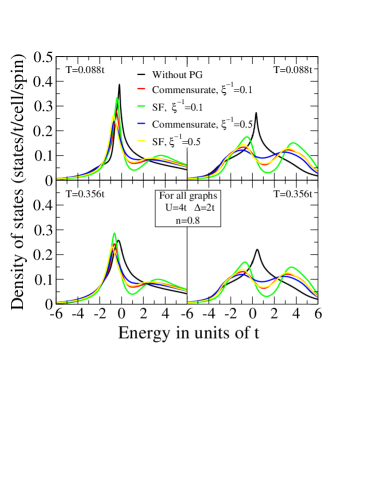
Figure 1: Comparison of DOSs obtained from DMFT(NRG)+$\Sigma_{\bf k}$ calculations for different combinatorical factors (SF — spin–fermion model, commensurate), inverse correlation lengths ($\xi^{-1}$) in units of the lattice constant, temperatures ($T$) and pseudogap potential $\Delta=2t$. Left column corresponds to $t^{\prime}/t=-0.4$, right column to $t^{\prime}=0$. In all graphs the Coulomb interaction is $U=4t$ and $n=0.8$. The Fermi level corresponds to zero.

Let us start the discussion of results obtained within our generalized DMFT+$\Sigma_{\bf k}$ approach with the densities of states (DOSs) for the case of small (relative to bandwidth) Coulomb interaction $U=4t$ with and without pseudogap fluctuations. As already discussed in the Introduction, the characteristic feature of the strongly correlated metallic state is the coexistence of lower and upper Hubbard bands split by the value of $U$ with a quasiparticle peak at the Fermi level. Since at half–filling the bare DOS of the square lattice has a Van–Hove singularity at the Fermi level ($t^{\prime}=0$) or close to it (in case of $t^{\prime}/t=-0.4$) one cannot treat a peak on the Fermi level simply as a quasiparticle peak. In fact, there are two contributions to this peak from (i) the quasiparticle peak appearing in strongly correlated metals due to many-body effects and (ii) the smoothed Van–Hove singularity from the bare DOS. In Fig. 1 we show the corresponding DMFT(NRG) DOSs without pseudogap fluctuations as black lines for $n=0.8$ for both bare dispersions $t^{\prime}/t=-0.4$ (left panels) and for $t^{\prime}=0$ (right panels) for two different temperatures $T=0.356t$ (middle panels) and $T=0.088t$ (upper and lower panels). The remaining curves in Fig. 1 represent results for the DOSs with non-local fluctuations switched on. For all sets of parameters one can see that the introduction of non-local fluctuations into the calculation leads to the formation of pseudogap within the quasiparticle peak.

For $n=0.8$ (Fig. 1) the picture of DOS is slightly asymmetric. The width of the pseudogap (the distance between peaks closest to Fermi level) appears to be of the order of $\sim 2\Delta$. We have checked that decreasing the value of $\Delta$ from $2t$ to $t$ leads to a pseugogap that is correspondingly twice smaller and in addition more shallow. When one uses the combinatorial factors corresponding to the spin–fermion model (Eq.(12)), the pseudogap becomes more pronounced than in the case of commensurate charge fluctuations (combinatorial factors of Eq. (11)). The influence of the correlation length $\xi$ is also as expected. Changing $\xi^{-1}$ from $\xi^{-1}=0.1$ to $\xi^{-1}=0.5$, i.e. decreasing the range of the non-local fluctuations, slightly washes out the pseudogap. Also, increasing the temperature from $T=0.088t$ to $T=0.356t$ leads to a general broadening of the structures in the DOSs. Noteworthy is the fact that for $t^{\prime}/t=-0.4$ and $\xi^{-1}=0.5$ the pseudogap has almost disappeared for the temperatures studied here. Also very remarkable point is the similarity of the results obtained with the generalized DMFT+$\Sigma_{\bf k}$ approach with $U=4t$ (smaller than the bandwidth $W$) to those obtained earlier without Hubbard–like Coulomb interactions Sch ; KS .

Let us now consider the case of a doped Mott insulator. The model parameters are again taken as $t^{\prime}/t=-0.4$ with filling factor of $n=0.8$, but the Coulomb interaction strength is set to $U=40t$. Characteristic features of the DOS for such a strongly correlated metal are a strong separation of lower and upper Hubbard bands and a Fermi level crossing by the lower Hubbard band (for non–half–filled case). Without non-local fluctuations the quasi–particle peak is again formed at the Fermi level, but now the upper Hubbard band is far to the right and does not touch the quasiparticle peak (as it was for the case of small Coulomb interactions).

Pseudogap appears close to the middle of quasiparticle peak. In addition we observe that the lower Hubbard band is slightly broadened by fluctuation effects. Qualitative behaviour of the pseudogap anomalies is similar to those described above for the case of $U=4t$, e.g. a decrease of $\xi$ makes the pseudogap less pronounced, while reducing $\Delta$ from $\Delta=2t$ to $\Delta=t$ narrows of the pseudogap and also makes it more shallow. Note that for the doped Mott–insulator the pseudogap is remarkably more pronounced for the SDW–like fluctuations than for CDW–like fluctuations.

There are, however, quite clear differences to the case of $U=4t$. For example, the width of the pseudogap appears to be much smaller than $2\Delta$, which we attribute to the fact that the quasiparticle peak itself is actually rather narrow in the case of doped Mott insulator.

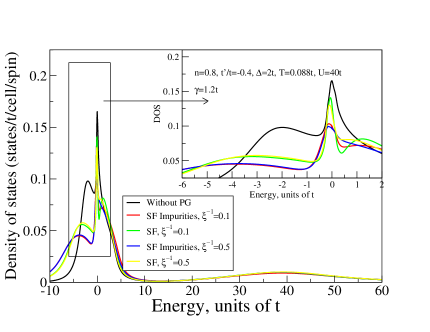
Figure 3: Comparison of DOSs obtained from DMFT(NRG)+$\Sigma_{\bf k}$ calculations for $t^{\prime}/t=-0.4$, $T=0.088t$, $U=40t$, $n=0.8$ and for impurity scattering rate $\gamma=1.2t$.

Random impurity scattering, in general case leads to the filling of the pseudogap with the growth of impurity scattering rate both for correlated metal and doped Mott insulator. As a typical example, in Fig. 3 we show results of our calculations for the case of doped Mott insulator. These were obtained via non self–consistent procedure (using (16), (17), as full self–consistent procedure leads only to rather insignificant quantitative changes.

IV.3 Generalized DMFT+$\Sigma_{\bf k}$ approach: spectral functions $A(\omega,{\bf k})$

In the previous subsection we discussed the densities of states obtained self–consistently by the DMFT+$\Sigma_{\bf k}$ approach. Once we get a self–consistent solution of the DMFT+$\Sigma_{\bf k}$ equations with non-local fluctuations we can, of course, also compute the spectral functions $A(\omega,{\bf k})$

$$A(\omega,{\bf k})=-\frac{1}{\pi}{\rm Im}\frac{1}{\omega+\mu-\varepsilon({\bf k})-\Sigma(\omega)-\Sigma_{\bf k}(\omega)},$$ (19)

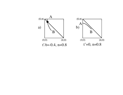
Figure 4: 1/8-th of the bare Fermi surfaces for the different occupancies $n$ and combinations ($t,t^{\prime}$) used for the calculation of spectral functions $A({\bf k},\omega)$. The diagonal line corresponds to the antiferromagnetic Brillouin zone boundary at half–filling for a square lattice with nearest-neighbours hopping only. The full circle marks the so-called “hot–spot”.

where self–energy $\Sigma(\omega)$ and chemical potential $\mu$ are calculated self–consistently as described in Sec. II. To plot $A(\omega,{\bf k})$ we choose ${\bf k}$–points along the “bare” Fermi surfaces for different types of lattice spectra and fillings. In Fig. 4 one can see corresponding shapes of these “bare” Fermi surfaces (presented are only 1/8-th parts of the Fermi surfaces within the first quadrant of the Brillouin zone).

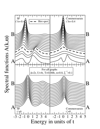
Figure 5: Spectral functions $A({\bf k},\omega)$ obtained from the DMFT(NRG)+$\Sigma_{\bf k}$ calculations along the directions shown in Fig. 4. Model parameters were chosen as $U=4t$, $n=0.8$, $\Delta=2t$, $\xi^{-1}=0.1$ and temperature $T=0.088t$. The “hot–spot” k-point is marked as fat dashed line. The Fermi level corresponds to zero.

In the following we concentrate mainly on the case $U=4t$ and filling $n=0.8$ (Fermi surface of Fig. 4(a)). The corresponding spectral functions $A(\omega,{\bf k})$ are depicted in Fig. 5. When $t^{\prime}/t=-0.4$ (upper row), the spectral function close to the Brillouin zone diagonal (point B) has the typical Fermi–liquid behaviour, consisting of a rather sharp peak close to the Fermi level. In the case of SDW–like fluctuations this peak is shifted down in energy by about $-0.5t$ (left upper corner). In the vicinity of the “hot–spot” the shape of $A(\omega,{\bf k})$ is completely modified. Now $A(\omega,{\bf k})$ becomes double–peaked and non–Fermi–liquid–like. Directly at the “hot–spot”, $A(\omega,{\bf k})$ for SDW–like fluctuations has two equally intensive peaks situated symmetrically around the Fermi level and split from each other by $\sim 1.5\Delta$ Refs. Sch ; KS . For commensurate CDW–like fluctuations the spectral function in the “hot–spot” region has one broad peak centered at the Fermi level with width $\sim\Delta$. Such a merging of the two peaks at the “hot–spot” for commensurate fluctuations was previously observed in Ref. KS . However close to point A this type of fluctuations also produces a double–peak structure in the spectral function.

In the lower panel of Fig. 5 we show spectral functions hole doping ($n=0.8$) and the case of $t^{\prime}=0$ (Fermi surface from Fig. 4(b)). Since the Fermi surface now is everywhere close to the antiferromagnetic zone boundary, the pseudogap anomalies are rather strong and almost non–dispersive along the Fermi surface.

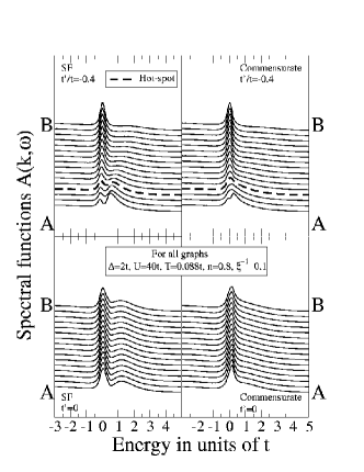
Figure 6: Spectral functions $A({\bf k},\omega)$ obtained from the DMFT(NRG)+$\Sigma_{\bf k}$ calculations for $U=40t$, other parameters as in Fig. 5.

For the case of a doped Mott insulator ($U=40t$, $n=0.8$), the spectral functions obtained by the DMFT+$\Sigma_{\bf k}$ approach are presented in Fig. 6. Qualitatively, the shapes of these spectral functions are similar to those shown on Fig. 5. As was pointed out above, the strong Coulomb correlations lead to a narrowing of the quasiparticle peak and a corresponding decrease of the pseudogap width. One should also note that in contrast to $U=4t$ the spectral functions are now less intensive, because part of the spectral weight is transferred to the upper Hubbard band.

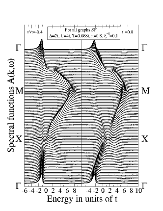
Figure 7: Spectral functions $A({\bf k},\omega)$ obtained from the DMFT(NRG)+$\Sigma_{\bf k}$ calculations along high-symmetry directions of first Brilloin zone $\Gamma(0,0)\!-\!\rm{X}(\pi,0)\!-\!\rm{M}(\pi,\pi)\!-\!\Gamma(0,0)$, SF combinatorics (left row) and commensurate combinatorics (right column). Other parameters are $U=4t$, $n=0.8$, $\Delta=2t$, $\xi^{-1}=0.1$ and temperature $T=0.088t$. The Fermi level corresponds to zero.

Using another quite common choice of ${\bf k}$–points we can compute $A(\omega,{\bf k})$ along high–symmetry directions in the first Brillouin zone: $\Gamma(0,0)\!-\!\rm{X}(\pi,0)\!-\!\rm{M}(\pi,\pi)\!-\!\Gamma(0,0)$. The spectral functions for these ${\bf k}$–points are shown in Fig.  7 for the case of SDW–like fluctuations and $U=4t$. For all sets of parameters one can see a characteristic double – peak pseudogap structure close to the $X$ point. In the middle of $M\!-\!\Gamma$ direction (so called “nodal” point) one can see the reminiscence of AFM gap which has its biggest value here in case of perfect antiferromagnetic ordering. Also in the nodal point “kink”-like behavior is observed caused by interactions between correlated electrons with pseudo-gap fluctuations. A change of the filling leads mainly to a rigid shift of spectral functions with respect to the Fermi level. For the case of $U=40t$ spectral densities demonstrate rather similar behavior cm05 .

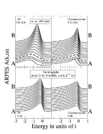
Figure 8: ARPES spectra obtained from the DMFT(NRG)+$\Sigma_{\bf k}$ calculations for $U=4t$ and $n=0.8$ along the lines in the first BZ as depicted by Fig. 4, all other parameters as in Fig. 5.

With the spectral functions we are now in a position to calculate angle resolved photoemission spectra (ARPES), which is the most direct experimental way to observe pseudogap in real compounds. For that purpose, we only need to multiply our results for the spectral functions with the Fermi function at appropriate temperature. Typical example of the resulting DMFT+$\Sigma_{\bf k}$ ARPES spectra are presented in Fig. 8. One should note that for $t^{\prime}/t=-0.4$ (upper panel of Fig. 8) as ${\bf k}$ goes from point “A” to point “B” the peak situated slightly below the Fermi level changes its position and moves down in energy. Simultaneously it becomes more broad and less intensive. The dotted line guides the motion of the peak maximum. Such behaviour of the peak in the ARPES is rather reminiscent of those observed experimentally in underdoped cuprates MS ; Sch ; Kam .

IV.4 “Destruction” of the Fermi surface

Within the standard DMFT approach Fermi surface is not renormalized by interactions and just coincides with that of the “bare” quasiparticles vollha93 . However, in the case of nontrivial momentum dependence of electron self – energy, important renormalization of the Fermi surface appears due to pseudogap formation Sch . There are a number of ways to define Fermi surface in strongly correlated system with pseudogap fluctuations. In the following we are using intensity plots (within the Brillouin zone) of the spectral density (19) taken at $\omega=0$. These are readily measured by ARPES and appropriate peak positions define the Fermi surface in the usual Fermi liquid case.

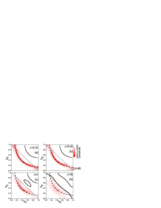
Figure 9: Fermi surfaces obtained from the DMFT(NRG)+$\Sigma_{\bf k}$ calculations for $U=4t$ and $n=0.8$. Shown are intensity plots of spectral density (19) for $\omega=0$ and $\xi=10a$. (a) – $\Delta=0.2t$; (b) – $\Delta=0.4t$; (c) – $\Delta=t$; (d) – $\Delta=2t$. Dashed line denotes “bare” Fermi surface. Black lines show the solution of Eq. (20).

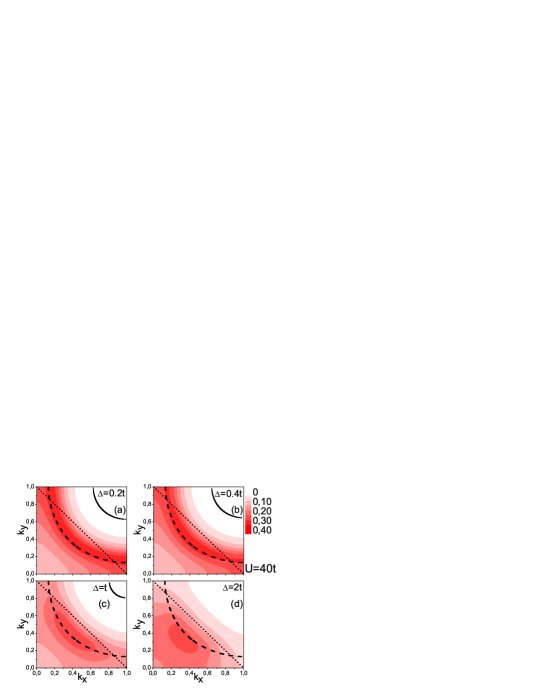
Figure 10: “Destruction”of the Fermi surface obtained from the DMFT(NRG)+$\Sigma_{\bf k}$ calculations for $U=40t$ and $n=0.8$. Other parameters and notations are the same as in Fig. 9.

Our results KNS are shown in Fig. 9 for the case of correlated metal with $U=4t$ and in Fig. 10 for the doped Mott insulator ($U=40t$) (in both cases we assume spin – fermion combinatorics). The qualitative behavior observed in Fig. 9 clearly demonstrates the “destruction” of the well defined Fermi surface in the strongly correlated metal with the growth of the pseudogap amplitude $\Delta$. Quite similar behavior was first observed in pioneering paper by Norman et al.Norm and in numerous later ARPES experiments. It is seen, that “destruction” of the Fermi surface starts in the vicinity of “hot spots” for small values of $\Delta$, but almost immediately it disappears in the whole antinodal region of the Brillouin zone, while only “Fermi arcs” remain in the nodal region very close to the “bare” Fermi surface. These results give a natural explanation of the observed behavior and also of the fact that the existence of “hot spots” regions was observed only in some rare cases Arm .

For the case of doped Mott insulator shown in Fig. 10 we see that the Fermi surface is rather poorly defined for all values of $\Delta$, as the spectral density profiles are much more “blurred” than in the case of smaller values of $U$, reflecting important role of correlations.

It is interesting to note that from Figs. 9, 10 it is clearly seen that rather natural definition of the Fermi surface as defined by the solution of the equation

$$\omega-\varepsilon({\bf k})+\mu-Re\Sigma(\omega)-Re\Sigma_{\bf k}(\omega)=0$$ (20)

for $\omega=0$, used e.g. in Ref.Sch is inadequate for strongly correlated systems with finite $U$ and nonlocal interactions (pseudogap fluctuations).

V Conclusion

To summarize, we propose a generalized DMFT+$\Sigma_{\bf k}$ approach, which is meant to take into account the important effects due to non–local correlations in a systematic, but to some extent phenomenological fashion. The main idea of this extension is to stay within a usual effective Anderson impurity analogy, and introduce length scale dependence due to non-local correlation via the effective medium (“bath”) appearing in the standard DMFT. This becomes possible by incorporating scattering processes of fermions in the “bath” from non–local collective SDW–like antiferromagnetic spin (or CDW–like charge) fluctuations. Such a generalization of the DMFT allows one to overcome the well–known shortcoming of ${\bf k}$–independence of self–energy of the standard DMFT. It in turn opens the possibility to access the physics of low–dimensional strongly correlated systems, where different types of spatial fluctuations (e.g. of some order parameter), become important. However, we must stress that our procedure in no way introduces any kind of systematic $1/d$–expansion, being only a qualitative method to include length scale into DMFT.

In our present study we addressed the problem of pseudogap formation in the strongly correlated metallic state. We showed evidence that the pseudogap appears at the Fermi level within the quasiparticle peak, introducing a new small energy scale of the order of $\Delta$ in the DOSs and spectral functions $A(\omega,{\bf k})$ and significant renormalization of the Fermi surface.

Let us stress, that our generalization of DMFT leads to non–trivial and in our opinion physically sensible ${\bf k}$–dependence of spectral functions. Similar results were obtained in recent years using the cluster mean-field theories TMrmp . The major advantage of our approach over these theories is, that we stay in an effective single-impurity picture. This means that our approach is computationally much less expensive and therefore also easily generalizable for the account of additional interactions .

VI Acknowledgements

We are grateful to Th. Pruschke for providing us with his NRG code and helpful discussions. This work was supported in part by RFBR grants 05-02-16301, 05-02-17244, and programs of the Presidium of the Russian Academy of Sciences (RAS) “Quantum macrophysics” and of the Division of Physical Sciences of the RAS “Strongly correlated electrons in semiconductors, metals, superconductors and magnetic materials”. I.N. acknowledges support from the Dynasty Foundation and International Centre for Fundamental Physics in Moscow program for young scientists 2005 and Russian Science Support Foundation program for young PhD of the Russian Academy of Sciences 2005.

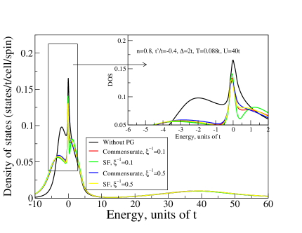
Figure 2: Comparison of DOSs obtained from DMFT(NRG)+$\Sigma_{\bf k}$ calculations for $t^{\prime}/t=-0.4$, $T=0.088t$, $U=40t$ and filling $n=0.8$.

References

- (1) T. Timusk, B. Statt, Rep. Progr. Phys, 62, 61 (1999).
- (2) M. V. Sadovskii, Usp. Fiz. Nauk 171, 539 (2001) [Physics – Uspekhi 44, 515 (2001)].
- (3) D. Pines, ArXiv: cond-mat/0404151.
- (4) J. Schmalian, D. Pines, B.Stojkovic, Phys. Rev. B 60, 667 (1999).
- (5) E. Z. Kuchinskii, M. V. Sadovskii, Zh. Eksp. Teor. Fiz. 115, 1765 (1999) [(JETP 88, 347 (1999)].
- (6) W. Metzner and D. Vollhardt, Phys. Rev. Lett. 62, 324 (1989).
- (7) D. Vollhardt, in Correlated Electron Systems, edited by V. J. Emery, World Scientific, Singapore, 1993, p. 57.
- (8) Th. Pruschke, M. Jarrell, and J. K. Freericks, Adv. in Phys. 44, 187 (1995).
- (9) A. Georges, G. Kotliar, W. Krauth, and M. J. Rozenberg, Rev. Mod. Phys. 68, 13 (1996).
- (10) G. Kotliar and D. Vollhardt, Physics Today 57, No. 3 (March), 53 (2004).
- (11) M.V. Sadovskii, I.A. Nekrasov, E.Z. Kuchinskii, Th. Prushke, V.I. Anisimov. Phys. Rev. B 72, 155105 (2005)
- (12) M. V. Sadovskii, Zh. Eksp. Teor. Fiz. 77, 2070(1979) [Sov.Phys.–JETP 50, 989 (1979)].
- (13) Y. M. Vilk, A.-M. S. Tremblay, J. Phys. I France 7, 1309 (1997).
- (14) N.A.Kuleeva, E.Z.Kuchinskii, M.V.Sadovskii, Zh. Eksp. Teor. Fiz. 126, 1446 (2004) [JETP 99, 1264 (2004)]
- (15) J. E. Hirsch and R. M. Fye, Phys. Rev. Lett. 56, 2521 (1986); M. Jarrell, Phys. Rev. Lett. 69, 168 (1992); M. Rozenberg, X. Y. Zhang, and G. Kotliar, Phys. Rev. Lett. 69, 1236 (1992); A. Georges and W. Krauth, Phys. Rev. Lett. 69, 1240 (1992); M. Jarrell in Numerical Methods for lattice Quantum Many-Body Problems, edited by D. Scalapino, Addison Wesley, 1997. For review of QMC for DMFT see Ref.Held01 .
- (16) K. Held, I.A. Nekrasov, N. Blümer, V.I. Anisimov, and D. Vollhardt, Int. J. Mod. Phys. B 15, 2611 (2001); K. Held, I.A. Nekrasov, G. Keller, V. Eyert, N. Blümer, A.K. McMahan, R.T. Scalettar, T. Pruschke, V.I. Anisimov, and D. Vollhardt, cond-mat/0112079 (Published in Quantum Simulations of Complex Many-Body Systems: From Theory to Algorithms, eds. J. Grotendorst, D. Marks, and A. Muramatsu, NIC Series Volume 10 (NIC Directors, Forschunszentrum Jülich, 2002) p. 175-209.
- (17) K.G. Wilson, Rev. Mod. Phys. 47, 773 (1975); H.R. Krishna-murthy, J.W. Wilkins, and K.G. Wilson, Phys. Rev. B 21, 1003 (1980); ibid. 21, 1044 (1980); for a comprehensive introduction to the NRG see e.g. A.C. Hewson, The Kondo Problem to Heavy Fermions (Cambridge University Press, 1993).
- (18) R. Bulla, A.C. Hewson and Th. Pruschke, J. Phys. – Condens. Matter 10, 8365(1998); R. Bulla, Phys. Rev. Lett. 83, 136 (1999).
- (19) A. Kaminski, H. M. Fretwell, M. R. Norman, M. Randeria, S. Rosenkranz, U. Chatterjee, J. C. Campuzano, J. Mesot, T. Sato, T. Takahashi, T. Terashima, M. Takano, K. Kadowaki, Z. Z. Li, H. Raffy, Phys. Rev. B 71, 014517 (2005).
- (20) E.Z.Kuchinskii, I.A.Nekrasov, M.V.Sadovskii. JETP Lett. 82, 198 (2005)
- (21) M.R. Norman, M. Randeria, J.C. Campuzano, T.Yokoya, T. Takeuchi, T. Takahashi, T. Mochiku, K. Kadowaki, P. Guptasarma, D.G. Hinks, Nature 382, 51 (1996)
- (22) N.P. Armitage, D.H. Lu, C. Kim, A. Damascelli, K.M. Shen, F. Ronning, D.L. Feng, P. Bogdanov, Z.-X. Shen. Phys. Rev. Lett. 87, 147003 (2001)
- (23) Th. Maier, M. Jarrell, Th. Pruschke and M. Hettler, Rev. Mod. Phys. (in print), ArXiv: cond-mat/0404055.