Quantum chaos in nanoelectromechanical systems

Abstract

We present a theoretical study of the electron-phonon coupling in suspended nanoelectromechanical systems (NEMS) and investigate the resulting quantum chaotic behavior. The phonons are associated with the vibrational modes of a suspended rectangular dielectric plate, with free or clamped boundary conditions, whereas the electrons are confined to a large quantum dot (QD) on the plate’s surface. The deformation potential and piezoelectric interactions are considered. By performing standard energy-level statistics we demonstrate that the spectral fluctuations exhibit the same distributions as those of the Gaussian Orthogonal Ensemble (GOE) or the Gaussian Unitary Ensemble (GUE), therefore evidencing the emergence of quantum chaos. That is verified for a large range of material and geometry parameters. In particular, the GUE statistics occurs only in the case of a circular QD. It represents an anomalous phenomenon, previously reported for just a small number of systems, since the problem is time-reversal invariant. The obtained results are explained through a detailed analysis of the Hamiltonian matrix structure.

I Introduction

The possibility of engineering devices at the nano and micro scales has created the conditions for testing fundamental aspects of quantum theory Brandes , otherwise difficult to probe in natural atomic size systems. In particular, quantum dots (QD) have largely been considered as a physical realization of quantum billiards Berggren ; Bruus ; Beenakker and mesoscopic structures have played an important role in the experimental study of quantum chaos Stockmann , mainly through the investigation of the transport properties of quantum dot Marcus and quantum well Fromhold structures in the presence of magnetic field. However, some extraneous effects can prevent the full observation of the quantum chaotic behavior. For instance, impurities and soft confining potentials may mask the chaotic dynamics predicted for some semiconductor quantum billiards (e.g., the stadium)Berggren and the incoherent influence of the bulk on the electronic dynamics hinders the observation of the so called eigenstate scars Heller in quantum corrals Crommie . Furthermore, Random Matrix Theory (RMT) predictions for the Coulomb blockade peaks in quantum dots may fail as a result of the coupling with the environment Madger .

Alternatively, suspended nanostructures are ideal candidates for implementing and investigating coherent phenomena in semiconductor devices, because, at low temperatures, they provide excellent isolation for the quantum system from the bulk of the sample nano ; Blencowe . The nanoelectromechanical systems (NEMS), in particular, are specially suited to study the effects of a phonon bath on the electronic states, possibly leading to a chaotic behavior. Such point is of practical relevance since it bears the question of the stability of quantum devices Chuang ; Cleland , whose actual implementation could be prevented by the emergence of chaos Georgeot .

In a recent paper rego , we have shown that in fact suspended nanostructures can display quantum chaotic behavior. In this article we extend such studies and perform a detailed analysis of the coupling between the phonons of a suspended nanoscopic dielectric plate and the electrons of a two-dimensional electron gas (2DEG). The phonons are associated with the vibrational modes of a suspended rectangular plate (i.e., the phonon cavity) and the 2DEG (in the free electron approximation) is confined to a large quantum dot (billiard) built on the plate’s surface.

Two different scenarios are considered for the shape of the quantum dot: circular and rectangular geometries (Fig. 1), which yield distinct chaotic features. As for the coupling mechanisms, we take into account the deformation and piezoelectric potentials. By performing energy-level statistics we show that, for sufficiently strong electron-phonon coupling, such electromechanical nanostructures can exhibit quantum chaos for a large range of material and geometry parameters. The resulting spectral correlation functions, which depend on the geometry and location of the center of the QD on the surface of the plate as well as on the plate’s boundary conditions (free or clamped), are those expected from the Gaussian Orthogonal Ensemble (GOE) or Gaussian Unitary Ensemble (GUE) of the Random Matrix Theory (RMT) Mehta . We present a detailed explanation for the occurrence of such different statistics distributions. Noteworthy are the results for the circular QD, since in this case the GUE statistics can be obtained in spite of the fact that the system is time-reversal invariant. By investigating the influence of material and geometrical parameters on the unfolding of chaos, we indicate the conditions for its experimental observation.

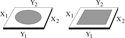
Figure 1: Schematics of the suspended nanoelectromechanical structures depicting the cases of a circular and a rectangular quantum dot on the surface of a suspended dielectric plate.

II The system Hamiltonian

The full Hamiltonian of the problem is composed of three parts: the phonons, the electrons and the electron-phonon interactions, which are formulated in the sequence.

II.1 Phonons

At temperatures below 1 Kelvin the acoustic phonon mean free path in SiN (silicon nitride), for instance, can be as large as 10 $\mu$m phonongas . This implies that a plane wave acoustic phonon propagating through a suspended mesoscopic system whose dimensions are much smaller than this mean free path hits the boundaries many times during its expected lifetime, giving rise to standing waves. Thus, the phonons in such systems can be described in terms of the plate’s normal modes of deflection, instead of the plane wave phonon description that is more appropriate for bulk systems. Therefore, in the following we associate the phonons with the vibrational modes of the suspended mesoscopic system. In addition, at low temperatures the semiconductor can be treated as a continuum elastic material due to the large wavelength of the phonons.

To obtain the long wavelength vibrational modes of the plate we use the Classical Plate Theory (CPT) approximation Graff . The CTP describes adequately the vibrations of a plate whose thickness is much smaller than its lateral dimensions, which is the characteristic of our NEMS. The deflections of a plate lying in the $(x,y)$ plane are thus described by a vector field $\left[U({\bf r})\,\hat{\imath}+V({\bf r})\,\hat{\jmath}+W({\bf r})\,\hat{k}\right]\exp(-i\omega t)$ of components

$$U(x,y,z)=-z\frac{\partial W}{\partial x},\ \ V(x,y,z)=-z\frac{\partial W}{\partial y}\ ,$$ (1)

$$W(x,y)=\sum_{m,n}A_{mn}X_{m}(x)Y_{n}(y).$$ (2)

In Eq. (2), $W(x,y)$ is written in terms of the one-dimensional transverse modes $X_{m}$ and $Y_{n}$, which are the solutions of the Bernoulli-Euler equation Graff ; Leissa under the appropriate boundary conditions. Considering that each of the four sides of the plate can be either clamped (C) or free (F) (corresponding to the Dirichlet or Neumann boundary conditions, respectively), we have

$$X_{m}(x) = \sin[k_{m}x]\pm\sinh[k_{m}x]$$ (3)

$$+\zeta\left\{\cos[k_{m}x]\pm\cosh[k_{m}x]\right\}\ ,$$

where

$$\zeta=\frac{\cos[k_{m}L_{x}]-\cosh[k_{m}L_{x}]}{\sin[k_{m}L_{x}]+\sinh[k_{m}L_{x}]}.$$ (4)

Likewise for $Y_{n}(y)$. The signs in Eq. (3) are positive (negative) for the FF (CC and CF) boundary conditions orthonormal . The $k_{m}$’s are solutions of $\cos[kL_{x}]\cosh[kL_{x}]=1$.

Under given boundary conditions, the Rayleigh-Ritz method is used to obtain the coefficients $A_{mn}^{\alpha}$ of Eq. (2) and the eigenfrequencies $\omega_{\alpha}$ corresponding to the eigenmode ${\bf u}_{\alpha}({\bf r})$ of the plate. It is done by imposing $\partial\mathcal{U}/\partial A_{mn}=0$ to the energy functional ${\cal{U}}=\int dxdy\,[{\cal{K}}(x,y)-{\cal{V}}(x,y)]$ Leissa , where the kinetic and strain energies are written as

$${\cal{K}}(x,y) = \rho_{{}_{2D}}\frac{\omega^{2}}{2}W^{2}(x,y),$$ (5)

$${\cal{V}}(x,y) = \frac{D}{2}\left(\frac{\partial^{2}W}{\partial x^{2}}+\frac{\partial^{2}W}{\partial y^{2}}\right)-(1-\nu)D$$ (6)

$$\times\left(\frac{\partial^{2}W}{\partial x^{2}}\frac{\partial^{2}W}{\partial y^{2}}-\left(\frac{\partial^{2}W}{\partial x\partial y}\right)^{2}\right).$$

Here $\rho_{{}_{2D}}$ denotes the two-dimensional density, $\nu$ is the Poisson constant and $D$ is the rigidity constant.

In the CPT approximation, the most important motion is that in the $z$ direction, given by $W(x,y)$, whereas the displacements along the $x$ and $y$ directions are described approximately by the first term of an orthogonal basis expansion. Therefore, an arbitrary transverse motion can be expanded in the basis of the orthonormal vibrational modes $W_{\alpha}(x,y)$, for which

$$\langle W_{\alpha}(x,y)|W_{\beta}(x,y)\rangle=\delta_{\alpha\beta},$$

$$\sum_{\alpha}W_{\alpha}(x,y)W_{\alpha}(x^{\prime},y^{\prime})=\delta(x-x^{\prime})\delta(y-y^{\prime}).$$ (7)

The $U_{\alpha}$ and $V_{\alpha}$ components are only approximately orthonormal. As an illustration, we show in Fig. 2 the vector field components $(U_{\alpha},V_{\alpha},W_{\alpha})$ of the SA2 eigenmode (i.e., the second symmetric/antisymmetric eigenmode) for the {FFFF} boundary conditions. Hereafter, we refer to the set of boundary conditions of the plate, either C or F, as {$X_{1}X_{2}Y_{1}Y_{2}$}, in accordance to Fig. 1.

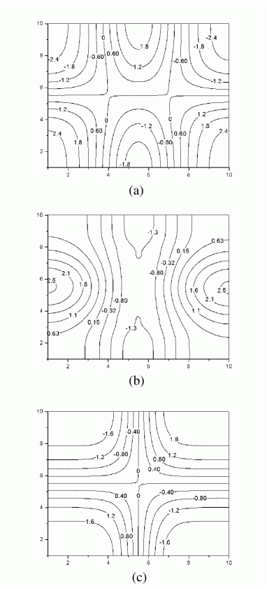
Figure 2: Contour plots for the cavity deflection mode SA2 (the second symmetric/antisymmetric eigenmode) for the {FFFF} boundary conditions, calculated at the surface of the plate: (a) $W(x,y)$, (b) $U(x,y)$, and (c) $V(x,y)$. The amplitudes and lateral dimensions are given in arbitrary units.

An arbitrary vibration field of the cavity is written in terms of its deflection modes $\alpha$ as

$${\bf u}({\bf r},t) = \sum_{\alpha}\left[Q_{\alpha}(t)+Q^{*}_{\alpha}(t)\right]$$ (8)

$$\times\left[U_{\alpha}({\bf r})\,\hat{\imath}+V_{\alpha}({\bf r})\,\hat{\jmath}+W_{\alpha}({\bf r})\,\hat{k}\right],$$

together with the normal coordinates $Q_{\alpha}(t)=Q_{\alpha}\exp[-i\omega_{\alpha}t]$. In writing Eq. (8), we have taken into account that the modes $\alpha$ are real.

To provide the same level of description for the elastic and electronic degrees of freedom of the electromechanical nanostructure, we perform the canonical quantization of the vibration field given by Eq. (8). As a result, we associate the classical field ${\bf u}({\bf r},t)$ with the quantum operator $\hat{{\bf u}}({\bf r},t)$, which must satisfy the equal-time commutation relation $[{\bf\hat{u}}_{j}({\bf r},t),{\bf\hat{\pi}}_{j}({\bf r^{\prime}},t)]=i\hbar\delta({\bf r-r^{\prime}})$, with the conjugate momentum operator ${\bf\hat{\pi}}({\bf r},t)=m\partial_{t}{\bf\hat{u}}$. Particularly, for the $\hat{k}$ component of the field we have

$$[W(x,y),\pi_{z}(x,y)]=i\hbar\delta(x-x)\delta(y-y).$$ (9)

But if we write ($\mathcal{X}_{\alpha}(t)\equiv\left[\hat{Q}_{\alpha}(t)+\hat{Q}_{\alpha}^{\dagger}\right]$)

$$W(x,y,t) = \sum_{\alpha}\mathcal{X}_{\alpha}(t)W_{\alpha},$$

$$\pi_{z}(x,y,t) = \rho V\sum_{\alpha}(-i\omega_{\alpha})\mathcal{X}_{\alpha}(t)W_{\alpha}=\sum_{\alpha}\mathcal{P}_{\alpha}(t)W_{\alpha},$$

the commutation relation (9) yields

$$[W(x,y),\pi_{z}(x,y)]=\sum_{\alpha,\beta}[\mathcal{X}_{\alpha},\mathcal{P}_{\beta}]W_{\alpha}W_{\beta}.$$ (11)

Then, by requiring that $[\mathcal{X}_{\alpha},\mathcal{P}_{\beta}]=i\hbar\delta_{\alpha,\beta}$ one can use Eq. (7) to show that Eq. (9) is satisfied. Thus, $\mathcal{X}_{\alpha}$ and $\mathcal{P}_{\alpha}$ are canonically conjugated operators, satisfying $[\mathcal{X}_{\alpha},\mathcal{X}_{\beta}]=[\mathcal{P}_{\alpha},\mathcal{P}_{\beta}]=0$ as well.

The normal coordinates are now the quantum mechanical operators $\hat{Q}_{\alpha}(t)$ and $\hat{Q}_{\alpha}^{\dagger}(t)$, which are used to define the dimensionless number operators

$$a^{\dagger}_{\alpha}=\sqrt{\frac{2V\rho\omega_{\alpha}}{\hbar}}\hat{Q}^{\dagger}_{\alpha},\qquad a_{\alpha}=\sqrt{\frac{2V\rho\omega_{\alpha}}{\hbar}}\hat{Q}_{\alpha}.$$ (12)

From the previous commutation relations it can be shown that $[a_{\alpha}(t),a_{\beta}^{\dagger}(t)]=\delta_{\alpha,\beta}$ and $[a_{\alpha},a_{\alpha^{\prime}}]=[a^{\dagger}_{\alpha},a^{\dagger}_{\alpha^{\prime}}]=0$. Therefore, $a^{\dagger}_{\alpha}$ and $a_{\alpha}$ are the creation and annihilation operators of the phonon deflection modes $\alpha$ and the vibration field operator ${\bf\hat{u}}({\bf r},t)$ is

$$\hat{{\bf u}}=\sum_{\alpha}\frac{[a_{\alpha}(t)+a^{\dagger}_{\alpha}(t)]}{\sqrt{2\ V\rho\ \omega_{\alpha}/\hbar}}\left[U_{\alpha}({\bf r})\,\hat{\imath}+V_{\alpha}({\bf r})\,\hat{\jmath}+W_{\alpha}({\bf r})\,\hat{k}\right].$$ (13)

II.2 Electrons

We consider the free electron approximation and assume the electrons to be completely confined to a narrow quantum dot, forming a quasi-2DEG of thickness $d$. The normalized electronic eigenstates are written as $\phi_{\kappa,\gamma}({\bf r})=\varphi_{\kappa}(x,y)\sqrt{2/d}\sin[\gamma\pi z/d]$. Due to the quasi-2D assumption, the electrons always occupy the lowest state in the $z$ direction, so in our calculations we set the quantum number $\gamma=1$.

For the rectangular QD of sides $L_{x}$ and $L_{y}$, we have

$$\varphi_{\kappa}(x,y)=\frac{2}{\sqrt{L_{x}L_{y}}}\sin[\frac{p\pi x}{L_{x}}]\sin[\frac{q\pi y}{L_{y}}],$$ (14)

with $\kappa\equiv(p,q)$ and $p,q$ assuming positive integer values. The corresponding eigenenergies are

$$E_{\kappa,\gamma=1}=\frac{\pi^{2}\hbar^{2}}{2m_{e}}\left(\frac{p^{2}}{L_{x}^{2}}+\frac{q^{2}}{L_{y}^{2}}+\frac{1}{d^{2}}\right),$$ (15)

where $m_{e}$ is the effective electron mass in the QD.

For the circular QD of radius $R$, we have

$$\varphi_{\kappa}(r,\theta)=\frac{{\mbox{J}}_{|l|}\left(\alpha_{l\nu}\frac{r}{R}\right)\exp[i\,l\,\theta]}{\sqrt{\pi}R|J_{|l|+1}(\alpha_{l\nu})|},$$ (16)

with $\kappa\equiv(l,\nu)$, $l=0,\pm 1,\pm 2,\ldots$ and $\alpha_{l\nu}$ the $\nu$-th root of the Bessel function of order $|l|$. Here, the eigenenergies are

$$E_{\kappa,\gamma=1}=\frac{\hbar^{2}}{2m_{e}}\left(\frac{\alpha_{l\nu}^{2}}{R^{2}}+\frac{\pi^{2}}{d^{2}}\right).$$ (17)

II.3 Electron-phonon interactions

The electrons interact with the lattice vibrations through different mechanisms, depending on the characteristics of the solid and the temperature. In addition, from the theoretical point of view there can be several approaches to describe the coupling between electrons and phonons. Next we formulate the electron-phonon interaction terms that are more relevant to our problem.

II.3.1 Deformation potential - DP

At low temperatures only the long wavelength acoustic modes are populated and the semiconductor can be described by the continuum approximation. As a result of the cavity deflections, local volume changes take place, thus modifying the lattice constant and the electronic energy bands. In first order, such volume changes are due to longitudinal (compressional) acoustic modes and the scattering potential acting on the electrons is proportional to $\hat{\Delta}({\bf r})=\nabla\cdot\hat{{\bf u}}({\bf r})$. Therefore, the Hamiltonian for the DP interaction is

$$\hat{H}_{DP} = C_{DP}\int_{\mathcal{D}}d{\bf r}\ \Psi^{\dagger}({\bf r})\nabla\cdot\hat{{\bf u}}({\bf r})\Psi({\bf r})$$

$$= C_{DP}\sqrt{\frac{\hbar}{2V\rho}}\sum_{\alpha\,\kappa^{\prime\prime}\kappa^{\prime}}\frac{V_{\alpha\,\kappa^{\prime\prime}\,\kappa^{\prime}}^{DP}}{\sqrt{\omega_{\alpha}}}\,b^{\dagger}_{\kappa^{\prime\prime}}\left[a_{\alpha}^{\dagger}+a_{\alpha}\right]b_{\kappa^{\prime}},$$

with $C_{PD}$ denoting the deformation potential constant for the material. $\Psi({\bf r})=\sum_{\kappa}b_{\kappa}\phi_{\kappa}({\bf r})$ and $\Psi^{\dagger}({\bf r})=\sum_{\kappa}b^{\dagger}_{\kappa}\phi_{\kappa}^{*}({\bf r})$ are the electron field operators and $b_{\kappa}$ ($b^{\dagger}_{\kappa}$) is the fermionic creation (annihilation) operator satisfying usual anti-commutation relations.

The integral is performed over the volume $\mathcal{D}$ comprising the 2DEG. In the above equation, $V_{\alpha\,\kappa^{\prime\prime}\,\kappa^{\prime}}^{DP}$ is given by

$$V_{\alpha\,\kappa^{\prime\prime}\,\kappa^{\prime}}^{DP}=\int_{\mathcal{D}}d{\bf r}\ \phi^{*}_{\kappa^{\prime\prime}}\nabla\cdot\left(U_{\alpha}\hat{\imath}+V_{\alpha}\hat{\jmath}+W_{\alpha}\hat{k}\right)\phi_{\kappa^{\prime}}.$$ (19)

Since

$$\nabla\cdot\left(U_{\alpha}\hat{\imath}+V_{\alpha}\hat{\jmath}+W_{\alpha}\hat{k}\right)=-z\left(\frac{\partial^{2}W_{\alpha}}{\partial x^{2}}+\frac{\partial^{2}W_{\alpha}}{\partial y^{2}}\right),$$ (20)

we have from Eq. (2) that

$$V_{\alpha\,\kappa^{\prime\prime}\,\kappa^{\prime}}^{DP}=-\sum_{mn}A^{\alpha}_{mn}\int_{\mathcal{D}}d{\bf r}\ z\,\phi^{*}_{\kappa^{\prime\prime}}\left(X^{\prime\prime}_{m}Y_{n}+X_{m}Y^{\prime\prime}_{n}\right)\phi_{\kappa^{\prime}}.$$ (21)

II.3.2 Piezoelectric potential - PZ

In piezoelectric materials, the acoustic lattice vibrations produce polarization fields that act back on the vibrational modes. The result is a set of coupled equations for the acoustic and polarization fields. However, taking into account the difference between the sound and light velocities, such equations can be decoupled, yielding the following electric field in the semiconductor Auld

$${\bf E}=-2\frac{\varrho_{14}}{\epsilon}(\varepsilon_{yz},\varepsilon_{xz},\varepsilon_{xy}).$$ (22)

$\varrho_{14}$ and $\epsilon$ are, respectively, elements of the piezoelectric and dielectric tensors. Expression (22) is obtained taking into account the cubic symmetry of the lattice. Furthermore, from the CPT approximation, the strain tensor elements $\varepsilon_{xz}=\varepsilon_{yz}=0$ and

$$\varepsilon_{xy}=\left(\frac{\partial U}{\partial y}+\frac{\partial U}{\partial x}\right)=-z\frac{\partial^{2}W}{\partial x\partial y}.$$ (23)

Therefore, for a given transverse mode $\alpha$, the resulting electric field is perpendicular to the plane of the cavity

$${\bf E}_{pz}=2\Lambda(z)\ \frac{\varrho_{14}}{\epsilon}\ \frac{\partial^{2}W_{\alpha}}{\partial x\partial y}\hat{k},$$ (24)

with $\Lambda(z)=d(2d-z)/2$.

The potential energy of the electrons can be written as $-e\int{\bf E}_{pz}\cdot d{\bf l}$, leading to

$$2\frac{e\varrho_{14}}{\epsilon}\Lambda(z)\sum_{\alpha}\sqrt{\frac{\hbar}{2V\rho\omega_{\alpha}}}\,[a_{\alpha}+a^{\dagger}_{\alpha}]\frac{\partial^{2}W_{\alpha}}{\partial x\partial y}.$$ (25)

Finally, we write down the PZ electron-phonon Hamiltonian as ($C_{PZ}=2e\varrho_{14}/\epsilon$)

$$\hat{H}_{PZ}=C_{PZ}\sqrt{\frac{\hbar}{2V\rho}}\sum_{\alpha\,\kappa^{\prime\prime}\,\kappa^{\prime}}\frac{V_{\alpha\,\kappa^{\prime\prime}\,\kappa^{\prime}}^{PZ}}{\sqrt{\omega_{\alpha}}}\,b^{\dagger}_{\kappa^{\prime\prime}}\left[a_{\alpha}^{\dagger}+a_{\alpha}\right]b_{\kappa^{\prime}},$$ (26)

with

$$V_{\alpha\,\kappa^{\prime\prime}\,\kappa^{\prime}}^{PZ}=\sum_{mn}A^{\alpha}_{mn}\int_{\mathcal{D}}d{\bf r}\,\Lambda(z)\,\phi^{*}_{\kappa^{\prime\prime}}X^{\prime}_{m}Y^{\prime}_{n}\,\phi_{\kappa^{\prime}}.$$ (27)

II.4 The full Hamiltonian

The total Hamiltonian of the system, when both the DP and PZ interactions are included, is

$$\hat{H} = \hat{H}_{el}+\hat{H}_{ph}+\hat{H}_{el-ph}$$

$$= \sum_{\kappa}E_{\kappa}b^{\dagger}_{\kappa}b_{\kappa}+\sum_{\alpha}\left(\hat{n}_{\alpha}+\frac{1}{2}\right)\hbar\omega_{\alpha}+\hat{H}_{DP}+\hat{H}_{PZ}.$$

The basis in which $\hat{H}$ is represented is constructed as the product of the one-electron state $|\phi_{\kappa}\rangle$ with the multi-phonon state $|n_{1},n_{2},n_{3},...,n_{N}\rangle$. Here, $n_{\alpha}=0,1,\ldots,n$ denotes the number of phonon quanta in mode $\alpha$, with maximum population set by $n$. A total of $N$ distinct phonon modes are considered. The values of $n$ and $N$ are chosen to be compatible with the thermodynamics of the system. At low temperatures (below 1K) $n$ is of the order of a few tens, the average phonon occupation number. On the other hand, $N$ ranges from $\sim 10$, at the lowest temperatures, up to $\sim 30$ at the highest ones. Hence, in the numerical calculations we set $n=20$ and $N=21$. It has been verified, however, that by varying $n$ and $N$ through a considerably wide range does not alter our main results.

A typical basis vector is written, for a given ${\bf n}\equiv(n_{1},n_{2},\ldots,n_{N})$, as

$$\left|\kappa;{\bf n}\right>=|\phi_{\kappa}\rangle\otimes\prod_{\alpha=1}^{N}\frac{1}{\sqrt{n_{\alpha}!}}\,(a_{\alpha}^{\dagger})^{n_{\alpha}}\,|0\rangle.$$ (29)

For the diagonalization procedure, we energy-sort the basis set up to a maximum energy value. The diagonalization is then performed with such set of vectors. Obviously, the energy of each basis state is given by the sum of the electron and the phonon energies, $E_{\kappa\,{\bf n}}=E_{\kappa}+\sum_{\alpha}(n_{\alpha}+1/2)\hbar\omega_{\alpha}$. $E_{\kappa}$ comes from either Eq. (15) or Eq. (17), depending on the specific geometry of the 2DEG. For the formation of the original basis set $10^{5}$ levels were taken into account, however, the diagonalization of $\hat{H}$ is performed in the truncated basis that varied from $3\times 10^{3}$ to $15\times 10^{3}$ basis states. It is important to notice that the proportion of different phonon states $|{\bf n}\rangle$ to electron states $|\phi_{\kappa}\rangle$, comprising the truncated basis, ranges from several tens to about a hundred, depending on the details of the NEMS. That is, the number of phonon states taking part in the calculations is much larger.

III Energy level statistics

To determine whether the electron-phonon interaction generates chaos in the NEMS, we consider the standard approach of looking into the statistical properties of the system eigenenergies Stockmann ; Gutzwiller . For completeness, here we give a brief summary of the main ideas. A general technical overview can be found in Ref. [Guhr, ], whereas a very instructive discussion is presented for a particular case in Ref. [Miltenburg, ].

Consider the ordered sequence $\{E_{1},E_{2},\ldots\}$ of eigenenergies of an arbitrary quantum mechanical problem. The cumulative spectral function, counting the number of levels with energy up to $E$, is written as

$$\eta(E)=\sum_{n}\Theta(E-E_{n}).$$ (30)

In principle, we can always separate $\eta(E)$ into smooth (average) and oscillatory (fluctuating) parts, so that

$$\eta(E)=\eta_{\mbox{\scriptsize smooth}}(E)+\eta_{\mbox{\scriptsize osc}}(E).$$ (31)

The smooth part is given by the cumulative mean level density Guhr .

To make the analysis independent of the particular scales of the spectrum, one can use the so called “unfolding” procedure Gutzwiller . It allows the comparison of the results obtained from any specific system with the predictions of the RMT Mehta . The unfolding is done basically by mapping the sequence $\{E_{1},E_{2},\ldots\}$ onto the numbers $\{s_{1},s_{2},\ldots\}$, where

$$s_{n}\equiv\eta_{\mbox{\scriptsize smooth}}(E_{n}).$$ (32)

In the new variables, the cumulative spectral function simply reads $\tilde{\eta}(s)=s+\tilde{\eta}_{\mbox{\scriptsize osc}}(s)$, so that the smooth part of $\tilde{\eta}$ has unity derivative. Hence, for our statistical studies we consider the resulting sets $\{s_{1},s_{2},\ldots\}$.

In this work we calculate two of the most used spectral distributions Vessen-Xavier : the nearest-neighbor spacing distribution, $P(s)$, and the spectral rigidity $\overline{\Delta}_{3}(l)$. The $P(s)$ distribution probes the short scale fluctuations of the spectrum. It corresponds to the probability density of two neighboring unfolded levels $s_{n}$ and $s_{n+1}$ being a distance $s$ apart. $\overline{\Delta}_{3}(l)$ is an example of a distribution that quantifies the long scale correlations of the energy spectrum. It measures the deviation of the cumulative number of states (within an unfolded energy interval $l$) from a straight line. Formally

$$\overline{\Delta}_{3}(l)=\frac{1}{l}\left\langle\mbox{min}_{\{A,B\}}\int_{s_{0}}^{s_{0}+l}ds\left[\tilde{\eta}(s)-As-B\right]^{2}\right\rangle\ ,$$ (33)

where $\langle\cdot\rangle$ denotes the averaging over different possible positions $s_{0}$ along the $s$ axes. The parameters $A$ and $B$ are chosen to minimize $\left[\tilde{\eta}(s)-As-B\right]^{2}$ in each corresponding interval.

The RMT predicts three different classes of Gaussian ensembles Mehta ; Guhr , having distinct $P(s)$ and $\overline{\Delta}_{3}(l)$: the Gaussian Orthogonal Ensemble (GOE), the Gaussian Unitary Ensemble (GUE), and the Gaussian Sympletic Ensemble (GSE), constituted by matrices whose elements are random and obey certain Gaussian-like distribution relations Stockmann ; Mehta . Furthermore, these ensembles are invariant under orthogonal, unitary and sympletic transformations, respectively. Bohigas et al. Bohigas conjectured that the spectrum fluctuations of any quantum chaotic system should have the same features of one of such three cases. This proposal has been firmly established by theoretical and experimental examinations Stockmann ; Gutzwiller ; Guhr . When spin is not involved, it is expected that the spectrum statistics of a chaotic system is similar to that obtained from the GOE (GUE) if it is (is not) time reversal invariant (TRI). However, there are exceptions to this rule, consisting of a special class of TRI systems with point group irreducible representations, which does exhibit the GUE statistics Leyvraz ; Keating . Until recently rego , the only family of systems known to show this anomalous behavior was formed by billiards having threefold symmetry, implemented experimentally in classical microwave cavities Dembowski1 ; Dembowski2 ; Schafer .

For regular (integrable) systems the resulting statistics follow Poisson $P(s)=\exp[-s]$ and linear $\overline{\Delta}_{3}(l)=l/15$ distributions Gutzwiller . For GOE and GUE, $P(s)$ is described with high accuracy by the Wigner distributions Guhr

$$P(s) = \frac{\pi}{2}s\exp[-\frac{\pi}{4}s^{2}]\ \ \ \qquad(\mbox{GOE}),$$

$$P(s) = \frac{32}{\pi^{2}}s^{2}\exp[-\frac{4}{\pi}s^{2}]\qquad\,(\mbox{GUE}).$$ (34)

Finally, $\overline{\Delta}_{3}(l)$ can be approximated by the expressions

$$\overline{\Delta}_{3}(l) = \frac{1}{\pi^{2}}\left(\ln[2\pi l]+\gamma-\frac{5}{4}-\frac{\pi^{2}}{8}\right)\ \ \ (\mbox{GOE}),$$

$$\overline{\Delta}_{3}(l) = \frac{1}{2\pi^{2}}\left(\ln[2\pi l]+\gamma-\frac{5}{4}\right)\qquad\ \ \ (\mbox{GUE}).$$ (35)

Here, $\gamma=0.5772\ldots$ is the Euler constant.

To characterize our nanostructures, we compare the numerically calculated distributions $P(s)$ and $\overline{\Delta}_{3}(l)$ with the corresponding analytical expressions for the regular and chaotic cases. Very good statistics are obtained using 2000 up to 2500 energy levels.

IV Results

Figure 3: The distinct positions, A, B, C, D, and E (on the plate) used as centers for the quantum dot. The dashed lines represent the possible symmetry axes for the plate phonon modes $\alpha$, depending on the boundary conditions {$X_{1}X_{2}Y_{1}Y_{2}$}.

We have applied the previous analysis to the eigenenergies of our suspended NEMS, considering a wide range of material and geometrical parameters, and it was found that chaos emerges in the system for a sufficiently strong electron-phonon (el-ph) coupling. Although the phenomenon proved to be quite robust with respect to variations of physical dimensions, boundary conditions and basis size, it was observed that the chaotic features depend on some material parameters, like the electronic effective mass and the el-ph coupling constants. The materials used to model the NEMS comprise an AlAs dielectric phonon cavity and an Al_0.5Ga_0.5As quantum dot, where the 2DEG is formed. This choice takes advantage of the very small lattice parameter mismatch in the interface as well as the large electronic effective mass of the $X$ valley in AlGaAs Adachi .

In our investigation we varied the DP and PZ interaction strengths (by means of the multiplicative factors $\beta_{DP}$ and $\beta_{PZ}$), the stiffness tensor elements $c_{11},c_{12}$ and $c_{44}$, the mass density of the cavity and the in-plane electron effective mass. As for the geometrical parameters, we also varied the size and aspect ratio of the dielectric plate, the area of the QD, the thicknesses of the plate ($\delta$) and of the 2DEG ($d$). More interestingly, however, we considered different positions for the center of the QD (shown in Fig. 3), which produces distinct chaotic behaviors.

The most representative results will be presented throughout this section. A detailed analysis is found in Section V.

IV.1 Circular 2DEG

Here we present a detailed analysis for the spectral statistics of the NEMS containing a circular quantum dot. Unless mentioned otherwise, the system comprises a QD of radius $R=450\ nm$ and thickness $d=\delta/5$ on the surface of a square phonon cavity of sides $L=1\ \mu$m and width $\delta=40$ nm.

Once enough electron-phonon coupling is assured, regular or chaotic spectral features will emerge depending on the interplay between the symmetries of the cavity phonon modes and the electronic wavefunctions. In this respect the boundary conditions of the phonon cavity (i.e., the dielectric plate) and the localization of the circular 2DEG play a crucial role. In order to systematically investigate this effect we make use of the scheme presented in Fig. 3. Slight displacements of the QD out of the center of the plate suffice to generate different spectral features. So, the relative coordinates ($-0.5<x,y<0.5$) used in the calculations are: A = (0,0), B = (0.05,0.05), C = (0.05,0.025), D = (0.05,0), and E = (0,-0.05). Figure 4 shows $P(s)$ and $\overline{\Delta}_{3}(l)$ for cases A,B,C and D in the {FFFF} phonon cavity, taking into account only the DP interaction, with $\beta_{DP}=10$. For A, the spectral statistics indicates a regular dynamics, but in B the occurrence of quantum chaos is clear and the level distributions are well described by the predictions of GOE random matrices. The same occurring for D. The more interesting case, however, is C, for which the statistics belongs to the GUE class, although the system is time-reversal invariant. The same behavior is obtained for a phonon cavity with {CCCC} boundary conditions rego . The reasons for obtaining GUE statistics in this time-reversal invariant system will be discussed in Section V

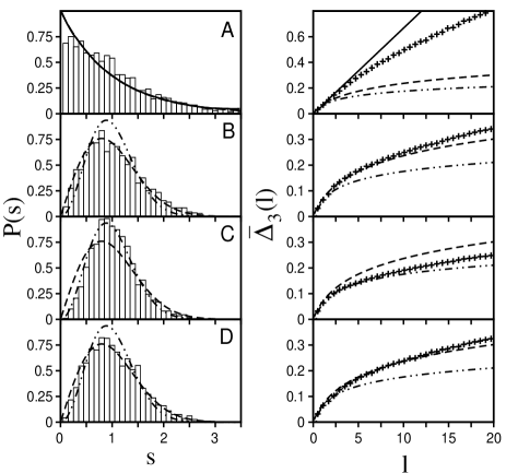
Figure 4: Energy-level statistics for the nanostructure with only the DP interaction, for $\beta_{DP}=10$ and four different positions (A,B,C, and D) for the center of the QD (refer to Fig. 3). The cavity boundary conditions are {FFFF}. The symbols $+$ represent the numerically calculated results. The curves indicate the expected behavior for regular (solid), chaotic GOE-type (dashed), and chaotic GUE-type (dot-dashed) systems.

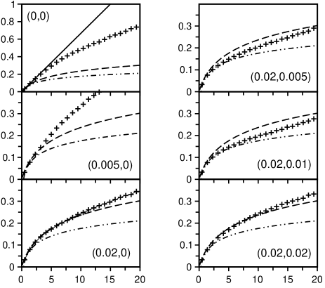
Figure 5: $\overline{\Delta}_{3}(l)\times l$ for different positions of the center of the circular QD. The cavity boundary conditions are {CCCC} and $\beta_{DP}=10$.

It is also instructive to look at the evolution of the spectral statistics as a function of the position of the QD. The effect is illustrated by the $\overline{\Delta}_{3}(l)$ statistics in Fig. 5, for the {CCCC} plate and the parameters of Fig. 4. Leaving A along the S_x axis the statistics evolves from regular to GOE, at (0.02,0), passing through a mixed behavior at the locus (0.005,0). Proceeding perpendicularly to the S_x axis, the statistics evolves from GOE towards GUE, (0.02,0) $\rightarrow$ (0.02,0.005) $\rightarrow$ (0.02,0.01) $\equiv$ C, going back to GOE when the S_x-y axis is reached at (0.02,0.02).

Table 1: Symmetry axes and spectral statistics for points A,B,C,D and E, as defined in the text, for a circular 2DEG. Here, 2 GOE means that the statistics can be described by the uncorrelated superposition of two GOE distributions.

Boundary Conditions	Symmetry axes	A	B	C	D	E
	for the phonon modes
{FFFF}	Sx, Sy, Sx-y, Sx+y	Regular	GOE	GUE	GOE	GOE
{CCCC}	Sx, Sy, Sx-y, Sx+y	Regular	GOE	GUE	GOE	GOE
{CCFF}	Sx, Sy	2 GOE	GUE	GUE	GOE	GOE
{CFCF}	Sx-y	GOE	GOE	GUE	GUE	GUE
{CCCF}	Sy	GOE	GUE	GUE	GUE	GOE
{CFFF}	Sx	GOE	GUE	GUE	GOE	GUE

By the examination of several different scenarios we were able to classify the general behavior of our system. Table I summarizes the results obtained for the center of the circular 2DEG located at points A,B,C,D and E with either the DP or the PZ interaction taken into account. Furthermore, we have considered a comprehensive set of boundary conditions, which are representative of all possible combinations of the Dirichlet and Neumann conditions for the phonon cavity, thus, producing distinct symmetry axes for the phonon modes: {CCCC}, {FFFF}, {CCFF}, {CFCF}, {CCCF}, and {CFFF}. From Table I, we see that the chaotic behavior is determined by the overall (or global) symmetries of the NEMS, that is, the one that results from the joint combination of the boundary conditions of the phonon cavity and the position of the QD. For instance, if the boundary conditions are {CCCC} and the QD is located at D, the S_y, S_x-y and S_x+y are not symmetry axes for the coupled electromechanical system. According to Table I, if the present NEMS has: (i) four symmetry axes (position A for {CCCC} and {FFFF} plates), the statistics indicates a regular (integrable) problem; (ii) two symmetry axes (position A for {CCFF}), then the statistics corresponds to the uncorrelated superposition of two distributions of the GOE type twowigner ; (iii) one symmetry axis, the results are those of GOE; and finally (iv) no symmetry axes at all, the spectrum exhibits the GUE statistics.

The boundary conditions determine not only the position of the center of the 2DEG at which regular, GOE or GUE statistics are obtained, but also the intensity of the quantum chaos. This happens because the electron-phonon coupling depends on the phonon energies, which vary according to the boundary conditions. The higher the phonon energy, the stronger the electron-phonon interaction, thus, leading to spectral fluctuations that are more faithful to the typical chaotic features. The energies of the phonon modes decrease according to the following sequence: {FFFF}, {CCFF}, {CCCC}, {CFFF}, {CCCF}, and {CFCF}. The energies for the first five boundary conditions are similar, and quantum chaos can be observed for essentially the same values of the interaction strength $\beta$. For the {CFCF} case, however, the phonon energies can be one order of magnitude smaller than the ones for the other cases, requiring larger values for the parameters $\beta_{DP}$ and $\beta_{PZ}$ (approximately 3 times larger).

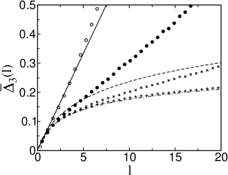
Figure 6: The calculated spectral rigidity for various DP coupling constants: $\beta_{DP}$=1 (open circle), 3 (filled circle), 5 ($\times$) and 10 ($+$). The system corresponds the {CCCC} plate with the QD located at position C. The curves represent the regular (solid), GOE (dashed) and GUE (dot-dashed) cases.

It is, however, important to notice that, regardless of the geometry adopted, the nanostructure shows a regular spectrum for the bare parameters of the reference materials. We present in Fig. 6 the dependence of the spectral rigidity $\overline{\Delta}_{3}(l)$ on the electron-phonon coupling strength. For the locus C of the {CCCC} phonon cavity, we take into account only the DP interaction, with $\beta_{DP}$ = 1, 3, 5, and 10. As $\beta$ increases, the calculated statistics gradually converges to the GUE prediction. Note that the numerical calculations are never well fitted by the GOE distribution. The inclusion of more basis states does not alter the observed results. At this point we observe that the strong el-ph coupling regime ($\beta>3$) can be achieved by using different materials. For instance, aluminum nitride (AlN) is a strong piezoelectric semiconductor, with $\varrho_{33}$=1.5 C/m², that is currently been used to produce nanomechanical resonators AlN . The piezoelectric constant for GaAs is $\varrho_{14}$=0.16 C/m²

Next, we summarize the effects of the geometrical and material parameters on the chaotic behavior. Irrespective of the boundary conditions, when the QD radius $R$ decreases to less than one third of the plate side $L$, the system starts to become regular and, for about $L/R\approx 5$, the nanostructure presents no clear signs of chaos in its spectrum. This is illustrated in the top panel of Fig. 7, by the $\overline{\Delta}_{3}(l)$ statistics calculated for case A in the {CFFF} plate. On the other hand, an important physical parameter for the occurrence of chaos is the in-plane electron effective mass $m^{*}$. It is shown in the bottom panel of Fig. 7 that chaos arises as $m^{*}/m_{e}$ is increased. Indeed, for $m^{*}\gtrsim 0.6$ the system is clearly chaotic, becoming regular for $m^{*}\lesssim 0.2\,m_{e}$. As before, similar results hold for other boundary conditions. A weak dependence on both the density and the value of the stiffness tensors $c_{12}$ and $c_{44}$ is also observed. In essence, lighter and softer materials favor the appearance of chaos. As for the size of the dielectric plate, chaos is favored by short and thin plates. The former should be expected because the phonon energies increase as the area of the plate decreases. However, structures much smaller than the one here considered do not present a significantly higher tendency to chaotic behavior.

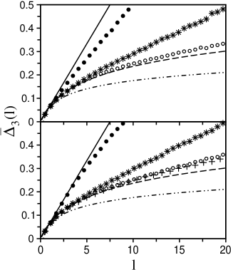
Figure 7: Top panel: $\overline{\Delta}_{3}(l)$ statistics at point A of the {CFFF} plate for various radii of the QD: $R$ = 200 nm (filled dot), 300 nm (star) and 400 nm (open dot); Bottom panel: same statistics for various $m^{*}/m_{e}$ ratios: 0.2 (filled dot), 0.4 (star), 0.6 (open dot), and 0.8 (cross). $\beta_{DP}$=10.

So far, we have considered only the DP or PZ interactions acting individually. When acting together, the spectrum statistics of loci B and D change from GOE to GUE. Fig. 8 demonstrates this effect by showing the $P(s)$ distribution for the circular QD at locus D in the {CCCC} plate, for both the DP and PZ interactions included with $\beta_{DP}=\beta_{PZ}=10$. The agreement with the GUE statistics is excellent, in contrast to case D of Fig. 4 (we recall that the {CCCC} and {FFFF} cases give similar results). Because the AlGaAs alloy is a weak piezoelectric material, the DP coupling shows a stronger effect in promoting the chaos, whereas the main action of the PZ interaction (in the presence of DP) is to break the system’s overall symmetry. The explanation for such a change in the spectrum statistics is left to Section V.

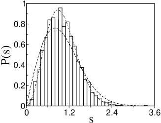
Figure 8: The nearest neighbor spacing distribution for the {CCCC} plate with the circular QD located at D. Both the DP and PZ interactions are included with $\beta_{DP}=\beta_{PZ}=10$. The curves correspond to GOE (dashed) and GUE (dot-dashed).

IV.2 Rectangular 2DEG

Table 2: The same as Table I, but for a rectangular quantum dot.

Boundary Conditions	Symmetry axes	A	B	C	D	E
	for the phonon modes
{FFFF}	Sx, Sy, Sx-y, Sx+y	Regular	2 GOE	GOE	2 GOE	2 GOE
{CCCC}	Sx, Sy, Sx-y, Sx+y	Regular	2 GOE	GOE	2 GOE	2 GOE
{CCFF}	Sx, Sy	Regular	GOE	GOE	2 GOE	2 GOE
{CFCF}	Sx-y	2 GOE	2 GOE	GOE	GOE	GOE
{CCCF}	Sy	2 GOE	GOE	GOE	GOE	2 GOE
{CFFF}	Sx	2 GOE	GOE	GOE	2 GOE	GOE

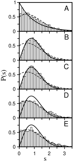
Figure 9: $P(s)$ for the {CCFF} boundary conditions and the rectangular QD centered at positions A, B, C, D, and E. Only the DP interaction is considered ($\beta_{DP}=10$). The dashed lines represent the uncorrelated superposition of two GOEs and the continuous lines the regular and GOE cases.

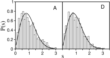
Figure 10: $P(s)$ for the {CFFF} boundary conditions and both interaction potentials acting together ($\beta_{DP}=\beta_{PZ}=10$). The rectangular QD is located at positions A (right panel) and D (left panel).

Chaos is also observed in the calculations for a rectangular 2DEG interacting with the suspended phonon cavity. In this section we investigate such nanostructures following the procedures previously described. The obtained statistics are summarized in Table II for the interactions, either DP or PZ, taking into account individually. The calculations were made for the same phonon cavity considered throughout Section IV.1, but now supporting a square QD of sides 400 nm and thickness equal to the circular case.

Representative results of the $P(s)$ distribution are shown in Fig.9, which illustrates the chaotic behavior of the {CCFF} phonon cavity through cases A to E. Here too, the global symmetries of the system depend on the combination of the symmetry axes of the plate with the position of the square QD. From extensive simulations we verified that (see Table II) whenever the full problem has only one global symmetry axis, either S_x, S_y, S_x-y or S_x+y, the resulting spectral statistics corresponds to the superposition of two uncorrelated GOEs, contrasting with the case of the circular QD-NEMS (see Table I). If there are no overall symmetry axes, the statistics is that of the GOE type. Finally, the spectrum is regular if there are at least two global symmetry axes, namely, the position A for the {CCFF}, {CCCC} or {FFFF} boundary conditions.

Despite the fact that circular and rectangular QD-NEMSs display chaotic features, it is important to emphasize that the GUE statistics never occurs for the rectangular 2DEG coupled to a rectangular phonon cavity. This is, therefore, an effect that results from the interplay between the cylindrical and rectangular symmetries in the circular QD-NEMS. We discuss this phenomenon in detail in the next Section.

The dependence of the spectrum statistics on the geometrical and material parameters is, nonetheless, similar to that observed for the circular QD. Specifically, heavier in-plane electron effective masses, lighter and softer materials and larger and thinner quantum dots favor the appearance of chaos. The {CFCF} plate requires stronger interaction strengths than the other boundary conditions to give rise to a chaotic spectrum.

Finally, when the system has one global symmetry axis and both the DP and PZ interactions act simultaneously, the spectrum statistics changes from two uncorrelated GOEs to a single GOE. This effect is illustrated in Fig 10 for the rectangular 2DEG centered at points A (right panel) and D (left panel) of the {CFFF} cavity. A comparison with Table II evidences the aforementioned transformation. On the other hand, when the nanostructure displays either regular or chaotic (GOE) distributions for one of the interactions, the inclusion of the other does not alter the original statistics, regardless of the strength of the interactions.

V Discussion

It has been shown that distinct geometrical configurations of the QD-NEMS produce different energy-level statistics, in most cases typical of chaotic dynamics. To understand this effect we investigate the structure of the Hamiltonian matrix of our systems and explain the previous results in terms of the underlying symmetries of the problem. At the end, we explain the anomalous GUE statistics in the light of a more general analysis Leyvraz ; Keating .

V.1 The Hamiltonian block structure due to the phonons

Figure 11: (a) A block of the interaction potential matrix representing fixed electron quantum numbers and all possible combinations for the phonon states. The small blocks $d$, shown in (b), are diagonal matrices whose diagonal elements $d_{ii}$ are all equal. The $t$’s forming the main diagonal in (a), depicted in (c), are also block tridiagonal matrices. Noticeably, d and t in (a) are different from the corresponding blocks in (c).

From the Eqs. (LABEL:DP) and (26), for the deformation and piezoelectric potentials, one verifies that the interaction mechanism is mediated by one phonon processes. This becomes clear by writing the matrix elements in the basis (29) [$\xi\equiv(\kappa,{\bf n})$]

$$h(\xi^{\prime\prime};\xi^{\prime}) = C\sqrt{\frac{\hbar}{2\rho V}}\sum_{\alpha}\frac{{\cal I}_{\alpha\,\kappa^{\prime\prime}\kappa^{\prime}}}{\sqrt{\omega_{\alpha}}}\,$$ (36)

$$\times\left[\delta_{n_{1}^{\prime\prime}\,n_{1}^{\prime}}\,\ldots\,\delta_{n_{\alpha}^{\prime\prime}\,n_{\alpha}^{\prime}-1}\,\ldots\delta_{n_{N}^{\prime\prime}\,n_{N}^{\prime}}\right.$$

$$+\left.\delta_{n_{1}^{\prime\prime}\,n_{1}^{\prime}}\,\ldots\,\delta_{n_{\alpha}^{\prime\prime}\,n_{\alpha}^{\prime}+1}\,\ldots\delta_{n_{N}^{\prime\prime}\,n_{N}^{\prime}}\right],$$

where $C$ and ${\cal I}_{\alpha\,\kappa^{\prime\prime}\kappa^{\prime}}$ denote, respectively, the appropriate coupling constant and the overlap of the phonon mode $\alpha$ with the electronic eigenfunctions $\kappa^{\prime\prime}$ and $\kappa^{\prime}$. Notice that the Kronecker $\delta$’s allow only a single phonon transition.

In this representation we have a very particular form for the interaction matrix. Consider the block ${\bf n}\times{\bf n}$, schematically depicted in Fig. 11 (a). It corresponds to fixed values for the electron quantum numbers $\kappa^{\prime\prime}$ and $\kappa^{\prime}$, but embraces all possible configurations for the phonon states. The structure of the block ${\bf n}\times{\bf n}$ is such that the outermost block spans all possible states for the phonon quantum number $n_{1}=0,1,\ldots,n$. Then, the next internal block spans the quantum number $n_{2}$, followed by the inner blocks $n_{3},n_{4}\,\ldots\,n_{N}$. Due to the action of the Kronecker $\delta$’s in (36), the ${\bf n}\times{\bf n}$ matrix is block tridiagonal. Consequently, the small blocks $d$ (refer to Fig. 11 (b)) must be diagonal, since the interactions are mediated by one phonon only. On the other hand, the small blocks $t$ are also tridiagonal (Fig. 11 (c)). Such self-similar arrangement goes on at all block levels $n_{1}\,n_{2}\,\ldots\,n_{N}$.

V.2 Phonon mode parities

The reflection symmetries of the phonon cavity lead to phonon modes of well defined parity. Such properties are examined in this section; for guidance refer to Fig. 3. For instance, when the boundary conditions at $Y_{1}$ and $Y_{2}$ are equal, i.e., both C or both F, the modes $\alpha$ have either a symmetric ($+$) or an anti-symmetric ($-$) parity with respect to S_x. The same holds for S_y regarding the edges $X_{1}$ and $X_{2}$. If the boundary conditions are opposite at $X_{1}$ and $X_{2}$ and also at $Y_{1}$ and $Y_{2}$, then one of the main diagonals of the plate, S_x-y or S_x+y, is the only symmetry axis. Therefore the phonon modes $\alpha$ have well defined $+$ and $-$ parities about it. Finally, the cases {CCCC} and {FFFF} have definite parities about all the symmetry axes: S_x, S_y, S_x-y and S_x+y.

V.3 Circular quantum dot

In the following we analyze the element ${\cal I}_{\alpha\,\kappa^{\prime\prime}\kappa^{\prime}}$, appearing in Eq. (36). For the circular quantum dot case we have, generalizing Eqs. (21) and (27),

$${\cal I}_{\alpha\,\kappa^{\prime\prime}\kappa^{\prime}} = f(d)\int_{\mathcal{D}_{xy}}dx\,dy\ \ g_{\kappa^{\prime\prime}\kappa^{\prime}}(r)\ \ F_{\alpha}(x,y)$$ (37)

$$\times \big{\{}\cos[(l^{\prime\prime}-l^{\prime})\,\theta]+i\sin[(l^{\prime\prime}-l^{\prime})\,\theta]\big{\}}.$$

Here, $g_{\kappa^{\prime\prime}\kappa^{\prime}}(r)$ denotes the product of Bessel functions coming from Eq. (16), $r=\sqrt{(x-x_{0})^{2}+(y-y_{0})^{2}}$ with $(x_{0},y_{0})$ as the center of the QD, $\theta$ is measured from the S_x axis and $f(d)$ results from a simple integration along the $z$ axis. For the deformation potential $F_{\alpha}^{DP}(x,y)=\nabla^{2}\sum_{m,n}A_{mn}^{\alpha}\,X_{m}(x)\,Y_{n}(y)$, whereas for the piezoelectric interaction $F_{\alpha}^{PZ}(x,y)=\frac{\partial^{2}}{\partial x\,\partial y}\sum_{m,n}A_{mn}^{\alpha}\,X_{m}(x)\,Y_{n}(y)$. Notice that the Laplacian is a second order operator, therefore the function $F_{\alpha}^{DP}$ has the same parity as the phonon mode $\alpha$. On the other hand, $F_{\alpha}^{PZ}$ results from first order derivatives, so it has the opposite parity of $\alpha$.

Figure 12: Circular quantum dot positioned at: (a) locus A for the {FCCC} (or {CFFF}) plate; and (b) locus D for the {$X_{1}X_{2}$CC} (or {$X_{1}X_{2}$FF}) plate. Notice that both cases have overall symmetry only about the $x$ axis, i.e., S_x.

A first examination of Eq. (37) reveals that if $l^{\prime\prime}=l^{\prime}$ the sine function vanishes and the matrix element is real. For $l^{\prime\prime}\neq l^{\prime}$, it will be complex, real or purely imaginary depending on the system’s characteristics. For the sake of understanding we shall briefly analyze a representative case. Let us assume the same boundary conditions for $Y_{1}$ and $Y_{2}$, then consider two scenarios: the circular QD at locus A and different boundary conditions for $X_{1}$ and $X_{2}$ (Fig. 12(a)), or locus D regardless of $X_{1}$ and $X_{2}$ (Fig 12(b)). In both cases only the phonon parity about the S_x axis will be relevant for the evaluation of (37). In fact, the $+$ ($-$) parity of $F_{\alpha}$ about S_x leads to a matrix element that is real (purely imaginary) for the DP interaction and purely imaginary (real) for the PZ interaction. That is a consequence of the parity of the sine and cosine functions about $\theta=0$ together with the parity of $F_{\alpha}$ regarding the same axis.

On the basis of the above analysis and the discussion of Section V.1, it follows that if there is one or more global symmetry axes in the system, then each matrix block ${\bf n}\times{\bf n}$ of Fig. 11(a) can be written as $\mathbb{A}+i\mathbb{B}$, with $\mathbb{A}$ and $\mathbb{B}$ originating from the cosine and sine parts of the integral in Eq. (37), respectively. Moreover, those matrices are real symmetric and mutually disjoint, that is, for $\mathbb{A}_{rs}\neq 0$ ($\mathbb{B}_{rs}\neq 0$) necessarily $\mathbb{B}_{rs}=0$ ($\mathbb{A}_{rs}=0$).

Therefore, when a single interaction mechanisms is acting, we have the following scenarios:

• If the geometrical configuration of the nanostructure is such that there is only one global symmetry axis (e.g., locus A or D for plate {CFFF}), the ensuing partial symmetry break is enough to generate chaos. Moreover, the matrix representation of the Hamiltonian $\hat{H}=\hat{H}_{0}+\hat{H}_{DP(PZ)}$ can be written in blocks of fixed $l$’s as $\mathbb{H}_{l^{\prime\prime}l^{\prime}}=\mathbb{A}_{l^{\prime\prime}l^{\prime}}+(i)^{\mbox{\scriptsize{sign}}(l^{\prime\prime}-l^{\prime})}\,\mathbb{B}_{l^{\prime\prime}l^{\prime}}$, where $\mathbb{A}$ and $\mathbb{B}$ are disjoint, real and symmetric. Thus, $\mathbb{H}$ is completely characterized by orthogonal matrices, so belonging to the GOE universality class. It is straightforward to verify that the present reasoning encompasses all the cases of a single GOE statistics listed in Table I.

• For locus A and {CCFF} boundary conditions, the above structure for $\mathbb{H}$ is still valid. However, now the system has two symmetry axes, leading to new restrictions for the matrix elements. In fact, denote by $\sigma_{x}\sigma_{y}$ (with $\sigma=\pm$) the $\alpha$ mode parities with respect to S_x and S_y. One finds that the integral over the cosine (sine) in Eq. (37) is different from zero only if $|l^{\prime\prime}-l^{\prime}|$ is even and the $\alpha$ mode is $++$ ($--$), or $|l^{\prime\prime}-l^{\prime}|$ is odd and the $\alpha$ mode is $+-$ ($-+$). Such selection rules produce two different families of eigenvalues for the problem. For {CCFF} (and {FFCC}) each distinct family is chaotic, explaining the occurrence of two superposed uncorrelated Wigner distributions in the $P(s)$ statistics (for an explicit example, see the simpler case of a rectangular QD in Sec. V-D).

• For locus A and boundary conditions {CCCC} (or {FFFF}) there exists one further global symmetry, namely, the equivalence of the $x$ and $y$ directions. The extra symmetry prevents the emergence of chaos.

• Finally, in the absence of a global symmetry axis (e.g., the quantum dot at C for any boundary condition, or loci B, C or E for {CFFF}) the Hamiltonian matrix does not separate into real and purely imaginary disjoint parts. Hence, it is a full complex unitary matrix and the chaotic behavior takes place with the system belonging to the GUE universality class.

The last case to be considered is the inclusion of both interactions in the Hamiltonian. From the previous discussion we know that for a given parity of the mode $\alpha$ the DP and PZ potentials lead to exactly opposite types of matrix elements. Indeed, if the DP matrix element is real (pure imaginary), necessarily that corresponding to PZ is pure imaginary (real). Therefore, the Hamiltonian $\hat{H}=\hat{H}_{0}+\hat{H}_{DP}+\hat{H}_{PZ}$ has a complex matrix representation that results in a GUE statistics for the energy levels.

V.4 Rectangular quantum dot

Figure 13: Top: schematics of the $32\times 32$ interaction matrix for locus D in the {CCFF} nanostructure, ordered as $p\,q\,\alpha_{1}\,\alpha_{2}\,\alpha_{3}$ with $p,q=1\ \mbox{or}\ 2$ and $\alpha_{j}=0\ \mbox{or}\ 1$. Bottom: the transformed matrix in a block form. The filled dots indicate the nonzero elements.

For the rectangular quantum dot the element ${\cal I}_{\alpha\,\kappa^{\prime\prime}\kappa^{\prime}}$ can be written as

$${\cal I}_{\alpha\,\kappa^{\prime\prime}\kappa^{\prime}} = f(d)\int_{\mathcal{D}_{xy}}dx\,dy\,F_{\alpha}(x,y)$$ (38)

$$\sin[p^{\prime\prime}\pi\frac{(x-\overline{x})}{L_{x}}]\,\sin[q^{\prime\prime}\pi\frac{(y-\overline{y})}{L_{y}}]$$

$$\times\sin[p^{\prime}\pi\frac{(x-\overline{x})}{L_{x}}]\,\sin[q^{\prime}\pi\frac{(y-\overline{y})}{L_{y}}],$$

where $\overline{x}=x_{0}-L_{x}/2$, $\overline{y}=y_{0}-L_{y}/2$ and $(x_{0},y_{0})$ are the coordinates of the center of the QD (for guidance refer to Section II.2). From Eq. (38) it is evident that the matrix elements are always real numbers. Consequently, any chaotic behavior must belong to the GOE class and the occurrence of the GUE statistics is ruled out for this nanostructure.

With respect to the quantum numbers, the conditions for which the above integral is different from zero are again entirely dependent on the global symmetries of the system. For instance, if the whole nanostructure has S_x as a symmetry axis, then ${\cal I}_{\alpha\,\kappa^{\prime\prime}\kappa^{\prime}}$ is nonzero for the following combinations: $p^{\prime\prime}+p^{\prime}\equiv$ even and $\alpha$ mode parity $\sigma_{x}\equiv+$, or $p^{\prime\prime}+p^{\prime}\equiv$ odd and $\sigma_{x}\equiv-$. Similar relations hold for $q^{\prime\prime}+q^{\prime}$ regarding S_y.

The behavior of the spectral statistics generated by the rectangular QD-NEMS can be summarized by the following representative situations: for the loci B, C or E in the {CFFF} plate there are no global symmetry axes and we obtain GOE distributions. For loci A and D in the {CFFF} plate, there is one overall symmetry axis (S_x) and the resultant statistics is the superposition of two uncorrelated GOE distributions. Finally, for locus A in the {CCFF} and {FFFF} (or {CCCC}) plates, which contain more than one global symmetry axes, no chaotic features are observed. One can verify that all cases in Table II follow the same trends.

In order to visualize the occurrence of the 2-GOE statistics, consider the case D in the {CCFF} plate. Despite the fact that the phonon modes $\alpha$ have two symmetry axes, S_x and S_y, only the parity about S_x is a global symmetry, due to the position of the QD. Assume then 3 phonon modes, such that a basis state is written as $|p,q;n_{1},n_{2},n_{3}\rangle$, with $p,q$=1 or 2 and $n_{\alpha}$=0 or 1. In addition, the 3 phonon mode parities with respect to S_x are taken to be {$+,-,+$}. It results in the $32\times 32$ matrix schematically represented in the top of Fig. 13, where the filled dots indicate the nonzero elements. It is possible to transform the original matrix in that shown at the bottom of Fig. 13 just by rearranging its rows and columns. By labelling the original rows (from left to right) and columns (from top to bottom) as $1,2,\ldots,32$, we obtain the first nonzero block of the transformed matrix by performing the operation $1\,2\,3\,4\,5\,6\,7\,8\,9\,10\,11\,12\,13\,14\,15\,16\rightarrow 1\,2\,5\,27\,13\,19\,10\,9\,32\,31\,6\,20\,14\,28\,23\,24$. A similar procedure, i.e., operating over the remaining $17\ldots 32$ positions, leads to the other nonzero block. Here, the el-ph interaction generates chaos in each family of eigenvalues, originating from the two independent blocks. Consequently, the spectrum of the full matrix gives rise to the superposition of two uncorrelated GOE distributions. The above analysis is valid for any matrix size.

Finally, if both interactions act together in a system with a single global symmetry axis, say S_x, their effect is to break the selection rules previously described. This happens because $F_{\alpha}(x,y)$ has opposite parities for the DP and PZ interactions. As a result the Hamiltonian matrix does not have a block form and a pure GOE statistics emerges from the 2-GOE case, as seen in Fig. 10.

V.5 Symmetry operator analysis of the anomalous GUE statistics

So far we have examined the structure of the Hamiltonian matrix to explain the chaotic features exhibited by our NEMS. Here, we make a link between our results and a more general analysis Leyvraz to clarify the appearance of the anomalous GUE statistics in our time-reversal invariant (TRI) system.

As already mentioned, the spectral fluctuations of TRI chaotic systems typically correspond to the GOE distribution. However, Leyvraz et al. Leyvraz have shown that there are exceptions to this rule, which can be interpreted even semiclassically Keating . Suppose a TRI chaotic system that has a discrete point symmetry represented by the operator ${\cal S}$, then $[H,{\cal S}]=[H,{\cal T}]=0$, where $H$ is the Hamiltonian and ${\cal T}$ the time reversal operator. More importantly for the effect, assume also that ${\cal S}$ has two invariant subspaces whose representations are complex conjugate of each other. We call them $\{\Psi^{(+)}\}$ and $\{\Psi^{(-)}\}$, which are solutions of $H\Psi_{n}^{(\pm)}=E_{n}^{(\pm)}\Psi_{n}^{(\pm)}$. Since ${\cal T}\Psi_{n}^{(\pm)}=[{\Psi_{n}^{(\pm)}}]^{*}=\Psi_{n}^{(\mp)}$, it may seem that the problem is not TRI because each subspace changes into the other under ${\cal T}$, therefore causing a GUE statistics (notice that the Hamiltonian matrix is complex Hermitian in this basis). However, this is just an artefact of the particular structure of the subspaces. Actually, the full Hilbert space is TRI, as can be verified after the simple basis transformation $\Phi^{(\pm)}=i^{(\pm 1-1)/2}[\Psi^{(+)}\pm\Psi^{(-)}]/\sqrt{2}$, for which ${\cal T}\Phi_{n}^{(\pm)}={\Phi_{n}^{(\pm)}}$. Note also that the Kramers theorem Sakurai ; Dembowski2 imposes $E_{n}^{(+)}=E_{n}^{(-)}$. Finally, as pointed out in Ref. [Leyvraz, ], the present phenomenon is rare because often there exists an extra operator ${\cal P}$ (e.g., the parity symmetry operator) for which $[H,{\cal P}]=[{\cal T},{\cal P}]=0$. This operator is responsible for combining the two complex conjugate representations of ${\cal S}$ into an irreducible representation that is self-conjugate Schafer , therefore producing a GOE statistics.

Prior to our earliest paper rego , the only systems known to show such behavior were billiards with three-fold but no mirror (parity) symmetries, which have been realized experimentally in microwave cavities Schafer ; Dembowski1 ; Dembowski2 . They are chaotic by construction (due to their particular geometry) and have their eigenstates composed by complex degenerate doublets (of GUE statistics) and real singlets (of GOE statistics). It is possible, however, to establish a parallel between our circular QD-NEMS and these billiards. In our case the electron states, Eq. (16), naturally provide the necessary complex representation through the angular momentum quantum number $l$. They are divided in singlets, for $l=0$, and degenerate doublets, for $l=\pm 1,\pm 2,\ldots$. Of course, the original electron states as well as the phonon states are regular, but the el-ph coupling generates chaos. If, nevertheless, the boundary conditions and the location of the QD are such to give rise to an global symmetry axis, the energy-level statistics is of the GOE type due to the ensuing definite parity. On the other hand, in the absence of an overall symmetry axis (e.g., location C for any plate), no ${\cal P}$ operator exists and GUE statistics arises.

As a last comment, we recall that in our system the original electron degeneracies are destroyed by the interaction with the phonons. Nonetheless, the last behave as a perturbation for the electronic spectrum, because the energies of the electrons are much higher than those for an individual phonon. It is important to mention, however, that the occurrence of the doublets is not necessary for the manifestation of the GUE statistics. Actually, even when an additional small perturbation breaks that degeneracy, the GUE statistics also arises for each split family of eigenstates. It has been confirmed experimentally by the study of imperfect three-fold microwave triangular billiards Dembowski1 .

VI Conclusion

We have presented a theoretical study of the electron-phonon coupling in nanoelectromechanical systems (NEMS) comprised of a suspended dielectric plate and a quantum dot on its surface. It is shown that a quantum chaotic behavior develops as a result of the el-ph interaction, for a wide range of geometrical and material parameters of the QD-NEMS. A method is developed to treat this novel class of systems. It associates the phonons with the vibrational modes of a suspended rectangular plate, for clamped and free boundary conditions. The electrons are confined to a large QD, of either circular or rectangular symmetry, and described by the free electron gas approximation. The deformation potential and piezoelectric interactions are included non-perturbatively in the model, by calculating the eigenenergies of the NEMS on the basis of the el-ph states.

By performing standard energy-level statistics we demonstrate that the resulting spectral fluctuations are very well described by those of the Gaussian Orthogonal Ensemble (GOE) or the Gaussian Unitary Ensemble (GUE). It is evidenced that the combination of the phonon mode parities together with the position of the QD determine the overall symmetries of the system, which are ultimately the responsible for the distinct chaotic features observed. Although, quantum chaos is commonly obtained in the system, the GUE statistics occurs only in the case of a circular QD-NEMS. It represents an anomalous phenomenon, since the problem is time-reversal invariant. The fundamental reason for this effect lies in the structure of the electronic spectrum, which is formed by doublets with $l=\pm 1,\pm 2,\ldots$. In the absence of any overall geometrical symmetry, the complex conjugate doublets transform into each other under the action of the time reversal operator, thus simulating the behavior of a non-TRI system.

Finally, calculations are under way to include the effects of the electron-electron interaction in the model. We conjecture that the same chaotic behavior can also arise in this case, because the el-el interaction preserves the total angular momentum of the electronic system, justifying the previous analysis.

References

- (1) T. Brandes, Phys. Rep. 408, 315 (2005).
- (2) H. Bruus and A. D. Stone, Phys. Rev. B 50, 18275 (1994).
- (3) K.-F. Berggren and Z.-L. Ji, Chaos 6, 543 (1996).
- (4) C. W. J. Beenakker, Rev. Mod. Phys. 69, 731 (1997).
- (5) H. J. Stockmann, Quantum Chaos: an Introduction (Cambridge Univ. Press, UK, 1999).
- (6) C. M. Marcus, A. J. Rimberg, R. M. Westervelt, P. F. Hopkins, and A. C. Gossard, Phys. Rev. Lett. 69, 506 (1992).
- (7) T. M. Fromhold, P. B. Wilkinson, F. W. Sheard, L. Eaves, J. Miao, and G. Edwards, Phys. Rev. Lett. 75, 1142 (1995).
- (8) E. J. Heller, Phys. Rev. Lett. 53, 1515 (1984).
- (9) M. F. Crommie, C. P. Lutz, D. M. Eigler, and E. J. Heller, Physica D 83, 98 (1995).
- (10) D. A. Magder, F. Simmel, D. A. Wharam, M. A. Kastner, and J. P. Kotthaus, Physica E 6, 382 (2000).
- (11) A. N. Cleland, Foundations of Nanomechanics (Springer-Verlag, 2002); R. H. Blick, A. Erbe, L. Pescini, A. Kraus, D. V. Scheible, F. W. Beil, E. Hoehberger, A. Hoerner, J. Kirschbaum, and H. Lorenz, J. Phys.: Cond. Matt. 14, R905 (2002).
- (12) A. D. Armour, M. P. Blencowe, and K. C. Schwab, Phys. Rev. Lett. 88, 148301 (2002).
- (13) I. L. Chuang, R. Laflamme, P. W. Shor, and W. H. Zurek, Science 270, 1633 (1995).
- (14) A. N. Cleland and M. R. Geller, Phys. Rev. Lett. 93, 070501 (2004).
- (15) B. Georgeot and D. L. Shepelyansky, Phys. Rev. E 62, 3504 (2000); ibid, 6366 (2000).
- (16) L. G. C. Rego, A. Gusso, and M. G. E. da Luz J. Phys. A 38, L639 (2005).
- (17) M. L. Mehta, Random Matrices (Academic, New York, 1991).
- (18) D. V. Anghel, J. P. Pekola, M. M. Leivo, J. K. Suoknuuti, and M. Manninen, Phys. Rev. Lett. 81, 2958 (1998).
- (19) Karl A. Graff, Wave Motion in Elastic Solids (Dover, NY, 1975).
- (20) G. F. Elsbernd and A. W. Leissa, Developments in Theoretical and Applied Mechanics, 19-28 (1970).
- (21) To achieve the orthonormalization condition for the one-dimensional modes with the Multiprecision package MPFUN was used to calculate the wave vectors with a 200 digit precision.
- (22) B. A. Auld, Acoustic Fields and Waves in Solids (Krieger Publishing, Florida, 1990).
- (23) M. C. Guztwiller, Chaos in Classical and Quantum Mechanics (Springer-Verlag, New York, 1990).
- (24) T. Guhr, A. M. Groeling, and H. A. Weidenmuller, Phys. Rep. 299, 189 (1998).
- (25) A. G. Miltenburg and Th. W. Ruijgrok, Physica A 210, 476 (1994).
- (26) M. Van Vessen Jr., M. C. Santos, B. K. Cheng, and M. G. E. da Luz, Phys. Rev. E 64, 026210 (2001); E. P. S. Xavier, M. C. Santos, L. G. G. V. Dias, M. G. E. da Luz, M. W. Beims; Physica A 342, 377 (2004).
- (27) O. Bohigas, M. J. Giannoni, and C. Schmit, Phys. Rev. Lett. 52, 1 (1984).
- (28) F. Leyvraz, C. Schmit, and H. Seligman, J. Phys. A, 29, L575 (1996).
- (29) J. P. Keating and J. M. Robbins, J. Phys. A, 30, L177 (1997).
- (30) C. Dembowski, H.-D. Gräff, A. Heine, H. Rehfeld, A. Richter, and C. Schmidt, Phys. Rev. E 62, R4516 (2000)
- (31) C. Dembowski, B. Dietz, H.-D. Gräff, A. Heine, F. Levyraz, M. M.-Oglu, A. Richter, and T. Seligman, Phys. Rev. Lett. 90, 014102 (2003).
- (32) R. Schäfer, M. Barth, F. Levyraz, M. Müller, T. H. Seligman, and H. J. Stockmann, Phys. Rev. E 66, 016202 (2002).
- (33) S. Adachi, J. Appl. Phys. 58, R1 (1985).
- (34) T. Guhr and H. A. Weidenmüller, Ann. Phys. (N.Y.) 199, 412 (1990); C. Ellegaard, T. Guhr, K. Lindemann, J. Nygard, and M. Oxborrow, Phys. Rev. Lett. 77, 4918 (1996); M. S. Hussein, C. P. Malta, M. P. Pato, and A. P. B. Tufaile, Phys. Rev. E 65, 057203 (2002).
- (35) A. N. Cleland, M. Pophristic, and I. Ferguson, Appl. Phys. Lett. 79, 2070 (2001).
- (36) J. J. Sakurai, Modern Quantum Mechanics (Addison Wesley, Reading MA, 1985).