Quantum critical dynamics of the two-dimensional Bose gas

Abstract

The dilute, two-dimensional Bose gas exhibits a novel regime of relaxational dynamics in the regime $k_{B}T\gtrsim|\mu|$ where $T$ is the absolute temperature and $\mu$ is the chemical potential. This may also be interpreted as the quantum criticality of the zero density quantum critical point at $\mu=0$. We present a theory for this dynamics, to leading order in $1/\ln(\Lambda/(k_{B}T))$, where $\Lambda$ is a high energy cutoff. Although pairwise interactions between the bosons are weak at low energy scales, the collective dynamics are strongly coupled even when $\ln(\Lambda/T)$ is large. We argue that the strong-coupling effects can be isolated in an effective classical model, which is then solved numerically. Applications to experiments on the gap-closing transition of spin gap antiferromagnets in an applied field are presented.

I Introduction

Despite the widespread recent theoretical and experimental interest in quantum phase transitions, a direct quantitative confrontation between theory and experiment has been difficult to achieve for systems in two and higher spatial dimensions. A major obstacle is that it is often difficult to tune system parameters over the range necessary to move across a quantum critical point. Furthermore, for many examples where such tuning is possible, the theory for the quantum critical point is intractable. Consequently, the analysis of the data is often limited to the testing of general scaling ansatzes, without specific quantitative theoretical predictions.

A class of quantum phase transitions have recently been exceptionally well characterized in a variety of experiments. These experiments study the influence of a strong applied magnetic field on insulating spin-gap compoundsoosawa ; sebastian ; zapf ; stone ; stone2 ; hong . The low lying spin excitations behave like spin $S_{z}=1$ canonical Bose particles, and the energy required to create these bosons vanishes at a critical field $H=H_{c}$, which signals the position of a quantum phase transitionsss with dynamic critical exponent $z=2$. In spatial dimensions $d=3$, the quantum critical fluctuations are well described by the familiar Bose-Einstein theory of non-interacting bosons, and no sophisticated theory of quantum criticality is therefore necessary to interpret the experiments. The upper-critical dimension of the quantum critical point is $d=2$, and the boson-boson interaction vanishes logarithmically at low momenta. So naively, one expects that the $d=2$ case is also weakly coupled, and no non-trivial quantum critical behavior obtains.

The primary purpose of this paper is to show that the above expectation for the quantum-criticality of $d=2$ Bose gas is incorrect. While the pairwise interactions between the bosons are indeed weak, the collective properties of the finite-density, thermally excited Bose gas pose a strong-coupling problem. We will demonstrate here that an effective classical model, which can be readily numerically simulated, provides a controlled description of this problem. This will allow us to present predictions for the evolution of the dynamic spectrum of the $d=2$ Bose gas across the quantum critical point at non-zero temperatures.

Our results can be applied to two-dimensional spin-gap antiferromagnets, in the vicinity of the gap-closing transition induced by an applied magnetic. Recent experimentsstone ; stone2 ; hong on piperazinium hexachlorodicuprate (PHCC), (C₄H₁₂N₂)Cu₂Cl₆, will be compared with our results in Section III. These experiments are able to easily access the finite temperature quantum-critical region, which we will describe by our theory of the dilute Bose gas in $d=2$; this Bose gas is in a regime of parameters which is typically not examined in the context of more conventional atomic Bose gas systems popov ; fisher .

Results similar to those presented here ashvin also apply to other quantum critical points with upper-critical spatial dimension $d=2$ i.e. while the zero temperature properties can be described in a weak-coupling theory, all non-zero temperature observables require solution of a strong-coupling problem. A prominent example of such a quantum-critical point is the Hertz theory of the onset of spin-density-wave order in a Fermi liquidhertz . Results for the thermodynamic and transport properties can be obtained by the methods presented here ashvin . We maintain that such results are necessary for understanding experiments, and that previous theoretical resultshertz ; moriya ; millis are inadequate for a quantitative analysis.

Our results will be presented in the context of the phase diagram of the $d=2$ Bose gas shown in Fig. 1 as a function of the boson chemical potential, $\mu$, and temperature, $T$.

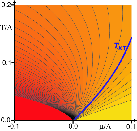
Figure 1: Color density plot of the value of the dimensionless ratio $U/R$ as a function of the chemical potential $\mu$ and the temperature $T$ of a dilute Bose gas in two spatial dimensions. The energy scale $U$, defined in Eq. (3), is a measure of the pairwise interaction between the atoms, while $R$, defined in Eq. (4), is an energy scale controlling collective excitations. The physical properties of systems with the same value of $U/R$ are the same, apart from the change in the value of the energy scale $R$. The Kosterlitz-Thouless transition occurs at the contour labelled $T_{KT}$ at ss1 ; nikolay1 $U/R\approx 34$, and the superfluid phase is present for larger $U/R$. The contours shown are for equal spacings of values of $R/U$, with the yellow region on the lower right including values $R/U\rightarrow 0$. Our primary results here are in the quantum critical region, with intermediate values of $U/R$ at $\mu=0$ and $T>0$.

At $T=0$, there is a quantum critical point at $\mu=0$. For $\mu<0$, the ground state is simply the vacuum with no bosons, while for $\mu>0$, there is a finite density of bosons in the ground state. In the spin gap antiferromagnets, $\mu=g\mu_{B}(H-H_{c})$, where $H$ is the applied field, $H_{c}$ is the critical field, $g$ is the gyromagnetic ratio, and $\mu_{B}$ is the Bohr magneton.

Fig. 1 presents results in terms of contours with equivalent physical properties, up to an overall energy scale ($R$) whose $T$ and $\mu$ dependence will be explicitly presented below, as will the equations determining the shape of the contours. One of the contours is the position of the Kosterlitz-Thouless (KT) transition of the $d=2$ Bose gas, which is present only for $\mu>0$. We are primarily interested here in the quantum-critical region,sss which is roughly the region with $k_{B}T\gtrsim|\mu|$. In particular, we will be able to quantitatively examine the signature relaxation rate $\sim k_{B}T/\hbar$ of the quantum-critical regimes: the “Bose molasses” dynamics. Our results and methods also describe the crossover to the KT transition, as well as (in principle) the region with $T<T_{\rm KT}$.

I.1 Summary of results

We summarize here the universal aspects of our results of the quantum-critical Bose dynamics in two spatial dimensions. The continuum quantum field theory of the critical point has logarithmic corrections to scaling; consequently, the properties of the continuum theory do have a logarithmic dependence upon a non-universal ultraviolet cutoff. We will show that this cutoff dependence can be isolated within a single parameter; all other aspects of the theory remain universal, and can be accurately computed.

We will be interested in the continuum Bose gas theory with the partition function

$$\mathcal{Z}_{B} = \int\mathcal{D}\psi({\bf r},\tau)e^{-\mathcal{S}_{B}/\hbar}$$

$$\mathcal{S}_{B} = \int_{0}^{\hbar/k_{B}T}d\tau\int d^{2}r\Biggl{[}\hbar\psi^{\ast}\frac{\partial\psi}{\partial\tau}+\frac{\hbar^{2}}{2m}\left|\nabla_{\bf r}\psi\right|^{2}-\mu|\psi|^{2}$$ (1)

$$~{}~{}~{}~{}~{}~{}~{}~{}~{}~{}~{}~{}~{}~{}~{}~{}~{}~{}~{}~{}~{}~{}~{}+\frac{V_{0}}{2}|\psi|^{4}\Biggr{]}.$$

For PHCC, the mass $m$ can be directly determined from the dispersion of the $S_{z}=1$ excitation. We will present results primarily in the small $|\mu|$ quantum critical region of Fig 1, although our formalism can be extended to other regions, including across the Kosterlitz-Thouless transition into the “superfluid” phase. The bare interaction between the Bose particles, $V_{0}$, is renormalized by repeated interactions between the particles, in the $T$ matrix, to the value

$$V_{R}=\frac{4\pi\hbar^{2}}{m\ln(\Lambda/\sqrt{\mu^{2}+(k_{B}T)^{2}})},$$ (2)

where $\Lambda$ is a high energy cutoff, and the square-root function in the argument of the logarithm is an arbitrary, convenient interpolating form. The parameter $\Lambda$ is the sole non-universal parameter appearing in the predictions of the continuum theory. For a spin gap antiferromagnet like PHCC, we expect $\Lambda\sim J$, where $J$ is a typical exchange constant. For our purposes, it is convenient to rescale $V_{R}$ to a parameter $U$, which has the dimensions of energy:

$$U\equiv\frac{2mk_{B}T}{\hbar^{2}}V_{R}=\frac{8\pi k_{B}T}{(\Lambda/\sqrt{\mu^{2}+(k_{B}T)^{2}})}.$$ (3)

Our universal results for the continuum theory are predicated on the assumption that the logarithm in Eqs. (2) and (3) is “large”. At first glance, it would appear from Eq. (2) that the quantum theory of the Bose gas is weakly coupled in the leading-logarithm approximation. However, as will be clear from our analysis (and has been noted in earlier works ss1 ; nikolay1 ; nikolay2 ; phase ), this is not the case: although pairwise interactions are weak, the collective static and dynamic properties of the gas remain strongly coupled even when the logarithm is large. We shall argue, that to leading order in the logarithm, these strong coupling effects can be captured in an effective classical model. The latter model is amenable to straightforward numerical simulations, and so accurate quantitative predictions become possible, whose precision is limited only by the available computer time. Previous analyses popov ; fisher ; dp of the dilute Bose gas in two dimensions assumed (when extended to the quantum critical region) that $\ln\ln(\Lambda/(k_{B}T))$ was large; a more precise version of this condition appears below, from which it is clear that this condition is essentially impossible to satisfy in practice. We will not make any assumption on the value of such a double logarithm, and only make the much less restrictive assumption on a large single logarithm.

The characteristic length and time scales of the quantum-critical Bose gas are set by a dimensionful parameter, which we denote $R$. Like $U$, we choose this to have dimensions of energy; so a characteristic length is $\hbar/\sqrt{2mR}$, while a characteristic time is $\hbar/R$. The value of $R$ is determined by the solution of the following equation

$$R=-\mu+\frac{U}{2\pi}\ln\left(\frac{\mu}{(e^{\mu/k_{B}T}-1)R}\right).$$ (4)

Note that this defines a $R>0$ for all $-\infty<\mu<\infty$.

To understand the magnitude of the various scales, we now discuss approximate solutions of Eqs. (3) and (4) at the quantum critical point, $\mu=0$. The estimates below should not be used in place of the full solutions in applications of our results to experiments. For the energy scale associated with $R$ we obtain the estimate

$$R\sim k_{B}T\frac{4\ln\left(\frac{1}{4}\ln(\Lambda/(k_{B}T))\right)}{\ln(\Lambda/(k_{B}T))}~{}~{}~{};~{}~{}~{}\mu=0.$$ (5)

Note that the energy scale $R$ is logarithmically smaller than $k_{B}T$: this will be the key in justifying an effective classical description of the dynamics. Numerically, we can easily go beyond Eq. (5), and obtain the full solution of Eq. (4) at $\mu=0$; this is shown in Fig. 2.

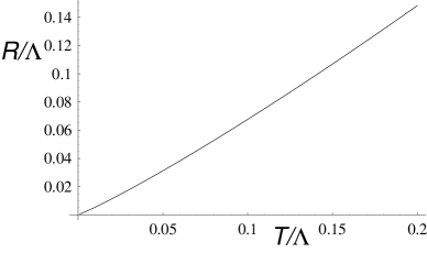
Figure 2: $T$ dependence of $R$ at the quantum critical point, $\mu=0$, obtained by solving Eq. (4). $\Lambda$ is a non-universal ultraviolet energy cutoff.

With the two dimensionful parameters, $U$, and $R$, at hand, the reader will not be surprised to learn that the effective classical theory is characterized by the dimensionless coupling $U/R$. Indeed, as we will see, the ratio $U/R$ behaves like an effective Ginzburg parameter for the classical theory. From Eqs. (4) and (5) we estimate

$$\frac{U}{R}\sim\frac{2\pi}{\ln\left(\frac{1}{4}\ln(\Lambda/(k_{B}T))\right)}~{}~{}~{};~{}~{}~{}\mu=0,$$ (6)

in the quantum-critical region. Again, we can go beyond the asymptotics, and obtain precise values for $U/R$ by numerical solution of Eqs. (4) and (3), and the result appears in Fig 3.

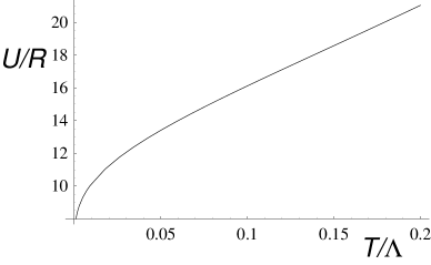
Figure 3: $T$ dependence of the dimensionless ratio $U/R$ at the quantum critical point, $\mu=0$.

So, unless $\Lambda/(k_{B}T)$ is astronomically large, the ratio $U/R$ is not small, and the classical theory is strongly coupled. As we have already noted, we will not make the assumption of large double logarithms here, but instead obtain numerical results for the strongly coupled theory.

The primary result of this paper is that the low energy properties of the dilute Bose gas are universal functions of the ratio $U/R$. This key result is illustrated in Fig 1 where we plot the loci of points with constant $U/R$, obtained from Eqs. (3) and (4). The physical properties of systems along a fixed locus are the same, apart from an overall re-scaling of energy and distance scales which are set by the value of $R$. In most cases, the universal dependence on $U/R$ can be determined by straightforward numerical simulations. As has been shown earlier, in a different contextss1 , the effective classical model undergoes a Kosterlitz Thouless transition ss1 (see Fig 1) at $U/R\approx 34$. The values of $U/R$ in the quantum-critical region are smaller (see Eq. (6) and Fig 1) and the focus of our attention will be on these smaller values.

With an eye to neutron scattering observations in PHCC, we focus in this paper on the frequency dependence of the boson Green’s function. In the antiferromagnet, this Green’s function is proportional to the two-point spin correlation function in the plane orthogonal to the applied field i.e. the correlator of $S_{+}$ and $S_{-}$. The spectral density of this Green’s function yields the neutron scattering cross-section. In particular, we will consider the Green’s function (in imaginary time)

$$\chi_{\psi}(i\omega_{n})=\frac{1}{\hbar}\int_{0}^{\hbar/k_{B}T}\!\!\!\!d\tau\int d^{2}re^{i\omega_{n}\tau}\langle\psi({\bf r},\tau)\psi^{\ast}(0,0)\rangle;$$ (7)

after analytic continuation to real frequency, and application of the fluctuation-dissipation theorem, we obtain the corresponding dynamic structure factor $S_{\psi}(\omega)$. One of our main results is that this structure factor obeys the scaling form

$$S_{\psi}(\omega)=\frac{k_{B}T}{R^{2}}\Phi_{\psi}\left(\frac{\hbar\omega}{R},\frac{U}{R}\right).$$ (8)

We will numerically determine the universal function $\Phi_{\psi}$ here for a range of values of $U/R$ in the quantum-critical regime.

Our results for $S_{\psi}(\omega)$ are obtained directly in real time, and so do not suffer ambiguities associated with analytic continuation. For a significant range of values of $U/R$ of relevance to quantum criticality, we found that our numerical results could be fit quite well with the following simple Lorentzian functional form for $\chi_{\psi}(\omega)$

$$S_{\psi}(\omega)=\frac{2k_{B}T}{R}Z\frac{\gamma R}{(\hbar\omega-R\omega_{0})^{2}+(\gamma R)^{2}},$$ (9)

where the scaling form in Eq. (8) implies that the dimensional numbers $Z$, $\omega_{0}$, and $\gamma$ are all universal functions of the ratio $U/R$. Notice that this describes a neutron resonance at frequency $R\omega_{0}/\hbar$ with width $R\gamma/\hbar$; our primary purpose here is to provide theoretical predictions for the temperature dependence of these observables. Our numerical results for the values of $Z$, $\omega_{0}$ and $\gamma$ as a function of $U/R$ appear in Figs. 4, 7, and 8 later in the paper.

II Quantum critical theory

This section will obtain the properties of the continuum theory in Eq. (1) which were advertized above.

The analysis of the static properties of Eq. (1) has been outlined in Ref. ss1, ; nikolay1, ; nikolay2, ; phase, . The key step is the integrate out all the $\omega_{n}\neq 0$ modes of $\psi$ to obtain an effective action only for the zero frequency component. Among the important effects of this is to replace the bare interaction $V_{0}$ by a renormalized interaction $V_{R}$ obtained by summing ladder diagrams

$$V_{R}=\frac{V_{0}}{1+(mV_{0}/(4\pi\hbar^{2}))\ln(\Lambda/(k_{B}T))}\approx\frac{4\pi\hbar^{2}}{m\ln(\Lambda/(k_{B}T))}.$$ (10)

The co-efficient of $|\psi|^{2}$ is also renormalized, as we specify below. The resulting effective theory for the zero frequency component is most conveniently expressed by defining

$$\psi=\frac{\sqrt{2mk_{B}T}}{\hbar}\Psi,$$ (11)

and rescaling spatial co-ordinates by

$${\bf r}\rightarrow\frac{\hbar}{\sqrt{2m}}{\bf r}.$$ (12)

This yields the following classical partition function

$$\mathcal{Z}_{c} = \int\mathcal{D}\Psi({\bf r})e^{-\mathcal{S}_{c}}$$

$$\mathcal{S}_{c} = \int d^{2}r\left[\left|\nabla_{\bf r}\Psi\right|^{2}+\widetilde{R}|\Psi|^{2}+\frac{U}{2}|\psi|^{4}\right].$$ (13)

Here the energy $U$ is as defined in Eq. (3), while the ‘mass’ $\widetilde{R}$ is given by

$$\widetilde{R} =-\mu$$

$$+ \frac{2U}{k_{B}T}\int\frac{d^{2}k}{4\pi^{2}}\left(\frac{1}{e^{(k^{2}-\mu)/(k_{B}T)}-1}-\frac{k_{B}T}{k^{2}-\mu}\right).$$ (14)

The most important property of this expression for $\widetilde{R}$ is that the integral of $k$ is not ultraviolet finite, and has a logarithmic dependence on the upper cutoff. However, this is not a cause for concern. The theory $\mathcal{Z}_{c}$ is itself not a ultraviolet finite theory, and its physical properties do have a logarithmic dependence on the upper cutoff. Fortunately (indeed, as must be the case), the cutoff dependence in $\widetilde{R}$ above is precisely that needed to cancel the cutoff dependence in the correlators of $\mathcal{Z}_{c}$ so that the final physical results are cutoff independent. This important result is demonstrated by noting that the only renormalization needed to render $\mathcal{Z}_{c}$ finite is a ‘mass’ renormalization from $\widetilde{R}$ to $R$, as defined by

$$R\equiv\widetilde{R}+2U\int\frac{d^{2}k}{4\pi^{2}}\frac{1}{k^{2}+R}.$$ (15)

Here, the $R$ in the propagator on the r.h.s. is arbitrary, and is chosen for convenience. We could have chosen a propagator $1/(k^{2}+cR)$ where $c$ is an arbitrary numerical constant; this would only redefine the meaning of the intermediate parameter $R$, but not the value of any final observable result. Combining Eq. (15) with Eq. (14), we observe that the resulting expression for $R$ is free of both ultraviolet and infrared divergences. The momentum integrals can be evaluated, and lead finally to the expression for $R$ already presented in Eq. (4).

When expressed in terms of the renormalized parameter $R$, the properties of the continuum theory $\mathcal{Z}_{c}$ are universal (i.e. independent of short-distance regularization). They are defined completely by the length scale $1/\sqrt{R}$ and the dimensionless ratio $U/R$. The field $\Psi$ is also dimensionless, and acquires no anomalous dimension. This means e.g. the equal time correlations obey the scaling form

$$S(k)=\langle|\Psi(k)|^{2}\rangle=\frac{1}{R}\Phi\left(\frac{k}{\sqrt{R}},\frac{U}{R}\right),$$ (16)

where $\Phi$ is a universal function. Note that here, and in the remainder of the paper, we have rescaled momenta corresponding to Eq. (12)

$$k\rightarrow\frac{\sqrt{2m}}{\hbar}k,$$ (17)

so that $k^{2}$ has the dimensions of energy. The function $\Phi$ can be easily computed in a perturbation theory in $U/R$, and results to order $(U/R)^{2}$ appear in Ref. ss1, . However, we are interested in values of $U/R$ which are not small, and for this we have to turn to the numerical method described in the following subsection.

II.1 Numerics: equal time correlations

We will analyze numerically $\mathcal{Z}_{c}$ by placing it in a square lattice of spacing $a$, and verifying that the correlations measured in Monte Carlo simulations become $a$ independent and universal in the limit $a\rightarrow 0$.

The partition function on the lattice is

$$\mathcal{Z}_{cL} = \prod_{i}\int d\Psi_{i}e^{-\mathcal{S}_{cL}}$$ (18)

$$\mathcal{S}_{cL} = \sum_{\langle ij\rangle}\left|\Psi_{i}-\Psi_{j}\right|^{2}+\sum_{i}\left[\widetilde{R}_{L}a^{2}|\Psi_{i}|^{2}+\frac{Ua^{2}}{2}|\Psi_{i}|^{4}\right].$$

The parameter $\widetilde{R}_{L}$ is not equal to the parameter $\widetilde{R}$ above. Instead, the mapping to the quantum theory has to be made by requiring that the values of the renormalized $R$ are the same. In the present lattice theory we have

$$\widetilde{R}_{L}=R$$ (19)

$$-2U\int_{-\pi}^{\pi}\frac{dk_{x}}{2\pi}\int_{-\pi}^{\pi}\frac{dk_{y}}{2\pi}\frac{1}{4-2\cos(k_{x})-2\cos(k_{y})+Ra^{2}}.$$

We can measure lengths in units of $R$, and for each value of $U$, determine $\widetilde{R}_{L}$ from Eq. (19), and test if the Monte Carlo correlations are independent of $a$ in the limit of small $a$. The resulting correlations then determine the scaling function $\Phi$ in (16).

We used this method to determine the values of the function $\Phi(0,U/R)$ for a sample set of values of $U/R$ appropriate to the quantum-critical region. Note that $\Phi(0,U/R)=Z$, where $Z$ is the amplitude appearing in the dynamic function in Eq. (9). We used the Wolff cluster algorithm (as described in Ref. ss1, ) to sample the ensemble specified by $\mathcal{Z}_{cL}$. Measurement of the resulting correlations led to the results shown in Fig 4.

Figure 4: Universal dependence of the equal-time correlation at zero momentum on $U/R$. The parameter $Z$ is that appearing in Eq. (9).

II.2 Dynamic theory

We now extend the classical static theory above to unequal time correlations by a method described in some detail in Refs. ss1, and book, . As argued there, provided the scale $R<k_{B}T$, the unequal time correlations can also be described by classical equations of motion. In the context of perturbation theory, the reduction to classical equations of motion is equivalent to the requirement that it is a good approximation to replace all Bose functions by their low energy limit:

$$\frac{1}{e^{\omega/T}-1}\approx\frac{T}{\omega}.$$ (20)

From Eq. (5) we observe that the requirement on $R$ is satisfied in the quantum-critical region. It also holds everywhere in the superfluid phase, with $\mu>0$, where $R$ becomes exponentially small in $1/(k_{B}T)$ (as can be shown from Eq. (4)). However, it does fail in the low $T$ ‘spin-gap’ region with $\mu<0$, where $R>k_{B}T$. We will not address this last region here, although a straightforward perturbative analysis of the full quantum theory is possible here, as noted in Ref. book, . Some results on the perturbation theory appear in Appendix A.

The classical equations of motion obeyed by $\Psi$ are merely the c-number representation of the Heisenberg equations of motion obeyed by $\psi$. With the rescalings in Eqs. (11) and (12), these are

$$i\hbar\frac{\partial\Psi}{\partial t}=\frac{\delta\mathcal{S}_{c}}{\delta\Psi^{\ast}}.$$ (21)

Following the reasoning leading to Eq. (16), it follows that the correlations of the $\Psi$ evolution described by these equations of motion obey the scaling form

$$S(k,t)=\langle\Psi(k,t)\Psi^{\ast}(k,0)\rangle=\frac{1}{R}\Phi_{t}\left(\frac{k}{\sqrt{R}},\frac{Rt}{\hbar},\frac{U}{R}\right).$$ (22)

where the scaling function $\Phi_{t}$ can be determined numerically, as we describe below. After the rescalings in Eqs (11) and (12), we conclude that the Fourier transform of $S(k,t)$ to $S(k,\omega)$ is related to the dynamic structure factor $S_{\psi}(\omega)$ defined below Eq. (7) by

$$S_{\psi}(\omega)=k_{B}TS(0,\omega).$$ (23)

We now describe our numerical computation of $\Phi_{t}$. We begin by sampling the ensemble of $\Psi_{i}$ values specified by $\mathcal{Z}_{cL}$, as in the previous section. Once the ensemble is thermalized, we choose a typical set of values of $\Psi_{i}$ as the initial condition. These are evolved forward in time deterministically by solving the equations of motion

$$i\frac{\partial\Psi_{i}}{\partial\overline{t}}=\sum_{j\ n.n.i}(\Psi_{i}-\Psi_{j})+\widetilde{R}_{L}a^{2}\Psi_{i}+Ua^{2}|\Psi_{i}|^{2}\Psi_{i},$$ (24)

where $\overline{t}=t/\hbar$. For each initial condition, this defines a $\Psi_{i}(\overline{t})$. Then

$$\Phi_{t}(0,R\overline{t},U/R)=\frac{a^{2}R}{N^{2}}\left\langle\biggl{(}\sum_{j}\Psi_{j}^{\ast}(\overline{t})\biggr{)}\biggl{(}\sum_{\ell}\Psi_{\ell}(\overline{t})\biggr{)}\right\rangle$$ (25)

for a lattice of $N^{2}$ sites, and where the average is over the ensemble of initial conditions. Sample results from such simulations appear in Figs. 5 and 6.

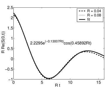
Figure 5: Real part of the time-dependent structure factor $S(0,t)$ obtained from our numerical simulation. The results above are for $U/R=8.33$. Two different values of $R$ are shown, and the axes have been scaled to demonstrate the scaling collapse as required by Eq. (22). The fit with the functional form in Eq. (26) is also shown.

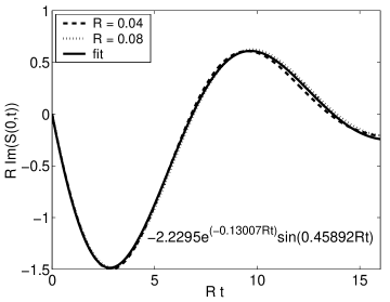
Figure 6: As in Fig. 5, but for the imaginary part of the correlation function.

We have fit each observed time evolution to the functional form

$$\Phi_{t}\approx Ze^{-R(i\omega_{0}\overline{t}+\gamma|\overline{t}|)},$$ (26)

where $Z$, $\omega_{0}$, $\gamma$ are numbers determined from the fit. A sample fit is shown in Figs. 5 and 6. As is clear from the figures, this form provides an excellent fit over a substantial time window. Taking the Fourier transform of this result, and using Eq. (23), we obtain a result for $S_{\psi}(\omega)$ in the form in Eq. (9), with the same parameters $Z$, $\omega_{0}$, $\gamma$.

The results for $Z$ appeared earlier in Fig. 4, and our results $\omega_{0}$ and $\gamma$ as a function of $U/R$ appears in Figs. 7 and 8.

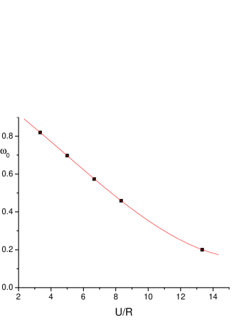
Figure 7: The universal dependence of the dimensionless frequency $\omega_{0}$ on $U/R$. The points are the results of the numerical simulation, while the line is a best fit polynomial used for interpolation.

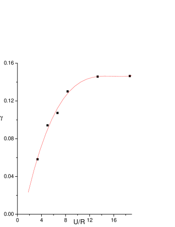
Figure 8: As in Fig 7, but for the dimensionless damping $\gamma$. The full line at small $U/R$ is the result of the perturbation theory obtained in Eq. (30).

We can now combine the results in these figures with those in Fig 3, and obtain predictions for the $T$ dependence of the resonant frequeny and damping in the dynamic structure factor in Eq. (9) at the quantum-critical point. These results appear in Fig 9 and 10.

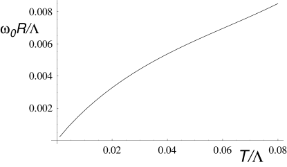
Figure 9: The universal dependence of the oscillation frequency $\omega_{0}R$ on $T$ at the quantum-critical point $\mu=0$, obtained from Figs. 3 and 7.

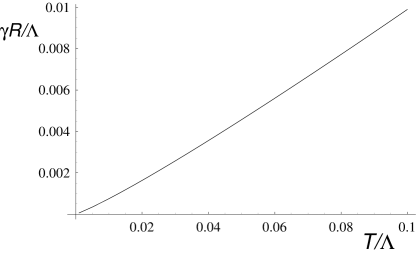
Figure 10: The universal dependence of the damping rate $\gamma R$ on $T$ at the quantum-critical point $\mu=0$, obtained from Figs. 3 and 8.

III Conclusions

This paper has argued that the quantum-critical dynamics of the two-dimensional Bose gas (and of other quantum critical points in two spatial dimensions) represents a strong-coupling problem. Nevertheless, an effective classical description was obtained to leading logarithmic order, allowing tractable numerical simulation. The primary results of this simulation at the quantum critical point appear in Figs. 9 and 10, which specify the parameters appearing in Eq. (9).

In comparing our results to experiments, we have to set the value of the unknown high energy cutoff $\Lambda$. For the range of parameters shown in Figs. 9 and 10, we find a roughly linear dependence of $\omega_{0}R$ and $\gamma R$ on $T$, with $\omega_{0}R\approx 0.11(k_{B}T)$ and $\gamma R\approx 0.10(k_{B}T)$. The experiments stone ; stone2 ; hong on the quantum-critical point of PHCC, also observe a roughly linear dependence of peak frequency and width on temperature, but with different co-efficients; the peak frequency $\approx 0.62k_{B}T$, while the width is $\approx 0.23k_{B}T$. Choosing a different range of $\Lambda$ for the theory, e.g. assuming the experiments are in the range $T/\Lambda<0.01$, will change the theoretical predictions for $\omega_{0}R$ and $\gamma R$, but does not improve the agreement with experiments.

For the peak frequency, the work of Ref. hong, suggests an origin for the above discrepancy. A similar theory was used in that paper to obtain the predictions of the peak frequency, but keeping the full lattice dispersion for the spin excitations, and the quantum Bose function values for the occupation numbers: good agreement was found between such a theory and the experimental observations. The continuum and classical limits taken in the present paper were avoided.

For the width of the spin excitation, we expect that the damping is more strongly dominated by the low energy and low momentum excitations, and so the present continuum, classical theory should yield a more accurate description of the experiments. This is indeed the case, relative to the poor accuracy of the peak frequency in the continuum theory. Nevertheless, a discrepancy of a factor of $\approx 2$ remains between our present quantum critical theory and the experimental observations. It is possible that taking the classical theory also on the lattice will improve agreement with experiments. However, there are also corrections to the present continuum theory which could improve the situation: in particular, at higher order in $V_{R}$, there appear renormalization of the time-derivative term in Eq. (1). This renormalization would change the time-scale in the classical equations of motion, and so change the overall frequency scale of the results in Figs. 9 and 10.

Appendix A Pertubation theory

Here we present the results of a direct perturbative computation of $\chi_{\psi}$. To order $U^{2}$, perturbation theory yieldsss1

$$\chi_{\psi}(\omega)=\frac{1}{-\hbar\omega+R+\Sigma(\omega)}$$ (27)

where

$$\Sigma(i\omega)=-2U^{2}\sum_{\epsilon_{1},\epsilon_{2}}\int\frac{d^{2}k_{1}}{4\pi^{2}}\frac{d^{2}k_{2}}{4\pi^{2}}\frac{1}{(-i\epsilon_{1}+k_{1}^{2}+R)(-i\epsilon_{2}+k_{2}^{2}+R)(-i(\epsilon_{1}+\epsilon_{2})+i\omega+(k_{1}+k_{2})^{2}+R)}.$$

The frequency summation is done most easily by partial fractions and yields

$$\Sigma(i\omega) = -2\left(\frac{U}{k_{B}T}\right)^{2}\int\frac{d^{2}k_{1}}{4\pi^{2}}\frac{d^{2}k_{2}}{4\pi^{2}}\frac{\left[n(k_{1}^{2}+R)-n((k_{1}+k_{2})^{2}+R)\right]\left[n(k_{2}^{2}+R)-n((k_{1}+k_{2})^{2}-k_{1}^{2})\right]}{i\omega+(k_{1}+k_{2})^{2}-k_{1}^{2}-k_{2}^{2}-R}.$$

Now we analytically continue to real frequencies, and take the imaginary part at $\omega=R/\hbar$, which is the leading order position of the pole in Eq. (27). This yields

$$\mbox{Im}\Sigma(R/\hbar) = 2\pi\left(\frac{U}{k_{B}T}\right)^{2}\int\frac{d^{2}k_{1}}{4\pi^{2}}\frac{d^{2}k_{2}}{4\pi^{2}}\left[n(k_{1}^{2}+R)-n((k_{1}+k_{2})^{2}+R)\right]$$ (28)

$$~{}~{}~{}~{}~{}~{}~{}~{}\times\left[n(k_{2}^{2}+R)-n((k_{1}+k_{2})^{2}-k_{1}^{2})\right]\delta((k_{1}+k_{2})^{2}-k_{1}^{2}-k_{2}^{2})$$

$$= -2\pi\left(\frac{U}{k_{B}T}\right)^{2}\int\frac{d^{2}k_{1}}{4\pi^{2}}\frac{d^{2}k_{2}}{4\pi^{2}}\left[n(k_{1}^{2}+R)-n(k_{1}^{2}+k_{2}^{2}+R)\right]\left[n(k_{2}^{2})-n(k_{2}^{2}+R)\right]$$

$$~{}~{}~{}~{}~{}~{}~{}~{}~{}~{}~{}~{}~{}~{}~{}~{}~{}~{}~{}~{}~{}~{}~{}~{}~{}~{}~{}~{}~{}~{}~{}~{}~{}~{}\times\delta((k_{1}+k_{2})^{2}-k_{1}^{2}-k_{2}^{2}).$$

Now we can do the angular integration because the angle appears only in the argument of the delta function, and obtain

$$\mbox{Im}\Sigma(R/\hbar) = -\left(\frac{U}{2\pi k_{B}T}\right)^{2}\int_{0}^{\infty}\!dk_{1}\int_{0}^{\infty}\!dk_{2}\frac{(e^{R/(k_{B}T)}-1)}{(e^{(k_{1}^{2}+R)/(k_{B}T)}-1)(e^{(k_{2}^{2}+R)/(k_{B}T)}-1)(1-e^{-(k_{1}^{2}+k_{2}^{2}+R)/(k_{B}T)})}.$$ (29)

This result is a function of $R/(k_{B}T)$ which has to be evaluated numerically. However, it is instructive to examine its value in the classical limit, upon applying the approximation in Eq. (20), when we obtain

$$\mbox{Im}\Sigma(R/\hbar) = -\frac{U^{2}R}{4\pi^{2}}\int_{0}^{\infty}\!dk_{1}\int_{0}^{\infty}\!dk_{2}\frac{1}{(k_{1}^{2}+R)(k_{2}^{2}+R)(k_{1}^{2}+k_{2}^{2}+R)}$$ (30)

$$= -R\left(\frac{U}{R}\right)^{2}\frac{(4-\pi)}{16\pi}.$$

Notice that explicit factors of $k_{B}T$ have dropped out, and consequently Eqs. (27) and (30) are consistent with the scaling form Eq. (9). It is also interesting to compare the value of the classical limit in Eq. (30) with that obtained from the full quantum expression in Eq. (29). For $R=k_{B}T/2$ (which are roughly the quasiparticle energy values obtained in the experiments on PHCC hong ), Eq. (29) evaluates to a value which is 16% smaller than Eq. (30). This gives us an estimate of the error made by representing the quantum-critical theory by classical equations of motion.

References

- (1) A. Oosawa, T. Takamasu, K. Tatani, H. Abe, N. Tsujii, O. Suzuki, H. Tanaka, G. Kido, and K. Kindo, Phys. Rev. B 66, 104405 (2002).
- (2) S. E. Sebastian, P. A. Sharma, M. Jaime, N. Harrison, V. Correa, L. Balicas, N. Kawashima, C. D. Batista, and I. R. Fisher, cond-mat/0502374.
- (3) V. S. Zapf, D. Zocco, M. Jaime, N. Harrison, A. Lacerda, C. D. Batista, and A. Paduan-Filho, cond-mat/05005562.
- (4) M. B. Stone, I. Zaliznyak, D. H Reich, and C. Broholm, Phys. Rev. B 64, 144405 (2001).
- (5) M. B. Stone, C. Broholm, D. H. Reich, P. Vorderwisch, and N. Harrison, cond-mat/0503450.
- (6) T. Hong, E. R. Dunkel, S. Sachdev, M. Kenzelmann, M. Stone, M. Bouloubasis, C. Broholm, and D. Reich, to appear.
- (7) S. Sachdev, T. Senthil, and R. Shankar, Phys. Rev. B 50, 258 (1994).
- (8) V. N. Popov, Functional Integrals in Quantum Field Theory and Statistical Physics (D. Reidel, Boston, 1983).
- (9) D. S. Fisher and P. C. Hohenberg, Phys. Rev. B 37, 4936 (1988).
- (10) D. Podolsky, A. Vishwanath, J. Moore, and S. Sachdev, to appear.
- (11) J. A. Hertz, Phys. Rev. B 14, 1165 (1976).
- (12) T. Moriya and J. Kawabata, J. Phys. Soc. Japan 34, 639 (1973); 35 ,669 (1973).
- (13) A. J. Millis, Phys. Rev. B 48, 7183 (1993).
- (14) S. Sachdev, Phys. Rev. B 59, 14054 (1999).
- (15) N. Prokof’ev, O. Ruebenacker, and B. Svistunov, Phys. Rev. Lett. 87, 270402 (2001).
- (16) N. Prokof’ev and B. Svistunov, Phys. Rev. A 66, 043608 (2002).
- (17) S. Sachdev and E. Demler, Physical Review B 69, 144504 (2004).
- (18) D. Dalidovich and P. Phillips, Phys. Rev. B 63, 224503 (2001); 66, 073308 (2002).
- (19) S. Sachdev, Quantum Phase Transitions (Cambridge University Press, Cambridge, 1999).