Spin gaps and magnetic structure of Na_xCoO₂

Abstract

We present two experiments that provide information on spin anisotropy and the magnetic structure of Na_xCoO₂. First, we report low-energy neutron inelastic scattering measurements of the zone-center magnetic excitations in the magnetically ordered phase of Na_0.75CoO₂. The energy spectra suggest the existence of two gaps, and are very well fitted by a spin-wave model with both in-plane and out-of-plane anisotropy terms. The gap energies decrease with increasing temperature and both gaps are found to have closed when the temperature exceeds the magnetic ordering temperature $T_{m}\approx 22$ K. Secondly, we present neutron diffraction studies of Na_0.85CoO₂ with a magnetic field applied approximately parallel to the $c$ axis. For fields in excess of $\sim 8$ T a magnetic Bragg peak was observed at the $(0,0,3)$ position in reciprocal space. We interpret this as a spin-flop transition of the A-type antiferromagnetic structure, and we show that the spin-flop field is consistent with the size of the anisotropy gap.

I Introduction

Since the discovery of superconductivity in water-intercalated Na_xCoO₂ takada-2003 much of the discussion has focussed on the mechanism of superconductivity. There is strong support from experiment experimental-evidence and theory mazin-2005 ; theoretical-evidence for an unconventional pairing state, the origin of which derives from the triangular lattice of the Co ions and the existence of strong spin and charge fluctuations. However, details of the pairing state are far from resolved. mazin-2005 The phase diagram of Na_xCoO₂ shows two magnetically ordered phases, one at $x\approx 0.5$ and the other in the range $x\approx 0.7-0.95$. The presence of these suggests that magnetic correlations may play an important role in the formation of superconductivity in hydrated Na_xCoO₂, as is believed to be the case for the superconducting cuprates. This possibility provides a strong incentive for characterizing the magnetic order and excitations of Na_xCoO₂.

Figure 1: (color online) (a) Crystal structure of Na_xCoO₂. (b) The A-type antiferromagnetic structure on which the spin-wave model is based, showing the two exchange constants $J_{ab}$ and $J_{c}$. (c) The $a$–$b$ planes, showing the orientation of the oxygen tetrahedron around a central Co ion.

This paper is concerned with the weakly magnetic phase found for $x\approx 0.7-0.95$ at temperatures below $T_{m}\approx 22$ K.Motohashi-2003 ; Sugiyama-2004 Recent neutron scattering studies of Na_0.75CoO₂ boothroyd-may04 ; helme-2005 and Na_0.82CoO₂ bayrakci-2005 have established that the magnetic order and dynamics are consistent with an A-type antiferromagnetic structure, shown in Fig. 1, and that the magnetic interactions are three-dimensional despite the two-dimensional character of the crystal lattice and electronic structure. Reasons for the relatively strong $c$-axis magnetic coupling have been discussed recently by Johannes et al.Johannes-2005 Surprisingly, although the magnetic correlations are rather strong the ordered moment is only 0.1–0.2 $\mu_{\rm B}$.Sugiyama-2003 ; bayrakci-2005

The first aim of this work was to extend the measurements of the spin-wave dispersion in Na_0.75CoO₂ down to lower energies where we might gain important information on the magnetic ground state, such as whether itinerant effects are important. Our previous measurements,helme-2005 as well as those by Bayrakci et al. on Na_0.82CoO₂,bayrakci-2005 found evidence of a small excitation gap at the antiferromagnetic zone center. Here we present a detailed study of the spectral lineshape in this low-energy region which not only confirms that the magnetic excitation spectrum is gapped, but also provides evidence for the existence of two gaps. Both these gaps are found to close at the bulk magnetic transition temperature $T_{m}\approx$22 K.

The second part of the paper presents a novel way to investigate the magnetic structure of Na_xCoO₂ ($x\approx 0.7-0.95$) and also to gain information about spin anisotropy. In the accepted A-type antiferromagnetic structure (Fig. 1b) the moments are ferromagnetically aligned within the layers and stacked antiferromagnetically along the $c$ axis.helme-2005 ; bayrakci-2005 The ordering wavevector for this structure is $(0,0,1)$. Strong spin-wave scattering is observed emerging from $(0,0,l)$ positions with odd $l$, which are zone centers for the A-type antiferromagnetic order, but no magnetic Bragg peaks have been observed at these positions using neutrons. On this basis it was deduced that the ordered moments point along the $c$ direction since neutrons scatter from the component of the moments perpendicular to the scattering vector. This moment direction is consistent with what has been inferred from the uniform susceptibility and from $\mu$SR data.moment-reference Moreover, Bayrakci et al. did succeed recently in observing magnetic Bragg reflections at a few $(h,k,l)$ positions with $h$, $k\neq 0$ and odd $l$ using polarized neutrons.bayrakci-2005 Again, these are consistent with the accepted magnetic structure. Polarized neutrons were required because the ordered moment is small and strong non-magnetic scattering is observed at all positions where magnetic Bragg peaks are expected. Up to now no magnetic Bragg peaks have been observed with unpolarized neutrons.

The experiment we describe here was originally designed to confirm the proposed magnetic structure by a method that employs unpolarized neutrons but avoids the problem of having to separate the weak magnetic scattering from the strong non-magnetic background signal. Our approach was motivated by measurements of the magnetization of Na_0.85CoO₂ in applied fields up to 14 T by Luo et al.. luo-2004 The magnetization data with $H\parallel c$ show a clear anomaly at 8 T at low temperatures, with no such transition seen for $H\perp c$. The authors interpreted this as a spin-flop transition in which the ordered moments rotate by $\sim$90 degrees while preserving the A-type antiferromagnetic arrangement. After the transition the spins lie approximately in the hexagonal plane, but the magnetic structure has a small ferromagnetic component along the $c$ axis. Assuming this explanation to be correct we induced the spin-flop transition in a neutron diffraction experiment and searched for magnetic Bragg peaks along ${\bf Q}=(0,0,l)$, since now the ordered moment should be perpendicular to the scattering wavevector and should scatter neutrons. Our experimental results are in excellent accord with the predicted behavior. Encouraged by this we go on to show that the size of the spin gap in the magnetic excitation spectrum is in agreement with the observed spin-flop field. This quantitative analysis provides the link between the static and dynamic magnetic properties explored in this paper.

The remainder of the paper is organized as follows. Inelastic neutron measurements probing the low-energy region of the spin-wave dispersion are presented in the next section, along with the analysis of these results. Diffraction measurements made with an external magnetic field applied parallel to the $c$ axis are presented and analyzed in Sec. III. Section IV contains a discussion of the results, and the conclusions are presented in Sec. V.

II Inelastic Measurements

II.1 Experimental Details

Inelastic neutron measurements were performed on the cold-neutron triple-axis spectrometer IN14 at the Institut Laue-Langevin. This instrument was chosen to allow investigation of the excitations in Na_0.75CoO₂ at lower energies than previously studied.helme-2005 We employed a pyrolytic graphite (PG) $(002)$ monochromator and a PG $(002)$ analyzer, which were curved vertically and horizontally respectively to maximize the count rate. The majority of measurements were made with a fixed final energy of $E_{\rm f}$ = 4 meV. A Beryllium filter was placed in the scattered beam to suppress higher-order harmonics.

The inelastic neutron measurements were performed on the same crystal of Na_0.75CoO₂ as used for our previous experiments which investigated the spin fluctuations in this compound at higher energies.helme-2005 The single crystal of mass $\sim 1.5$ g was mounted on a copper mount and aligned to allow measurements to be made within the $(100)$–$(001)$ scattering plane. Details of the growth and mounting are given elsewhere. helme-2005 ; prabhaks-paper

Previous measurements revealed strong spin-wave scattering around (0,0,1) and (0,0,3), consistent with the proposed A-type antiferromagnetic structure, and the inelastic data presented here concentrates on spin waves dispersing from the magnetic zone center at (0,0,1), where the inelastic scattering is most intense.

II.2 Results

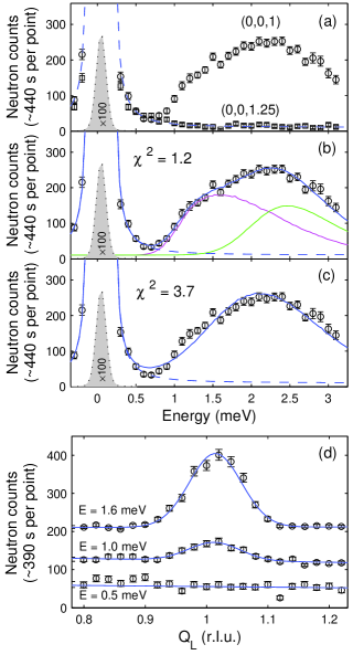
Figure 2: (color online) Neutron inelastic scattering from Na_0.75CoO₂ measured at $T=1.5$ K. (a) Energy scan at constant ${\bf Q}=(0,0,1)$, compared with the same scan at a background position ${\bf Q}=(0,0,1.25)$. (b, c): The data at ${\bf Q}=(0,0,1)$, fitted (solid line) with (b) a two-mode dispersion (Eqn.2), and (c) one mode only (Eqn.2 but with $E\equiv 0$). The two peaks under the data in (b) show the contribution of each mode to the total intensity, while in (a-c) the dashed curve represents the contribution of the incoherent peak and background. The shaded peaks show the incoherent peak contribution scaled down by a factor of 100, as an indication of the instrumental resolution. (d) ${\bf Q}_{l}$ scans with constant energy transfers of 0.5 meV, 1.0 meV and 1.6 meV. Data at 1.0 meV and 1.6 meV have been shifted up by 100 and 200 counts respectively for clarity.

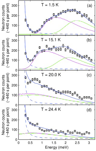
Figure 3: (color online) (a)-(d) Energy scans at ${\bf Q}=(0,0,1)$ at temperatures between $T=1.5$ K and 24.4 K. Solid curves represent the best fit of Eqn.2 plus an incoherent peak to the data. The dashed line shows the contribution of the incoherent peak and background, while the pink and green curves represent the intensities of each mode.

Figures 2 and 3 present examples of inelastic neutron scattering data collected on IN14. Each scan was performed by measuring the intensity of scattered neutrons as a function of energy transfer up to $\sim 3$ meV at the wavevector ${\bf Q}=(0,0,1)$. Scans were made at ten temperatures between 1.5 K and 24.4 K.

Figures 2a–c show the measurements made at low temperature ($T=1.5$ K). The spectrum consists of an intense peak due to incoherent nuclear elastic scattering centered on $E=0$ meV, and a broad signal centered around 2 meV which is attributed to magnetic scattering as the scan cuts through the spin-wave dispersion. There is clearly a gap where the intensity falls to background below $\sim 1$ meV, revealing that the magnetic excitations in Na_0.75CoO₂ are separated from the ordered ground state by a clean gap. To determine the non-magnetic scattering an energy scan was also made at ${\bf Q}=(0,0,1.25)$. The scan, which is plotted in Fig. 2a, contains the nuclear incoherent peak together with a small constant background signal. Figure 2d displays ${\bf Q}_{l}$ scans performed at three constant energy transfers of $E_{T}=0.5$, 1.0 and 1.6 meV. The peak present at higher energies has clearly disappeared at 0.5 meV, confirming that the intensity of the spin-wave dispersion really does fall to background in the ‘gap’, and the remaining intensity at this point seen in Fig.s 2a–c is simply due to the tail of the incoherent peak.

Figure 3 shows the same scan made at three more of the temperatures we measured, below and above the magnetic transition temperature $T_{m}\approx 22$ K. It appears that the magnetic scattering intensity moves lower in energy as the temperature increases. Somewhere around 20 K the gap seems to disappear, moving into the incoherent peak.

II.3 Analysis

To determine whether the gap is in fact decreasing with temperature, or whether what we see is simply the mode broadening and decreasing in intensity, it is necessary to compare the experimental results with a model of the excitations. The scan observed at 1.5 K (Fig.2a) is suggestive of a two-peak lineshape. In order to extend the spin-wave model introduced in our previous work helme-2005 to allow two non-degenerate gapped modes at ${\bf Q}=(0,0,1)$ we include two anisotropy terms. The Hamiltonian of this refined model is then:

$$\mathcal{H} = J_{ab}\sum_{\langle i,i^{\prime}\rangle}{\bf S}_{i}\cdot{\bf S}_{i^{\prime}}+J_{c}\sum_{\langle i,j\rangle}{\bf S}_{i}\cdot{\bf S}_{j}$$ (1)

$$-D\sum_{i}(S_{i}^{z})^{2}-E\sum_{i}[(S_{i}^{x})^{2}-(S_{i}^{y})^{2}]\;\;,$$

where $J_{ab}$ and $J_{c}$ are intra- and inter-layer exchange parameters, respectively, as in our previous work. helme-2005 The anisotropy constant $D$ quantifies the tendency of the spins to lie along the $c$ axis, while the term $E\sum_{i}[(S_{i}^{x})^{2}-(S_{i}^{y})^{2}]$, which has two-fold symmetry in the plane, is the simplest way to introduce in-plane anisotropy. We define $x$ parallel to $a$, $z$ parallel to $c$ and $y$ perpendicular to $x$ and $z$ so as to make a right-handed set. From the hexagonal arrangement of the Co ions within the $a$–$b$ layers of this compound one might propose a term with hexagonal symmetry for the in-plane anisotropy. However, with the quantization direction parallel to the $c$ axis a term with hexagonal symmetry does not lift the two-fold degeneracy of the spin-wave dispersion, so for the purposes of this analysis we use the Hamiltonian above (Eqn. 1).

The spin-wave dispersion resulting from this Hamiltonian can be calculated using standard methods, giving two modes:

$$\hbar\omega^{\pm}_{\mathbf{Q}}=2S\sqrt{(A_{\mathbf{Q}}+D)^{2}-(C_{\mathbf{Q}}\pm E)^{2}}\;\;,$$ (2)

where $\hbar\omega$ is the energy transfer, $S$ is the spin (here assumed to be $S$ = 1/2), ${\mathbf{Q}}=(h,k,l)$ is the wavevector, and $A_{\mathbf{Q}}$ and $C_{\mathbf{Q}}$ are defined in terms of the exchange couplings as

$$A_{\mathbf{Q}} = J_{ab}\{\cos(2\pi h)+\cos(2\pi k)+\cos[2\pi(h+k)]-3\}$$

$$+J_{c}$$

$$C_{\mathbf{Q}} = J_{c}\cos(\pi l).\;\;$$ (3)

The magnitude of the gaps at the magnetic zone center are then related to the exchange and anisotropy parameters as follows:

$$\hbar\omega_{gap}^{\pm}=2S\sqrt{(J_{c}+D)^{2}-(J_{c}\pm E)^{2}}\;.$$ (4)

Note that if $E=0$ only one gap results.

For the case when ${\mathbf{Q}}$ lies parallel to the ordered moment direction, such as at ${\mathbf{Q}}=(0,0,1)$ here, the inelastic neutron intensity is proportional to $S^{xx}(\mathbf{Q},\omega)+S^{yy}(\mathbf{Q},\omega)$, squires where

$$S^{xx}(\mathbf{Q},\omega) = 2S^{2}\frac{\{(A_{\mathbf{Q}}+D)-(C_{\mathbf{Q}}-E)\}}{\hbar\omega^{-}_{\mathbf{Q}}}$$ (5)

$$\;\times G^{-}(\omega-\omega^{-}_{\mathbf{Q}})f^{2}(\mathbf{Q})[n(\omega)+1]$$

$$S^{yy}(\mathbf{Q},\omega) = 2S^{2}\frac{\{(A_{\mathbf{Q}}+D)-(C_{\mathbf{Q}}+E)\}}{\hbar\omega^{+}_{\mathbf{Q}}}$$ (6)

$$\;\times G^{+}(\omega-\omega^{+}_{\mathbf{Q}})f^{2}(\mathbf{Q})[n(\omega)+1]\;\;,$$

where $[n(\omega)+1]$ is the Bose factor, and $f(\mathbf{Q})$ is the form factor (which is a constant here since all our energy scans were made at one fixed value of $\mathbf{Q}$). $G(\omega-\omega^{\pm}_{\mathbf{Q}})$ are normalized Gaussian functions which replace the usual Delta functions to allow inclusion of intrinsic broadening of the two modes.

The triple-axis spectrometer has a three-dimensional ellipsoid-shaped resolution, and therefore does not probe the dispersion relation at an infinitely sharp point in reciprocal space. In order to fit the spin-wave model to the experimental data it was therefore necessary to convolute the calculated spectrum (Eqns. 5 and 6) with the IN14 spectrometer resolution. This was achieved using RESCAL, a set of programs integrated into Matlab which calculates the resolution function of the neutron triple-axis spectrometer.rescal It allows simulation of scans using a 4D Monte-Carlo convolution of the resolution function with the specified spectrum, and the simulation can then be fitted to the data in order to extract the parameters.

In this way the anisotropy parameters were extracted, while fixing the exchange parameters $J_{ab}$ and $J_{c}$ to their previous values of $-6$ meV and 12.2 meV respectively. helme-2005 The relative amplitudes of the two modes were fixed by the spin-wave model, with an overall amplitude fitted, the values for the intrinsic widths of the dispersion modes were fitted independently. The incoherent peak and background were included as a fixed Voigtian peak plus a constant.

At $T=1.5$ K the values for $D$ and $E$ were found to be $0.096\pm 0.005$ and $0.059\pm 0.005$ meV, corresponding to two modes with gaps of $0.95\pm 0.13$ and $1.95\pm 0.06$ meV. To achieve a good fit the intrinsic widths of the two modes were found to be different, 0.37 and 0.74 meV for the lower and higher modes. The fitted curve is displayed on Fig.2a, with the two lower curves representing the contribution of each of the gapped modes. The dashed line shows the contribution of the incoherent peak, which is also plotted scaled down by a factor of 100 (shaded peak) as an indication of the instrumental resolution.

The model appears to fit the data well. For comparison Fig. 2b shows the same data fitted with a ‘one-mode’ dispersion, by fixing the value of $E$ to zero. It is clear that the model with two modes fits the data better than that with one, yielding a value of $\chi^{2}$=1.2 compared to $\chi^{2}$=3.7 with $E=0$. In Fig. 4 we plot the two dispersion modes parallel to ${\bf Q}_{l}$ (calculated from Eqn. 2 using the fitted parameters for $D$ and $E$), together with the data previously measured around ${\bf Q}=(0,0,3)$. The fitted modes are also in good agreement with the experimental data in the ${\bf Q}_{l}$ direction.

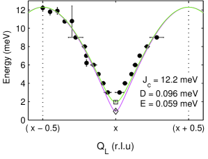
Figure 4: (color online) Filled circles: Magnon dispersion parallel to $(0,0,l)$ centered on $(0,0,x)$=$(0,0,3)$, measured previously.helme-2005 Open square/diamond: Fits to 1.5 K energy scan at $(0,0,x)$=$(0,0,1)$ shown in Fig.2. Solid curves are modes calculated from the spin-wave dispersion Eqn.2 with the constants given, while dotted lines represent the zone boundaries.

The fitting procedure was repeated for data at all temperatures, restricted only by fixing the intrinsic widths of the two modes to the values at $1.5$ K. Figures 3a–d are overplotted with fits to each data set, with the contributions from each mode as solid lines underneath, and the contribution from the incoherent peak denoted by the dashed line. The fitted lines provide a reasonable description of the data, reproducing the shift of the intensity towards zero energy with increasing temperature, although clearly the lineshapes fit less well as the temperature increases. The gap energies extracted from these fits are plotted as a function of temperature in Fig. 5.

Both gaps are seen to decrease with temperature, falling to near zero at $\approx 20$ K. Above $20$ K the fitted gaps are relatively constant and close to zero.

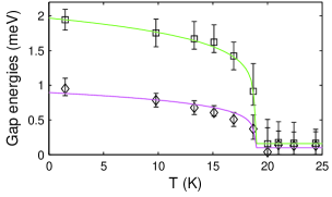
Figure 5: (color online) The magnitudes of the two gaps as a function of temperature. Data points calculated from Eqn.4 using the values of $J_{c}$, $D$ and $E$ derived from fits such as those in Fig.3. Solid curves are guides for the eye. Error bars were estimated by varying the two gap energies separately until the fit was no longer acceptable.

III Diffraction Measurements

III.1 Experimental Details

Neutron diffraction measurements were performed on the hot-neutron diffractometer D3 at the Institut Laue-Langevin. The instrument was used in unpolarized-neutron mode with a neutron wavelength of 0.84 Å. The single crystal of Na_0.85CoO₂ used for these measurements was cleaved from a rod grown in Oxford by the floating-zone method.prabhaks-paper The crystal had a mass of 0.3 g and a mosaic spread of $\sim 2$ degrees.

Magnetization measurements made using a SQUID magnetometer in Oxford confirmed the existence of the metamagnetic transition at $\sim 9$ T reported by Luo et al. at this composition. luo-2004

The crystal was pre-aligned on the neutron Laue diffractometer Orient Express at the ILL and mounted on an aluminium pin using ceramic glue. The ideal setup for this experiment would be to align the $c$ axis vertically, applying a vertical field, with the incident and scattered beams inclined at the Bragg angle to the horizontal in order to access the $(0,0,3)$ reflection. An alternative setup, with a fixed horizontal incident beam, would require the cryomagnet holding the sample to be tilted by the Bragg angle ($\theta_{B}$), with the detector lifted out of the plane (by $2\theta_{B}$), allowing access to the $(0,0,3)$ reflection while still applying the field directly along the $c$ axis.

However, on D3 we were restricted to using a horizontal incident beam (ruling out the first setup), and also unable to tilt the cryomagnet (ruling out the second). In order to access the $(0,0,3)$ reflection we tilted the crystal $c$ axis $7$ degrees away from vertical, corresponding to the $(0,0,3)$ Bragg angle for 0.84 Å neutrons, and lifted the detector out of the horizontal plane by 14 deg. The 10 Tesla vertical-field cryomagnet in which the crystal was mounted then allowed application of a field almost parallel to the $c$ axis (though actually $7$ degrees away from it). The field-induced (0,0,1) magnetic Bragg peak is expected to be larger than that at (0,0,3) due to the magnetic form factor, but with 0.84 Å neutrons the scattering angle for (0,0,1) is too small to access with our setup.

III.2 Results

Figure 6: Diffraction studies of Na_0.85CoO₂. (a) Field scans at ${\bf Q}=(0,0,3)$ at constant temperatures of $T=1.8$, 10 and 30 K. Data at $T=10$ K and 30 K are shifted up by 500 and 1000 counts respectively. (b) Temperature scans at ${\bf Q}=(0,0,3)$, with zero applied field (open circles), and with $H=$9.6 T applied at 7 degrees to the $c$-axis (filled circles).

Figure 6 shows the main results of the diffraction studies of Na_0.85CoO₂. All the measurements were made at ${\bf Q}=(0,0,3)$, scanning either field or temperature with the other external variable fixed. For ideal Na_xCoO₂ no structural Bragg peak is allowed at this position and no magnetic Bragg peak is allowed if the moments point along the $c$ axis.

Figure 6a shows three field scans at ${\bf Q}=(0,0,3)$, performed at constant temperatures of $T=1.8$, 10 and 30 K. The data at 10 K and 1.8 K have been shifted up by 500 and 1000 counts respectively for clarity.

At $T=1.8$ K there is a large increase in the intensity of scattering at $(0,0,3)$ between $\sim$6 T and 9 T as the field increases, with the intensity appearing to flatten off between 9 and 10 T. At $T=10$ K the increase in intensity has shifted up in field to start at $\sim$8 T, and at $T=30$ K the intensity remains constant with field. The increase in intensity with field at 1.8 K is consistent with the expected spin-flop transition because once the spins have rotated away from the $c$ direction magnetic Bragg scattering is allowed at $(0,0,3)$ provided that the ordering wavevector remains $(0,0,1)$.

With increasing temperature two effects are at work: (1) the field at which the spin-flop transition occurs shifts up slowly with $T$,luo-2004 and (2) the ordered magnetic moment $\mu$ decreases with $T$. Both effects would result in the reduction of intensity with increasing temperature. However, the effect of (1) is too small to explain the disappearance of the signal by 30 K (see Luo et al. luo-2004 ), so we deduce that the signal disappears due to the reduction of the magnetic moment to zero above the magnetic ordering temperature $T_{m}$.

In Fig. 6b we plot the temperature dependence of the scattering at ${\bf Q}=(0,0,3)$, in both zero applied field and 9.6 T. We confirm that the signal induced by application of the magnetic field decreases to zero as the temperature is raised to $\sim 20$ K.

III.3 Analysis

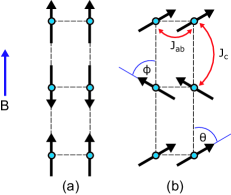
Figure 7: (color online) (a) The ordered A-type antiferromagnetic structure in the $a$–$c$ plane, with an external magnetic field ${\bf B}$ applied parallel to the magnetic moments. (b) Above a critical field $B_{sf}$ the system undergoes a spin-flop transition, to a phase with spins at an angle $\theta=\phi$ to the $c$-axis.

Figure 7 shows the magnetic structure of the low-field A-type antiferromagnetic (AF) phase (a), along with that of the spin-flop (SF) phase (b). As discussed above, the large increase in Bragg intensity at ${\bf Q}=(0,0,3)$ that occurs between $\sim 6$ T and 9 T (Fig. 6(a)) appears to support the idea that a phase transition from an AF to a SF phase occurs at this field. To connect the spin-flop transition with the anisotropy gap described in Section II we extend the spin-wave model to include an external magnetic field applied along the $c$ axis. We begin by calculating the effect of the field on the spin-wave modes of the AF phase. This enables us to calculate the critical field at which a phase transition would be expected to occur. A term is added to the original Hamiltonian to represent a vertical applied magnetic field, giving a new Hamiltonian:

$$\mathcal{H}^{\prime}=\mathcal{H}+g\mu_{B}B\sum_{i}S_{i}^{z}\;,$$ (7)

where $\mathcal{H}$ is the original Hamiltonian (Eqn.1), $B$ is the magnitude of the applied magnetic field, and we assume $g=2$.

The spin-wave dispersion was derived from $\mathcal{H}^{\prime}$ as before. The field further splits the two modes, i.e. the lower mode moves lower in energy, and the higher mode moves higher in energy, as the field is increased. The magnitude of the gaps at the magnetic zone center as a function of field, $B$, are then given by

$$\hbar\omega_{gap}^{\pm}(B) = 2S\Big{[}\beta^{2}+(2J_{c}D+D^{2}-E^{2})$$ (8)

$$\pm 2\sqrt{\beta^{2}D(2J_{c}+D)+J_{c}^{2}E^{2}}\Big{]}^{\frac{1}{2}}\;,$$

where $\beta=g\mu_{B}B/2S$.

As the field is increased to a critical field, $B_{c1}$, a local instability occurs when the energy of the lower mode falls to zero and then becomes imaginary, and the system can no longer remain in the low-field AF phase (Fig. 7a). The critical field is determined by setting $\hbar\omega_{gap}^{\pm}(B_{c1})=0$, resulting in the expression

$$B_{c1}=\frac{2S}{g\mu_{B}}\sqrt{(D-E)(2J_{c}+D-E)}\;.$$ (9)

$B_{c1}$ is the critical field at which we would expect the system to ‘flop’ out of the A-type antiferromagnetic phase (Fig. 7a) into the spin-flop phase (Fig. 7b) based on the closing of the gap with increasing field.

A similar calculation can be performed by considering the spin-wave modes in the SF phase, shown in Fig.7(b), with $\theta=\phi$. In this phase there are two modes at high field, and as the field is decreased there exists a critical field $B_{c2}$ at which the lower mode vanishes and the SF phase is no longer stable. At this field, $B_{c2}$, the system returns to the AF phase. By calculating the spin-wave dispersion in the SF phase we find the angle at which the spins lie in the $a$–$c$ plane, as a function of field,

$$\theta=\arccos\left(\frac{\mu B}{2S^{2}(2J_{c}-D+E)}\right)\;,$$ (10)

and an expression for the critical field, $B_{c2}$:

$$B_{c2}=\frac{2S}{g\mu_{B}}\sqrt{\frac{(D-E)(2J_{c}-D-E)^{2}}{(2J_{c}+D-3E)}}\;.$$ (11)

In a spin-flop transition $B_{c1}\geq B_{c2}$, so hysterisis is possible. By evaluating Eqns.9 and 11, using the values for the exchange and anisotropy constants determined by fitting the inelastic data on Na_0.75CoO₂ at 1.5 K (Section II C), we find values of $B_{c1}=8.19\pm 0.2$ T and $B_{c1}=8.15\pm 0.2$ T. Therefore the hysterisis is expected to be too small to measure, and we take $B_{c}=8.2\pm 0.2$ T as the critical field. This value is in strong agreement with the experimental data shown in Fig. 6a. When the spins ‘flop’ into the SF phase we calculate $\theta=87.8\pm 0.5$ degrees (from Eqn. 10), so the spins lie almost aniferromagnetically perpendicular to the applied magnetic field. We note that a mean-field approximation to this calculation also gives values $B_{c}=8.2\pm 0.2$ T and $\theta\approx 88$ degrees, and that corrections to this calculation to account for the field offset of 7 degrees from vertical are small and within the given errors.

An estimate of the magnetic moment was derived from the diffraction data by comparing the integrated intensities of a set of nuclear reflections with the integrated intensity of the (0,0,3) magnetic Bragg peak, using the A-type antiferromagnetic model for the magnetic structure. From this we estimate a magnetic moment of 0.11$\pm$0.07$\mu_{\rm B}$, in agreement with values derived by other techniques. moment-reference For this calculation we used the free-ion form factor for Co⁴⁺, which may not be a good approximation given the metallic nature of Na_0.85CoO₂.

IV Discussion

We have seen that the spin-wave dispersion does contain a clear gap, and that at low temperature (1.5 K) it is well described by our simple Hamiltonian extended to include two anisotropy terms (Eqn. 1). While including a term to describe a uniaxial anisotropy ($D$) seems logical given that the spins do lie along the $c$ axis, the need to introduce also an in-plane anisotropy term, with parameter $E$ nearly two thirds as large as the uniaxial parameter $D$, was unexpected. Although the form of the in-plane anisotropy term may need more careful thought, we have shown that in-plane anisotropy clearly exists in the compound: the data cannot be described with the uniaxial anisotropy alone. The magnitudes of the anisotropies $D$ and $E$ (0.096 and 0.059 meV respectively at 1.5 K) are very small in comparison to the exchange parameters $J_{c}$ and $J_{ab}$ (12.2 and 6 meV). To refine the model further with a more realistic form for the spin anisotropy would require a more detailed consideration of the source of the anisotropy.

By fitting the same model to data measured at various temperatures up to 24.4 K we have shown that both gaps disappear quite suddenly at approximately 20 K. From the proximity of this temperature to the bulk magnetic transition at $T_{m}\approx 22$ K found in magnetization studies we infer that the spin waves have the same origin as the $T_{m}$ transition. This may seem obvious, but the strength of the spin-wave scattering in comparison to the small size of the ordered moment made it important to confirm that the observed spin excitations were really associated with the magnetic order.

We have successfully observed the magnetic Bragg peak at ${\bf Q}=(0,0,3)$ in Na_0.85CoO₂ with unpolarized neutrons by inducing a spin-flop transition in a vertical magnetic field. The transition occurred at a field of $B_{sf}\approx 8$ T, but was broad, with a width of approximately 3 T. It is possible that the broadening of the transition may be due to disorder in the structure, which would lead to a spread of values of the interlayer exchange constant $J_{c}$ and in turn lead to a range of values for $B_{sf}$.

We have presented a simple calculation of the spin-flop transition field that would be expected based on the anisotropy parameters derived from the measurement of the spin gap in Na_0.75CoO₂. The calculated value for this critical field of $8.2\pm 0.2$ T is in strong agreement with the observed value for Na_0.85CoO₂ of $B_{sf}\approx 8$ T. We take this as further evidence that the A-type antiferromagnetic structure with its associated gapped spin excitations is the same phase marked by the transition temperature $T_{m}\approx$22 K in magnetization data.

Although we have confirmed the magnetic structure and characterized the excitation gap, the nature of the magnetic ground state in Na_xCoO₂ is still in question. In an ionic picture there are $(1-x)$ Co⁴⁺ ions carrying spin $S=\frac{1}{2}$ in a background of $x$ Co³⁺ ions, which are usually assumed to be non-magnetic. However, it is uncertain whether these ions would be ordered or clustered or randomly distributed, helme-2005 and there is also evidence that Na_xCoO₂ is a good metal, which would suggest that an itinerant picture might be more appropriate.itinerant A weakly itinerant ground state with strong spin fluctuations would be consistent with both the small ordered moment ($\leq 0.2\mu_{B}$) and the fact that the energy scale of the magnetic excitations is much greater than the magnetic ordering temperature.

In this vein, the clean gap we have observed in the spin-wave dispersion points towards a system of local moments with a small symmetry-breaking anisotropy field, which is supported by our successful description of the data using a simple spin-wave model based on localized Co spins. However, the large intrinsic widths are not consistent with a model of purely localized Co ions, and can be taken as evidence of more metallic behavior. These features of the magnetism of Na_xCoO₂ need to be taken into consideration when assessing theories of the metallic state of this material.

V Conclusions

We have studied the low-energy region of the excitations in Na_0.75CoO₂ and revealed that the excitations are gapped. At low temperature the data were modelled best with a simple spin-wave model with two non-degenerate modes, providing evidence for both uniaxial and in-plane anisotropy in the compound. Gaps from both modes were found to close at the bulk magnetization temperature $T_{m}\approx 22$ K. We therefore conclude that the spin waves observed in Na_0.75CoO₂ are associated with the magnetic phase transition seen previously in magnetization data.

Furthermore, we have confirmed the A-type antiferromagnetic structure underlying these excitations by performing neutron diffraction measurements on Na_0.85CoO₂ in a large vertical applied magnetic field. A spin-flop transition occurs at $\approx 8$ T allowing measurement of the magnetic Bragg peak at ${\bf Q}=(0,0,3)$. The results support the assumption that the spins lie along the $c$ axis. We have calculated the field needed to overcome the anisotropy associated with the gap in the spin-wave dispersion and shown that it is in good agreement with the observed spin-flop transition field.

- (1) K. Takada et al., Nature (London) 422, 53 (2003).
- (2) M. Kato et al., cond-mat/0306036; Y. Kobayashi et al., J. Phys. Soc. Japn. 74, 1800 (2005); H. D. Yang et al., Phys. Rev. B 71, 020504(R) (2005); W. Higemoto et al., Phys. Rev. B 70, 134508 (2004); A. Kanigel et al., Phys. Rev. Lett. 92, 257007 (2004); M. Yokoi et al., J. Phys. Soc. Japn. 73, 1297 (2004); Y. J. Uemura et al., cond-mat/0403031; T. Fujimoto et al., Phys. Rev. Lett. 92, 047004 (2004); K. Ishida et al., J. Phys. Soc. Japn. 72, 3041 (2003); Y. Kobayashi et al., J. Phys. Soc. Japn. 72, 2453 (2003).
- (3) I. I. Mazin and M. D. Johannes, cond-mat/0506536.
- (4) Y. Yanase, M. Mochizuki, and M. Ogata, J. Phys. Soc. Japn. 74, 430 (2005); T. Watanabe et al., J. Phys. Soc. Japn. 73, 3404 (2004); D. Sa, M. Sardar, and G. Baskaran, Phys. Rev. B 70, 104505 (2004); M. D. Johannes et al., Phys. Rev. Lett. 93, 097005 (2004); K. Kuroki, Y. Tanaka, and R. Arita, Phys. Rev. Lett. 93, 077001 (2004); O. I. Motrunich and P. A. Lee, Phys. Rev. B 69, 214516 (2004).
- (5) T. Motohashi et al., Phys. Rev. B 67, 064406 (2003).
- (6) J. Sugiyama et al., Phys. Rev. B 69, 214423 (2004).
- (7) A. T. Boothroyd et al., Phys. Rev. Lett. 92, 197201 (2004).
- (8) L. M. Helme et al., Phys. Rev. Lett. 94, 157206 (2005).
- (9) S. P. Bayrakci et al., Phys. Rev. Lett. 94, 157205 (2005).
- (10) M.D. Johannes, I.I. Mazin, and D.J. Singh, Phys. Rev. B 71, 214410 (2005).
- (11) J. Sugiyama et al., Phys. Rev. B 67, 214420 (2003).
- (12) J. Sugiyama et al., Phys. Rev. B 67, 214420 (2003); S. P. Bayrakci et al., Phys. Rev. B 69, 100410(R) (2004).
- (13) J. L. Luo et al., Phys. Rev. Lett. 93, 187203 (2004).
- (14) D. Prabhakaran et al. J. Crystal Growth 271, 74 (2004).
- (15) G. L. Squires, Thermal Neutron Scattering (Cambridge Univ. Press., Cambridge, 1978).
- (16) ‘RESCAL for MATLAB: a computational package for calculating neutron TAS resolution functions’. Written by D. A. Tennant and D. F. McMorrow. http://www.ill.fr/tas/matlab/doc/rescal5/rescal.htm
- (17) D. J. Singh, Phys. Rev. B 61, 13397 (2000); D. J. Singh, Phys. Rev. B 68, 020503(R) (2003); K.-W. Lee, J. Kuneš, and W. E. Pickett, Phys. Rev. B 70, 045104 (2004).