Fast Simulation of Facilitated Spin Models

Abstract

We show how to apply the absorbing Markov chain Monte Carlo algorithm of Novotny to simulate kinetically constrained models of glasses. We consider in detail one-spin facilitated models, such as the East model and its generalizations to arbitrary dimensions. We investigate how to maximise the efficiency of the algorithms, and show that simulation times can be improved on standard continuous time Monte Carlo by several orders of magnitude. We illustrate the method with equilibrium and aging results. These include a study of relaxation times in the East model for dimensions $d=1$ to $d=13$, which provides further evidence that the hierarchical relaxation in this model is present in all dimensions. We discuss how the method can be applied to other kinetically constrained models.

I Introduction

By nature, glassy systems are dynamically slow, with relaxation times found to increase rapidly as the temperature $T$ is lowered Angell (1995); Debenedetti and Stillinger (2001); Ediger (1996). One consequence of this slow down is the difficulty in probing the dynamics of such systems in the long time regime through means of numerical simulation. Traditional numerical methods often become insufficient to obtain data within a realistic time frame thanks to time scales growing at best exponentially with inverse temperature and in most cases much faster. A common algorithm used for systems close to dynamical arrest is the rejection free algorithm known as the “n-fold way”, or continuous time (CT) Monte Carlo Bortz et al. (1975); Newman and Barkema (1999). While CT can provide an impressive improvement over standard Monte Carlo (MC), it can still become inefficient for some extremely slow systems.

The natural generalization of the CT algorithm is Novotny’s Monte Carlo with Absorbing Markov Chains (MCAMC) Novotny (1995), which so far has been mainly used to study magnetic reversal. In this paper we show how to apply the MCAMC method to simulate kinetically constrained models (KCM) of glass formers Ritort and Sollich (2003), in particular, facilitated spin models such as the Fredrickson-Andersen (FA) model Fredrickson and Andersen (1984) and the East model Eisinger and Jackle (1993) in arbitrary dimensions. We show that in the case of East models the MCAMC method allows to improve simulation times, both for equilibrium and out-of-equilibrium dynamics, by several orders of magnitude at low temperatures.

The paper is organized as follows. In Section II we outline the MCAMC technique. Section III provides a detailed analysis of its application to the one-dimensional East model. In Section IV we discuss several important approximations which allow to maximise the computational gain. The method is generalized to the East model in arbitrary dimensions in Section V, and, in Section VI, to models that interpolate between the East and FA cases Buhot and Garrahan (2001). Section VII describes faster, higher level versions of MCAMC. In Section VIII we present speed tests of the algorithms. In Section IX we show some illustrative results obtained with the MCAMC method, including a study of the $T$ dependence of relaxation times in the East model for dimensions $d=1$ to $d=13$. We conclude in Section X discussing the possible implementation of the method to simulate other KCMs.

II Outline of the MCAMC Method

Continuous time Monte Carlo works well for systems where the vast majority of moves are most likely to be rejected due to kinetic or energy constraints Newman and Barkema (1999). In order to avoid constantly attempting and failing to make a move, as in standard MC, in CT one fast-forwards the system, always accepting moves, and updating the clock by how long it would have taken in standard MC. This can speed things up greatly in systems with slow dynamics because making an unfavourable move can take a long time.

The trouble with most slow systems is that often after an unlikely move, even in the CT scheme, the most likely move is to undo what has just been done before. With the MCAMC method of Novotny Novotny (1995), instead of just fast forwarding to when one is accepted, one can fast-forward to when two (or more) unlikely moves have been accepted, updating the clock appropriately. To do this whilst keeping the dynamics exact and keeping to detailed balance one must use the formalism of absorbing Markov chains Novotny (1995) (see Novotny (2001) for a pedagogical review).

In an MC algorithm any given move depends only on the two states that the system is moving between and not on any previous moves. This is by definition a Markov process and allows us to treat the MC algorithm as a Markov chain Grimmett and Stirzaker (2001). A Markov chain is characterised by the matrix $\mathbf{M}$ which defines transition probabilities between states. If the vector $\vec{x}^{T}(m)$ indicates the probability distribution of the system after iteration $m$, the probability distribution at the next step $m+1$ is given by $\vec{x}^{T}(m+1)=\vec{x}^{T}(m)\mathbf{M}$.

We define an absorbing Markov chain by separating the available states into $s$ transient states and $r$ absorbing ones Novotny (1995, 2001). The system always starts in a transient state and by successive applications of the Markov matrix explores the transient subspace until it lands in an absorbing (or exit) state from where it cannot leave. We can divide the general state vector $\vec{x}^{T}$ into absorbing and transient parts, to get the $(r+s)$-dimensional vector $\vec{x}^{T}=(\vec{u}^{T},\vec{v}^{T})$ where $\vec{v}^{T}$ contains the transient states. The initial state in this form must obey $\vec{x}_{I}^{T}=(\vec{0}^{T},\vec{v}_{I}^{T})$. With this structure the Markov matrix can be written in the form,

$$\mathbf{M}=\left(\begin{array}[]{cc}\mathbf{I}_{r\times r}&\mathbf{0}_{r\times s}\\ \mathbf{R}_{s\times r}&\mathbf{T}_{s\times s},\end{array}\right)$$ (1)

where $\mathbf{I}$ is the identity matrix, $\mathbf{0}$ is the zero matrix and subscripts indicate the size of each matrix. The positions of the identity and zero matrices guarantee that if the system falls into an absorbing state then it does not leave. The transient matrix, $\mathbf{T}$, gives the probabilities for moving between transient states and the recursive matrix, $\mathbf{R}$, gives the probabilities for moving from the transient states to the absorbing states.

For a given starting vector $\vec{v}_{I}^{T}$ the probability of still being in the transient subspace, $p_{\rm trans.}$, after $m$ steps is

$$p_{\rm trans.}=\vec{v}_{I}^{T}\mathbf{T}^{m}\vec{e},$$ (2)

where $\vec{e}$ is a vector with all elements equal to 1. The probability of absorbing to a particular state after $m$ steps is given by summing over the probabilities of absorbing at each time step. This gives the vector $\vec{p}^{T}_{\rm abs.}$,

$$\vec{p}^{T}_{{\rm abs.after}~{}m}=\vec{v}_{I}^{T}\bigl{(}\mathbf{I}+\mathbf{T}+\cdots+\mathbf{T}^{m-1}\bigr{)}\mathbf{R}.$$ (3)

If the exit has taken place at step $m$, then the probabilities of absorbing into the different exit states is given by:

$$\vec{p}^{T}_{{\rm abs.at}~{}m}=\frac{\vec{v}_{I}^{T}\mathbf{T}^{m-1}\mathbf{R}}{\vec{v}_{I}^{T}\mathbf{T}^{m-1}\mathbf{R}\vec{e}}.$$ (4)

Here it is convenient to introduce the fundamental matrix

$$\mathbf{N}=(\mathbf{I}-\mathbf{T})^{-1}=\mathbf{I}+\mathbf{T}+\mathbf{T}^{2}+\cdots,$$ (5)

which can be used to obtain the probability that the system will absorb to a particular state irrespective of when it exits,

$$\vec{p}^{T}_{\mathrm{abs.}}=\vec{v}_{I}^{T}\mathbf{NR}.$$ (6)

The fundamental matrix can also be used to determine the average time to leave the transient subspace Novotny (1995, 2001)

$$\langle\tau\rangle=\vec{v}_{I}^{T}\mathbf{N}\vec{e}.$$ (7)

Once our system is in the initial state we can generate an exit time by solving the inequality

$$\vec{v}_{I}^{T}\mathbf{T}^{m}\vec{e}<\overline{r}\leq\vec{v}_{I}^{T}\mathbf{T}^{m-1}\vec{e},$$ (8)

where $\overline{r}$ is a random number between 0 and 1. Next, we use a second random number to choose an absorption state from the distribution in equation (4) and then we can update the system appropriately. The new state will become the initial state in another absorbing Markov chain, and so on. A successful MCAMC algorithm will choose transient states such that the system tends to move between them many times before exiting.

III Application of MCAMC to Kinetically Constrained Models

The MCAMC algorithm has been used in the study of magnetic reversal and nucleation in systems such as the Ising model, see e.g. Novotny (1995); Park et al. (2004); Buendia et al. (2004). In the case of magnetic reversal, for example, there is a well defined initial transient state corresponding to the metastable configuration in which all spins are aligned in one direction. This state represents a deep minimum in the energy: on reversing a single isolated spin the overwhelming likelihood is that the system will immediately relax back to the initial state. An MCAMC algorithm with two transient states ($s=2$) overcomes this problem: the system can escape from the metastable configuration by insisting that two spins are flipped simultaneously; this process is characterised by two transient states, the metastable configuration and that corresponding to a single spin flip Novotny (1995).

Kinetically constrained models (KCMs) are frequently used to study the dynamical behaviour of glass formers Ritort and Sollich (2003). Of particular interest is the analysis of relaxation times and the emergence of length-scales Garrahan and Chandler (2002). Similarly to the magnetization reversal problem above, at low temperatures or high densities, these systems evolve by falling into deep energy or free energy traps from which it is difficult to escape. The difference, however, is that there is a multiplicity of trapping states, not just one as in the Ising model case, which change as the system evolves dynamically. In order to apply the MCAMC method to KCMs one needs to identify the nature of the transient states in these systems.

As an example consider the East model in one-dimension Eisinger and Jackle (1993); Ritort and Sollich (2003). The East model consists of a chain of Ising spins, $n_{i}=\{0;1\}$, upon which a directional facilitation constraint is imposed: a given spin $n_{i}$ may only flip if its nearest neighbour to the left is in the excited state, $n_{i-1}=1$. The rates for allowed moves are such that the equilibrium distribution is that corresponding to the energy function $H=J\sum_{i}n_{i}$ (we set $J=1$ from now on),

$$10\stackrel{{\scriptstyle\epsilon}}{{\longrightarrow}}11,\,\,\,11\stackrel{{\scriptstyle 1}}{{\longrightarrow}}10,\,\,\$$ (9)

where $\epsilon\equiv e^{-\beta}$ and $\beta\equiv 1/T$. The result is a model in which excitations propagate in the eastward direction. The East model has been found to reproduce the dynamic behaviour of fragile glassy materials Ritort and Sollich (2003); Garrahan and Chandler (2003); Berthier and Garrahan (2005).

From the rate equations above one can see that it is energetically unfavourable to excite a down spin the process becoming increasingly unlikely as temperature is decreased. Consider a configuration with only isolated excitations:

$$\cdots 100\cdots 100\cdots 100\cdots$$

When in this state the only choice is to excite a spin and pay the accompanying energy penalty. Consequently it is highly likely that the raised spin is immediately relaxed, hence returning to the previous state. This is analogous to the all-up configuration of the Ising model example. It is important to note that in this isolated state all excitations must be separated by a minimum of two unexcited spins. When separated by only a single spin there are two possible outcomes from the creation of an excitation, i.e. one can create a double state $110$ or a triplet $111$. This produces an unnecessary complication since the algorithm can no longer be classified by two simple transient states.

By analogy to the Ising model one may define two transient states for the system, the isolated configuration described above and states in which a single excitation pair exists. However, unlike the case of magnetic reversal, it is clear that neither of the transient states identified for the East model are unique. It is possible to construct numerous configurations which satisfy the above criterion, in essence we have identified two classes of transient state. Once again the absorbing states consist of all configurations attainable by the excitation of two spins, either forming two isolated doubles or a triplet state,

$$\cdots 110\cdots 110\cdots 100\cdots$$

$$\cdots 111\cdots 100\cdots 100\cdots$$

For the East model it is possible to classify each lattice site according to its local neigbourhood. Taking a site along with its nearest and next-nearest neighbour to the right, each site can be classed according to a binary labelling scheme, i.e. $100\equiv 4$, $110\equiv 5$, etc., where the number of sites in each class is, $N_{4}$, $N_{5}$, etc. Using this notation we define the entry condition for the algorithm with $s=2$ transient states as the point at which the number of sites in class 4 equals the total number of excitations present in the lattice, $M$, i.e. $N_{4}=M$.

Before constructing the transient and recursive matrices it is necessary to determine the probabilities for all possible transitions between the different states. The transient and recursive states may be labelled as follows,

$$\cdots 100\cdots 100\cdots\hskip 28.45274ptv_{1}$$

$$\cdots 110\cdots 100\cdots\hskip 28.45274ptv_{2}$$

$$\cdots 110\cdots 110\cdots\hskip 28.45274ptu_{1}$$

$$\cdots 111\cdots 100\cdots\hskip 28.45274ptu_{2}$$

with the following transition probabilities

$$P(v_{1}\rightarrow v_{2}) = \frac{\epsilon N_{4}}{N},$$

$$P(v_{2}\rightarrow v_{1}) = \frac{1}{N},$$

$$P(v_{1}\rightarrow u_{1}) = 0,$$

$$P(v_{1}\rightarrow u_{2}) = 0,$$

$$P(v_{2}\rightarrow u_{1}) = \frac{\epsilon(N_{4}-1)}{N},$$

$$P(v_{2}\rightarrow u_{2}) = \frac{\epsilon}{N},$$

where $N$ is the system size.

These transition probabilities are then used to build the transient and recursive matrices for the system

$$\mathbf{T} = \left(\begin{array}[]{cc}1-x&x\\ y&1-x-y\\ \end{array}\right),$$ (12)

$$\mathbf{R} = \left(\begin{array}[]{cc}0&0\\ x-\epsilon y&\epsilon y\\ \end{array}\right),$$ (15)

where $x=\frac{\epsilon N_{4}}{N}$ and $y=\frac{1}{N}$.

The absorption probabilities for the $u_{1}$ and $u_{2}$ states can be found by taking the fundamental matrix, $\mathbf{N}$, and solving equation (6) giving

$$P(u_{1}) = 1-\frac{1}{N_{4}},$$ (16)

$$P(u_{2}) = \frac{1}{N_{4}},$$ (17)

where we have used an initial state vector $\vec{v}_{I}^{T}=(1\ 0)$.

To determine the exit time one must choose a random number and iteratively solve the inequality given in equation (8). One then proceeds to choose an exit state from the distribution formed by the exit probabilities, equations (16) and (17). It is clear that matrices $\mathbf{T}$ and $\mathbf{R}$ are characterised by the variable $N_{4}$ and as such both the probability distribution for the absorption states and the exit time are governed by the entry state, each state having its own unique solution.

This $s=2$ construction provides an algorithm that improves on standard continuous time, $s=1$, by a factor proportional to $e^{\beta}/N_{4}$. This improvement in computational speed is offset by the algorithmic complexity required to formulate the $s=2$ model.

IV Approximations for the Update Time

Computationally, the most expensive part of the algorithm as described above is the procedure used to determine the time to exit from the transient state. To perform the calculation exactly involves diagonalising the $\mathbf{T}$ matrix and iteratively solving the inequality using the halving method Newman and Barkema (1999) or something similar. There are, however, a number of approximations that we can employ to get around this. The exact form for $\vec{v}_{I}^{T}\mathbf{T}^{m}\vec{e}$ for the $s=2$ case is

$$\vec{v}_{I}^{T}\mathbf{T}^{m}\vec{e}=\frac{1}{2}\left[\lambda_{2}^{m}+\lambda_{1}^{m}-(\lambda_{2}^{m}-\lambda_{1}^{m})\left(\frac{1}{4z}+z\right)\right],$$ (18)

where $z=\frac{1}{2}\sqrt{1+4\epsilon N_{4}}$ and $\lambda_{1}$, $\lambda_{2}$ are the eigenvalues of $\mathbf{T}$. Both eigenvalues are quite close to (and less than) 1. However, in the limit of large $m$, we have that $(\lambda_{2}/\lambda_{1})^{m}\ll 1$, allowing us to simplify equation (18). If we drop the restriction that $m$ must be discrete then we can write (8) as an equality,

$$m\approx\log\left(\frac{2\overline{r}}{1+z+1/4z}\right)\bigg{/}\log(\lambda_{1}),$$ (19)

where again $\overline{r}$ is a random number between 0 and 1. Both $z$ and $\lambda_{1}$ depend on $N_{4}$ and can be stored in a lookup table. The approximation works best when $m$ is large, so for low temperatures ($T<1$) where the time steps are larger it works very well. At higher temperatures one must be careful using this approach.

Another possibility is to free oneself from the requirement to pick the update time from a distribution and use instead the average. This does mark a departure from the exact Monte Carlo algorithm, but in most cases it turns out to be a reasonable simplification (it is analogous to the approximation made when going from the n-fold algorithm Bortz et al. (1975) to the CT one Newman and Barkema (1999)). If we take the average time, then we can use equation (7) which requires calculation of the fundamental matrix, $\mathbf{N}$, either analytically or numerically. For the East model, $\mathbf{N}$ only depends on the number of excitations $M$, so the time updates can be stored in a lookup table allowing for a significant increase in speed.

To check the validity of using the average value for time updates instead of picking them from a distribution, we can use the result

$$\langle\tau^{2}\rangle=\vec{v}_{I}^{T}\bigl{(}2\mathbf{N}^{2}-\mathbf{N}\bigr{)}\vec{e},$$ (20)

with (7) to calculate the mean square fluctuations. This shows that for lower temperatures the error on any given measurement is $\sim\langle\tau\rangle$. Whilst this seems large it is important to remember that we are always looking at logarithmic time and on this axis the error is less significant. Also there are many iterations between sampling points and the measurements are averaged over many runs which will help to reduce any discrepancy. All the simulations for this paper were performed using the average time update.

V Generalisation to Any Dimension

The method described in the previous section can easily be extended allowing one to construct generalised transient and recursive matrices for the East model in any spatial dimension $d$. Considering the transient states for the system it is clear that the $s=2$ algorithm is triggered when all excitations within the lattice are isolated by a region of space which encompasses all moves attainable by two successive spin flips. The $d=2$ analog of the “100” above is:

$$100\equiv\ \begin{array}[]{ccc}0&&\\ 0&0&\\ 1&0&0\\ \end{array}$$

where no triangles may overlap if the algorithm is to trigger. As for the $d=1$ case, the $\mathbf{T}$ and $\mathbf{R}$ matrices are obtained by evaluating the probabilities for all transitions between the transient and absorbing states. This analysis yields matrices of the following form

$$\mathbf{T} = \left(\begin{array}[]{cc}1-xd&xd\\ y&1-y-xd-(d-1)\epsilon y\\ \end{array}\right)$$ (24)

$$\mathbf{R} = \left(\begin{array}[]{cc}0&0\\ xd-\epsilon y&\epsilon yd\\ \end{array}\right)$$ (27)

It is easy to solve for the exit probabilities to each of the absorbing states, where $N_{4}$ again indicates the number of excitations in the isolated state,

$$P(u_{1}) = 1-\frac{d}{d-1+N_{4}d}$$ (28)

$$P(u_{2}) = \frac{d}{d-1+N_{4}d}.$$ (29)

The average lifetime to exit from the transient subspace may be obtained from (7),

$$\langle\tau\rangle=\frac{e^{2\beta}+(2N_{4}d+d-1)e^{\beta}}{N_{4}d(N_{4}d+d-1)}.$$ (30)

For systems in which $\beta$ is high and $N_{4}$ is large compared to $d$, one may approximate the exit time to

$$\langle\tau\rangle\approx\frac{e^{2\beta}}{(N_{4}d)^{2}},$$ (31)

hence time steps are a factor of $d^{2}$ smaller than those of the East model in $d=1$.

VI FA-East Crossover model

The MCAMC algorithm described above can also be applied to the FA model Fredrickson and Andersen (1985); Ritort and Sollich (2003) and, more generally, to the model that interpolates between the FA and East models Buhot and Garrahan (2001), which serves as a simple model for fragile-to-strong transitions. This model is characterised by the rates

$$11\stackrel{{\scriptstyle b}}{{\longrightarrow}}01,\,\,\,01\stackrel{{\scriptstyle b\epsilon}}{{\longrightarrow}}11,\,\,\,\ 11\stackrel{{\scriptstyle(1-b)}}{{\longrightarrow}}10,\,\,\,\ 10\stackrel{{\scriptstyle(1-b)\epsilon}}{{\longrightarrow}}11.\,\,\$$ (32)

The limit $b\rightarrow 0$ corresponds to the East model, and the limit $b\rightarrow 1/2$, to the FA model. For intermediate values of $b$ the model displays a crossover between East-like dynamics at higher temperature, to FA dynamics at low temperature.

The MCAMC algorithm is applied in much the same way as in the East model case, except that now we have to allow for the possibility of movement to the west. In the simplest version, the transient states are the same as for the East model, and the absorption states are increased to include any move to the left. The result is an $s=2$, $r=5$ absorbing Markov chain, with the following transient states

$$0100\cdots 0100\cdots\hskip 28.45274ptv_{1},$$

$$0110\cdots 0100\cdots\hskip 28.45274ptv_{2},$$

and absorbing states

$$0110\cdots 0110\cdots\hskip 28.45274ptu_{1},$$

$$0111\cdots 0100\cdots\hskip 28.45274ptu_{2},$$

$$1100\cdots 0100\cdots\hskip 28.45274ptu_{3},$$

$$0110\cdots 1100\cdots\mathrm{\ \ \ or\ \ \ }1110\cdots 0100\cdots\ u_{4},$$

$$0100\cdots 0100\cdots\hskip 28.45274ptu_{5}.$$

The two states in $u_{4}$ are the same as far as this algorithm is concerned. Caution would be required if they were to be used as transient states. The transient and recursive matrices are as follows

$$\mathbf{T}=\left(\begin{array}[]{cc}1-xd&xda\\ ya&1-y-xd-a(d-1)\epsilon y\\ \end{array}\right)$$ (33)

$$\mathbf{R}=\left(\begin{array}[]{ccccc}0&0&bxd&0&0\\ a(xd-\epsilon y)&a\epsilon dy&0&bxd&by\\ \end{array}\right)$$ (34)

where $a\equiv 1-b$, and $x$ and $y$ are the same as for the East model case.

From here on the procedure is exactly the same as with the East model except that there are more absorbing states to choose from. One may use Eq. (6) to obtain values for the absorption probabilities. Caution is required as the approximation breaks down in the regime of high temperature and high symmetry ($b\rightarrow 1/2$). It should be noted that, while less striking, even in the FA limit of $b=1/2$ this algorithm outperforms standard CT.

VII Higher order MCAMC

The entirely isolated state is problematic in terms of the dynamics of the East model. In order to relax the isolated excitations must propagate in the lattice until they encounter another excitation along the direction of facilitation. Movement of this nature is promoted by the occurrence of branching events,

$$100\rightarrow\cdots\rightarrow 111\rightarrow 101.$$

The “triplet” absorption state, $u_{2}$, is the rate limiting step for branching events, and hence the propagation of excitations in the lattice. However, from the absorption probabilities, Eqs. (16) and (17), we see that compared to the $u_{1}$ state the $u_{2}$ exit state is suppressed by a factor of $\frac{1}{N_{4}-1}$. Hence, the formation of triplets is unlikely, particularly when the system size is large.

To overcome this problem it is possible to extend the MCAMC algorithm to include the $u_{1}$ state as a transient state of the system. There are now three transient and three absorbing states, one absorbing state corresponds to the $u_{2}$ state of the $s=2$ algorithm, the remainder corresponding to configurations attainable from the new transient state. In one dimension one can represent the states as follows,

$$\cdots 100\cdots 100\cdots 100\cdots\hskip 28.45274ptv_{1},$$

$$\cdots 110\cdots 100\cdots 100\cdots\hskip 28.45274ptv_{2},$$

$$\cdots 110\cdots 110\cdots 100\cdots\hskip 28.45274ptv_{3},$$

$$\cdots 110\cdots 110\cdots 110\cdots\hskip 28.45274ptu_{1},$$

$$\cdots 111\cdots 100\cdots 100\cdots\hskip 28.45274ptu_{2},$$

$$\cdots 111\cdots 110\cdots 100\cdots\hskip 28.45274ptu_{3}.$$

Once again the transient and recursive matrices may be constructed by considering all possible transitions between the states.

$$\mathbf{T} = \left(\begin{array}[]{ccc}1-x&x&0\\ y&1-x-y&x-\epsilon y\\ 0&2y&1-2y-x\\ \end{array}\right)$$ (38)

$$\mathbf{R} = \left(\begin{array}[]{ccc}0&0&0\\ 0&\epsilon y&0\\ x-2\epsilon y&0&2\epsilon y\\ \end{array}\right).$$ (42)

The $s=2$ transient matrix, Eq. (12), is now a submatrix of $\mathbf{T}$; the addition of an extra transient state has appended one extra row and column to the matrix, the rest of the structure remaining intact.

Unlike the case of $s=2$, it is not so simple to generalise the $s=3$ matrices for any dimension. This arises from the non-equivalence of the $v_{3}$ state in dimensions $d>1$, i.e. in two dimensions

$$\begin{array}[]{ccc}0&&\\ 1&0&\\ 1&1&0\\ \end{array}\neq\begin{array}[]{ccc}0&&\\ 1&0&\\ 1&0&0\\ \end{array}\cdots\begin{array}[]{ccc}0&&\\ 1&0&\\ 1&0&0\\ \end{array}$$

When considered as absorption states the two configurations above may be treated identically since the probability of exiting to each state is the same. However, as transient states each configuration has different exit probabilities and as such must be treated independently. In essence, one requires an $s=4$ algorithm to provide the equivalent result in dimension two and above.

Returning to the $d=1$ example, we find that the $u_{2}$ is now the most likely absorption state. This is because all other exit states require the excitation of an additional spin, i.e., they are suppressed by a factor of $e^{\beta}$. Solving for the average lifetime gives

$$\langle\tau\rangle\approx\frac{e^{2\beta}}{N_{4}}.$$

Hence, $s=3$ improves on $s=2$ by a factor of $N_{4}$. While this may seem a modest enhancement in performance, note that the extra algorithmic complexity required to develop $s=3$ is negligible. Having made a working $s=2$ algorithm one may essentially use $s=3$ for free.

As CT enables one to obtain an $e^{\beta}$ speed increase over traditional MC, $s=2$ enables one to achieve a further improvement of $e^{\beta}$ over CT. In effect, $s=2$ enables one to bypass all $e^{\beta}$ processes (i.e. those that involve the excitation of a single spin) by insisting that two successive spins are excited. The double and triplet states of the $s=2$ model are examples of $e^{2\beta}$ processes. In order to construct an algorithm with a further $e^{\beta}$ speed gain requires one to identify all of the $e^{2\beta}$ arrangements and include them as transient states. This means that the absorption states now correspond to all configurations attainable from the transient states which result in the simultaneous excitation of three spins. This analysis leads to an $s=7$ algorithm consisting of seven transient and seven absorbing states.

In one dimension, $s=7$ may be triggered when all excitations within the lattice are separated by at least three unexcited spins, i.e. $1000\cdots 1000$. To maximise performance it is useful to use a hybrid algorithm consisting of $s=1$, $3$ and $7$ components with each sub-algorithm activated by its own triggering condition.

In order to improve algorithmic efficiency it is convenient to compute absorption probabilities using Eq. (6) rather than the exact form of Eq. (4). Unlike the case of $s=2$, where it may be shown that two expressions are identical, for higher order algorithms the solution of Eq. (6) only provides an approximation. In general one must employ caution when using this approach. For both $s=3$ and $s=7$ it has been shown that the approximation is good for all regimes in which the algorithms are effective, the approximation breaking down at higher temperatures.

VIII Speed Tests

In the low $T$ limit, the average exit time from an $s=2$ MCAMC algorithm iteration for the East model is approximately $e^{2\beta}/(N_{4}d)^{2}$. The corresponding average time step for standard CT is $e^{\beta}/N_{4}d$. The $s=2$ time step becomes larger by a factor of $e^{\beta}/N_{4}d$. It gets a speed-up from $e^{\beta}$, and a slowdown from $N_{4}$, as the more excitations that are present upon entering the algorithm the quicker it exits, and from $d$, as the higher the dimension the more facilitated sites are available. At low temperature, however, $N_{4}\approx N\epsilon$, so for fixed system size $N$ the speed-up factor of $s=2$ MCAMC with respect to CT grows as $e^{2\beta}$.

In figures 1 and 2 we show speed tests comparing the performance of the MCAMC algorithms to standard MC and CT on East model simulations. Fig. 1 shows the temperature dependence of the CPU time required for generating an equilibrium trajectory of total Monte Carlo time $10^{7}\times e^{2\beta}$ in an East model of $N=10^{5}$ sites. In an $s=1$ CT algorithm the average CPU time for such a simulation is independent of $T$. Fig. 1 shows that at very high temperatures standard MC is the fastest method, but as $T$ is lowered CT soon outperforms it. At lower temperatures $s=2$ MCAMC becomes more efficient than CT by a approximately a factor of $e^{2\beta}$. As the temperature is dropped further, $s=7$ MCAMC provides a further improvement of approximately $e^{2\beta}$, and so on.

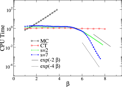
Figure 1: Temperature dependence of CPU time for equilibrium East model trajectories of total Monte Carlo time $t=10^{7}\times e^{2\beta}$ and system size $N=10^{5}$, for MC, CT, and MCAMC algorithms. The straight lines indicate the approximate speed-up of the MCAMC simulations. CPU time shown relative to the average time needed when using CT dynamics.

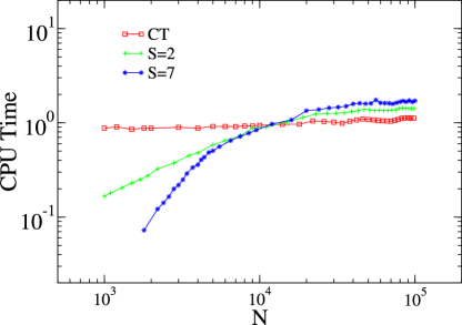
Figure 2: System size dependence of CPU time (relative to that for CT) for equilibrium East model trajectories of MC time $t=3\times 10^{12}/N$ at $T=0.2$.

As discussed above, the efficiency of MCAMC depends on the system size. In addition to a reduced time step this also determines the probability of encountering the isolated entry state for the $s>1$ algorithms. Fig. 2 shows the CPU time, now for different system sizes, at fixed temperature and total MC time $t=3\times 10^{12}/N$. Again, the CPU time for such a simulation using CT is constant. As expected, Fig. 2 shows that as $N$ becomes larger the MCAMC algorithms are less and less effective; beyond $N\epsilon^{2}\approx O(1)$ the CT scheme works better. This means that in order to maximise the MCAMC efficiency one needs to simulate the smallest possible system sizes. This is limited by the need to be compatible with bulk behaviour, which in the case of facilitated models requires that the system in average contains a sufficient number of excitations, i.e., $N\epsilon$ cannot be too small.

IX Example of results

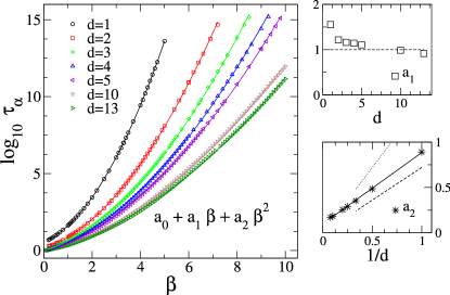
Figure 3: Persistence time $\tau_{\alpha}$ as a function of inverse temperature $\beta=1/T$ in the East model in dimensions $d=1-5,10,13$. The lines through the data points are quadratic fits, $\log\tau_{\alpha}=a_{0}+a_{1}\beta+a_{2}\beta^{2}$, with $a_{i}$ fitting parameters. The fit suggests that $a_{1}\sim 1$ in general. The bottom-right panel shows $a_{2}$ as a function of $d$. This coefficient seems to go as $a_{2}\approx b/d$, with the constant $b\approx 0.8$ (shown as a full line). This value is between $\ln 2$ (dotted line) and $(\ln 2)/2$ (dashed line).

In this section we present an example of numerical results obtained with the MCAMC.

A useful correlation function to study the relaxation of facilitated models is the persistence function $P(t)$, e.g. Buhot and Garrahan (2001); Garrahan and Chandler (2002); Berthier and Garrahan (2005), which gives the probability that a site has not changed its state up to time $t$. In terms of the local persistence field $p_{i}(t)=0,1$, where $1$ indicates that site $i$ has not flipped up to that time, and $0$ that it has flipped at least once, the persistence function reads $P(t)=N^{-1}\sum_{i}p_{i}(t)$. In contrast to standard MC or CT simulations, the MCAMC algorithm could run into problems when trying to measure persistence. By construction, it misses some of the events that could occur whilst in the transient subspace, for example, from the isolated state many spins could flip up and then flip back down before finally exiting to an absorbing state. At low temperatures in equilibrium, however, the contribution of these events is negligible, as the vast majority of changes to the global persistence function is from existing excitations spreading out into unmoved territory, and this is captured by the MCAMC algorithm. In fact, the only sites one needs to be concerned with are those immediately next to the initial excitations, which are very few in equilibrium at low $T$.

Figure 3 shows the equilibrium persistence time Garrahan and Chandler (2002); Berthier and Garrahan (2003), $\tau_{\alpha}$, of the East model in various dimensions $d$, calculated using the MCAMC algorithm with $s=2$. For all dimensions studied we find that $\tau_{\alpha}$ is a super-Arrhenius function of $T$. This seems to indicate that the East model is a fragile in all dimensions. Given that any simple mean-field estimate of the relaxation in this model would give Arrhenius behaviour, the above result would suggest that the East model has no upper critical dimension to its dynamics Garrahan and Chandler (2003). The data is compatible with $\log\tau_{\alpha}=a_{0}+a_{1}\beta+a_{2}\beta^{2}$, as expected if relaxation processes in the East model in any $d$ are quasi one-dimensional Garrahan and Chandler (2003). The coefficient $a_{2}$ of the quadratic fits is compatible with $a_{2}\approx b/d$ Garrahan and Chandler (2003), with the constant $b$ obeying $\ln 2\geq b\geq(\ln 2)/2$, reminiscent of the rigorous $d=1$ result of Ref. Aldous and Diaconis (2002). Note that the timescales reached with the MCAMC in Fig. 3 are between three and five orders of magnitude longer than in previous studies Berthier and Garrahan (2005).

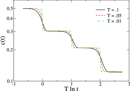
Figure 4: Concentration of excitations $c(t)$ as a function of scaled time $T\ln t$, in the $d=1$ East model after a quench from infinite temperature, from simulations with $s=7$ MCAMC.

The MCAMC proves also useful when simulating out-of-equilibrium dynamics. Consider the aging of the East model following a quench from infinite temperature. As the system relaxes towards its equilibrium the dynamics proceeds by stages characterized by the distance between isolated excitations Sollich and Evans (1999). These domains grow as $\overline{d}\sim t^{T\ln{2}}$. Consequently, the isolated transient state also plays an important role in such out-of-equilibrium dynamics of the East model, and the MCAMC algorithm is also applicable in this regime. Figure 4 shows the aging of the concentration of excitations, $c(t)$, with time after a quench to low temperatures in the East model, using the $s=7$ MCAMC algorithm.

In these aging simulations the nature of the speed-up due to the MCAMC becomes evident. Each stage of the dynamics is associated with an isolated domain of the form $10\cdots 0$. The $k$-th stage corresponds to domains of typical length $l\sim 2^{k}$, and a corresponding energy barrier of size $k$ to further relaxation Sollich and Evans (1999). In essence, at each successive plateau of $c(t)$ one requires an algorithm that produces time steps comparable to the activation time, $e^{k\beta}$. An $s=2$ MCAMC enables one to push simulations one plateau further than CT ($s=1$), the $s=7$ algorithm helps overcome the next energy barrier, and so on.

X Discussion

We have shown that the method of MC with absorbing Markov chains, MCAMC, of Novotny Novotny (1995) can be used to dramatically speed up simulations of facilitated spin models of glasses, such as the East and FA models. Even the simplest $s=2$ algorithm can improve simulation times at low temperature by a factor of $e^{2\beta}$ over the n-fold or continuous time MC. By increasing the number of transient states $s$ even larger computational gains can be achieved. One could imagine an algorithm where the number of transient states is variable, and at each iteration the $s$ with the largest number of transient states allowed by the current configuration, the smallest distance between excitations, is used.

The next future step would be to adapt MCAMC algorithms to other interesting KCMs, such as constrained lattice gases Kob and Andersen (1993); Jackle and Kronig (1994); Ritort and Sollich (2003); Toninelli et al. (2004); Pan et al. (2005); Lawlor et al. (2005) and $f$-spin facilitated FA models with $f>1$ Fredrickson and Andersen (1984); Ritort and Sollich (2003); Sellitto et al. (2005). Several features of these systems make the application of MCAMC less straightforward: since their kinetic constraints depend on more than one site, i.e. facilitation by two or more excitations in the FA models or two or more vacancies in the lattice gases, for generic entry states the tree of possible transient states is much larger than for, say, East models. This means that the computational cost of the necessary bookkeeping will be much higher (bookkeeping could be simplified by reducing the possible entry states, at the expense of triggering less frequently the MCAMC). This problem is compounded by the fact that $f>2$ FA models are very slow even at moderate temperatures, so that the potential exponential in $\beta$ gains from excitation rates are very modest, and may not even be enough to offset the bookkeeping cost—in constrained lattice gases, where barriers are purely entropic, this is bound to be worse. In any case, given that the high density or low temperature dynamics of these systems is in general so much slower than that of East models, a clever MCAMC algorithm which overcomes these hurdles could prove extremely useful.