Random field spin models beyond one loop: a mechanism for decreasing the lower critical dimension

Abstract

The functional RG for the random field and random anisotropy $O(N)$ sigma-models is studied to two loop. The ferromagnetic/disordered (F/D) transition fixed point is found to next order in $d=4+\epsilon$ for $N>N_{c}$ ($N_{c}=2.8347408$ for random field, $N_{c}=9.44121$ for random anisotropy). For $N<N_{c}$ the lower critical dimension $d=d_{\mathrm{lc}}$ plunges below $d_{\mathrm{lc}}=4$: we find two fixed points, one describing the quasi-ordered phase, the other is novel and describes the F/D transition. $d_{\mathrm{lc}}$ can be obtained in an $(N_{c}-N)$-expansion. The theory is also analyzed at large $N$ and a glassy regime is found.

It is important for numerous experiments to understand how the spontaneous ordering in a pure system is changed by quenched substrate impurities. One class of systems are modeled by elastic objects in random potentials (so-called random manifolds, RM). Another class are $O(N)$ classical spin models with ferromagnetic (Ferro) couplings in presence of random fields (RF) or anisotropies (RA). The latter describe amorphous magnets HarrisPlischkeZuckermann1973 . Examples of RF are liquid crystals in porous media FeldmanPelcovits2004 , He-3 in aerogels Matsumoto1997 , nematic elastomers FridrikhTerentjev1997 , and ferroelectrics Feldman2001 . The XY random field case $N=2$ is common to both classes and describes periodic RM such as charge density waves, Wigner crystals and vortex lattices BlatterFeigelmanGeshkenbeinLarkinVinokur1994 . Larkin showed Larkin1970 that the well-understood pure fixed points (FP) of both classes are perturbatively unstable to weak disorder for $d<d_{\mathrm{uc}}$ ($d_{\mathrm{uc}}=4$ in the generic case). For a continuous symmetry (i.e. the RF Heisenberg model) it was proven AizenmanWehr1989 that order is destroyed below $d=4$. This does not settle the difficult question of the lower critical dimension $d_{\mathrm{lc}}$ as a weak-disorder phase can survive below $d_{\mathrm{uc}}$, if associated to a non-trivial FP, as predicted in $d=3$ for the Bragg-glass phase with quasi long-range order (QLRO) GiamarchiLeDoussal1995 . For the random field Ising model $N=1$ (RFIM) it was argued ImryMa1975 , then proven Imbrie1984+BricmontKupiainen1987 that the ferromagnetic phase survives in $d=3$. Developing a field theory to predict $d_{\mathrm{lc}}$, and the exponents of the weak-disorder phase and the Ferro/Disordered (F/D) transition, has been a long-standing challenge. Both extensive numerics and experiments have not yet produced an unambiguous picture. Among the debated issues are the critical region of the 3D RFIM BelangerBookYoung+NattermannBookYoung and the possibility of a QLRO phase in amorphous magnets BarbaraCouachDieny1987 ; Fisch1998 ; Feldman2001 .

A peculiar property shared by both classes is that observables are identical to all orders to the corresponding ones in a $d-2$ thermal model AharonyImryShangkeng1976+EfetovLarkin1977+ParisiSourlas1979 . This dimensional reduction (DR) naively predicts $d_{\mathrm{lc}}=4$ for the weak-disorder phase in a RF with a continuum symmetry 16 and no Ferro order for the $d=3$ RFIM, which is proven wrong Imbrie1984+BricmontKupiainen1987 . It also predicts $d^{\mathrm{t}}_{\mathrm{uc}}=6$ for the F/D transition FP. While there is agreement that multiple local minima are responsible for DR failure, constructing the field theory beyond DR is a formidable challenge. Recent attempts include a reexamination of the $\phi^{4}$ theory (i.e. soft spins) for the F/D transition near $d=6$ BrezinDeDominicis . Previous large-$N$ approaches failed to find a non-trivial FP, but a self-consistent resummation including the $1/N$ corrections hinted at exponents different from DR (without succeeding in computing them) from a solution breaking replica symmetry MezardYoung1992 .

As for the pure $O(N)$ model, an alternative to the soft-spin version (near $d=6$) is the sigma model near the lower critical dimension (here presumed to be $d=4$). In 1985 D.S. Fisher Fisher1985b noticed that an infinite set of operators become relevant near $d=4$ in the RF $O(N)$ model. These were encoded in a single function $R(\phi)$ for which Functional RG equations (FRG) were derived to one loop, but no new FP was found. For a RM problem DSFisher1986 it was found that a cusp develops in the function $R(\phi)$ (the disorder correlator), a crucial feature which allows to obtain non-trivial exponents and evade DR. A fixed point for the RF model was later found GiamarchiLeDoussal1995 in $d=4-\epsilon$ for $N=2$. It was noticed only very recently Feldman2002 that the 1-loop FRG equations of Ref. Fisher1985b possess fixed points in $d=4+\epsilon$ for $N\geq 3$, providing a description of the long-sought critical exponents of the F/D transition.

In spite of these advances, many questions remain. Constructing FRG beyond one loop (and checking its internal consistency) is highly non-trivial. Progress was made for RM ChauveLeDoussalWiese2000a ; LeDoussalWiese2001 , and one hopes for extension to RF. Some questions necessitate a 2-loop treatment, e.g. for the depinning transition, as shown in LeDoussalWieseChauve2002 . In RF and RA models the 1-loop analysis predicted some repulsive FP in $d=4+\epsilon$ (for larger values of $N$), and some attractive ones GiamarchiLeDoussal1995 ; Feldman2000 in $d=4-\epsilon$. The overall picture thus suggests a lowering of the critical dimension, but how it occurs remains unclear. Finally the situation at large $N$ is also puzzling. Recently, via a truncation of exact RG TarjusTissier2004 it was claimed that DR is recovered for $N$ large.

Our aim in this Letter is twofold. We reexamine the overall scenario for the fixed points and phases of the $O(N)$ model using FRG. This requires the FRG to two loop. Here we present selected results, details are presented elsewhere LeDoussalWieseToBePublished . We find a novel mechanism for how the lower critical dimension is decreased below $d=4$ for $N<N_{c}$ at some critical value $N_{c}$. We obtain a description of the bifurcation which occurs at $N_{c}$, and below $N_{c}$ we find two perturbative FPs. Thanks to 2-loop terms $d_{\mathrm{lc}}$ can be computed in an expansion in $N_{c}-N$, and the Ferro/Para FP below $d=4$ is found. A study at large $N$ indicates that some glassy behavior survives there.

Let us consider $O(N)$ classical spins $\vec{n}(x)$ of unit norm $\vec{n}^{2}=1$. To describe disorder-averaged correlations one introduces replicas $\vec{n}_{a}(x)$, $a=1,\dots,k$, the limit $k=0$ being implicit everywhere. The starting model is a non-linear sigma model, of partition function ${\cal Z}=\int{\cal D}[\pi]\,{\mathrm{e}}^{-{\cal S}[\pi]}$ and action:

$${\cal S}[\pi]=\int{\mathrm{d}}^{d}x \Big{[} \!\frac{1}{2T_{0}}\sum_{a}[(\nabla\vec{\pi}_{a})^{2}+(\nabla\sigma_{a})^{2}]-\frac{1}{T_{0}}\sum_{a}M_{0}\sigma_{a}$$ (1)

$$-\frac{1}{2T_{0}^{2}}\sum_{ab}\hat{R}_{0}(\vec{n}_{a}\vec{n}_{b})\Big{]}\ ,$$

where $\vec{n}_{a}=(\sigma_{a},\vec{\pi}_{a})$ with $\sigma_{a}(x)=\sqrt{1-\vec{\pi}_{a}(x)^{2}}$. A small uniform external field $\sim M_{0}(1,\vec{0})$ acts as an infrared cutoff. Fluctuations around its direction are parameterized by $(N-1)$ $\pi$-modes. The ferromagnetic exchange produces the 1-replica part, while the random field yields the 2-replica term $\hat{R}_{0}(z)=z$ for a bare Gaussian RF. RA corresponds to $\hat{R}_{0}(z)=z^{2}$. As shown in Fisher1985b one must include a full function $\hat{R}_{0}(z)$, as it is generated under RG. It is marginal in $d=4$.

To obtain physics at large scales, one computes perturbatively the effective action $\Gamma[n_{a}(x)]$. It can be expanded in gradients near a uniform background configuration $n_{a}^{0}$, and splitted in 1-, 2- and higher-replica terms. From rotational invariance it is natural to look for $\Gamma$ in the form (1) with $\vec{n}_{a}\to\vec{n}_{a}^{R}=(\sigma_{a}^{R},\vec{\pi}_{a}^{R})$, $\sigma_{a}\to\sigma_{a}^{R}=\sqrt{1-(\pi_{a}^{R})^{2}}$, $\pi_{a}\to\pi_{a}^{R}=Z^{-1/2}\pi_{a}$, $T_{0}\to T_{R}=T_{0}/Z_{T}$, $M_{0}\to M_{R}=M_{0}\sqrt{Z}/Z_{T}$, $m=\sqrt{M_{R}}$ the renormalized mass of the $\vec{\pi}_{a}$ modes, and $\hat{R}_{0}(\vec{n}_{a}\vec{n}_{b})\to m^{\epsilon}\hat{R}(\vec{n}^{R}_{a}\vec{n}^{R}_{b})$. Higher vertices generated under RG are irrelevant by power-counting, hence discarded. Renormalization of $T$ contributes to the flow of $\hat{R}$, and one sets $T=0$ at the end.

One computes $Z$, $Z_{T}$ and $\hat{R}$ perturbatively in $\hat{R}_{0}$ and extracts $\beta$ and $\gamma$ functions $\beta[\hat{R}](z)=-m\partial_{m}\hat{R}(z)$, $\gamma=-m\partial_{m}\ln Z$ and $\gamma_{\mathrm{T}}=-m\partial_{m}\ln Z_{T}$, derivatives taken at fixed $\hat{R}_{0},T_{0},M_{0}$. Although calculation of the $Z$-factors is simplified due to DR, anomalous contributions appear from the non-analyticity of $\hat{R}(z)$. To compute $\hat{R}(z)$, one chooses a pair of uniform background fields $(n_{a}^{0},n_{b}^{0})$ for each $(a,b)$. We use a basis for the fluctuating fields (to be integrated over) such that ${\vec{n}}_{a}=(\sigma_{a},\eta_{a},\vec{\rho}_{a})$, ${\vec{n}}_{b}=(\sigma_{b},\eta_{b},\vec{\rho}_{b})$, where $\eta$ lies in the plane common to $(\vec{n}_{a}^{0},\vec{n}_{b}^{0})$, and $\vec{\rho}_{a}$ along the perpendicular $N-2$ directions; both have diagonal propagators. Denoting $\vec{n}_{a}^{0}\vec{n}_{b}^{0}=\cos\phi_{ab}$, one has $\vec{n}_{a}\vec{n}_{b}=\cos\phi_{ab}\left(\sigma_{a}\sigma_{b}+\eta_{a}\eta_{b}\right)+\sin\phi_{ab}\left(\sigma_{a}\eta_{b}-\sigma_{b}\eta_{a}\right)+\vec{\rho}_{a}\vec{\rho}_{b}$. One gets factors of $(N-2)$ from the contraction of $\vec{\rho}$. Our calculation to 2 loops results in the flow-equation for the function $R(\phi)=\hat{R}(z=\cos\phi)$, and $\epsilon=4-d$:

$$\partial_{\ell}R(\phi) = \epsilon R(\phi)+\frac{1}{2}R^{\prime\prime}(\phi)^{2}-R^{\prime\prime}(0)R^{\prime\prime}(\phi)+(N{-}2)\left[\frac{1}{2}\frac{R^{\prime}(\phi)^{2}}{\sin^{2}\phi}-\cot\phi R^{\prime}(\phi)R^{\prime\prime}(0)\right]$$ (2)

$$+\frac{1}{2}(R^{\prime\prime}(\phi)-R^{\prime\prime}(0))R^{\prime\prime\prime}(\phi)^{2}+(N{-}2)\bigg{[}\frac{\cot\phi}{\sin^{4}\phi}R^{\prime}(\phi)^{3}-\frac{5+\cos 2\phi}{4\sin^{4}\phi}R^{\prime}(\phi)^{2}R^{\prime\prime}(\phi)+\frac{1}{2\sin^{2}\phi}R^{\prime\prime}(\phi)^{3}$$

$$\qquad\qquad\qquad-\frac{1}{4\sin^{4}\phi}R^{\prime\prime}(0)\Big{(}2(2+\cos 2\phi)R^{\prime}(\phi)^{2}-6\sin 2\phi R^{\prime}(\phi)R^{\prime\prime}(\phi)+(5+\cos 2\phi)\sin^{2}\phi R^{\prime\prime}(\phi)^{2}\Big{)}\bigg{]}$$

$$-\frac{N{+}2}{8}R^{\prime\prime\prime}(0^{+})^{2}R^{\prime\prime}(\phi)-\frac{N{-}2}{4}\cot\phi R^{\prime\prime\prime}(0^{+})^{2}R^{\prime}(\phi)-2(N{-}2)\Big{[}R^{\prime\prime}(0)-R^{\prime\prime}(0)^{2}+\gamma_{a}R^{\prime\prime\prime}(0^{+})^{2}\Big{]}R(\phi)\qquad$$

with $\partial_{l}:=-m\partial_{m}$, and the last factor proportional to $R(\phi)$ is $-2\gamma_{\mathrm{T}}$ and takes into account the renormalization of temperature. Thanks to the anomalous terms, arising from a non-analytic $R(\phi)$, this $\beta$-function preserves a (at most) linear cusp (i.e. finite $R^{\prime\prime\prime}(0^{+})$), and reproduces for $N=2$ the previous 2-loop results for the periodic RM ChauveLeDoussalWiese2000a . For $N>2$, anomalous contributions are determined following LeDoussalWiese2005 . $\gamma$ is found as

$$\gamma=(N-1)R^{\prime\prime}(0)+{\textstyle\frac{3N-2}{8}}R^{\prime\prime\prime}(0^{+})^{2}\ ,$$ (3)

either via a calculation of $\langle\sigma_{a}\rangle$ , or of the mass corrections, a result consistent with the $\beta$ function (2) . The determination of $\gamma_{\mathrm{T}}$ is more delicate , and we have allowed for an amalous contribution $\gamma_{a}$, whose effect is minor, and discussed below. The correlation exponents (standard definition Feldman2002 ) are obtained as $\bar{\eta}=\epsilon-\gamma$, $\eta=\gamma_{\mathrm{T}}-\gamma$ at the FP. (2) has the form:

$$\partial_{\ell}R = \epsilon R+{\mathrm{B}}(R,R)+{\mathrm{C}}(R,R,R)+O(R^{4})$$ (4)

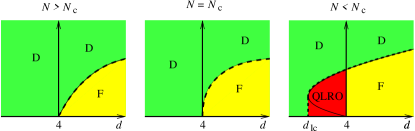
Figure 1: (Color online) Phase diagram. D $=$ disordered, F $=$ ferromagnetic, QLRO $=$ quasi long-range order.

We now discuss its solution, first in the RF case, and setting $\gamma_{a}=0$. The 1-loop flow-equation (setting $C=0$) admits, in dimensions larger than 4, a fixed point $R^{*}_{\mathrm{F/D}}$ with a single repulsive direction, argued by Feldman to describe the F/D zero temperature transition. This is true only for $N>N_{c}$. For $N<N_{c}$ this fixed point disappears and instead an attractive fixed point $R^{*}_{\mathrm{QLRO}}$ appears which describes the Bragg glass for $N=2$. We have determined $N_{c}=2.8347408$ and the solution $R_{c}(u)$ which satisfies $\mathrm{B}(R_{c},R_{c})|_{N=N_{c}}=0$. It is formally the solution at $\epsilon=0$. Since the FRG flow vanishes to one loop along the direction of $R_{c}$, examination of the 2-loop terms is needed to understand what happens at $N=N_{c}$. In particular the F/D transition should still exist for $N<N_{c}$, though it cannot be found at one loop. It is not even clear a priori whether it remains perturbative.

The scenario found is perturbative, accessible within a double expansion in $\sqrt{|\epsilon|}$ and $N-N_{c}$. To this aim, we write the leading terms in $N-N_{c}$ and $\epsilon$ of (4), namely

$$\!\!\!\partial_{\ell}R=\epsilon R+{\mathrm{B}}_{c}(R,R)+{\mathrm{C}}_{c}(R,R,R)+\left(N{-}N_{c}\right){\mathrm{B}}_{N}(R,R)$$

$$\!\!\!{\mathrm{B}}_{c}(\dots)=\mathrm{B}(\dots)|_{N=N_{c}}\ ,\qquad\!\!\!{\mathrm{C}}_{c}(\dots)=\mathrm{C}(\dots)|_{N=N_{c}}$$ (5)

One looks for a fixed-point solution of the form $R(u)=gR_{c}(u)+g^{2}\delta R(u)$, with $g>0$, $R_{c}^{\prime\prime}(0)=-1$, and its flow. This analysis is done numerically and leads to the flow shown schematically on Fig. 1. The RG-flow projected onto the direction of $g$ is equivalent to

$$\partial_{l}g = \epsilon g+1.092(N-N_{c})g^{2}+2.352g^{3}\ .$$ (6)

As a solution of the functional flow near $N_{c}$, its simplicity is surprising. Setting $g=(N_{c}-N)f$, there are three FP:

$$\frac{\epsilon}{(N-N_{c})^{2}}-1.092f+2.352f^{2}=0\ ,\quad\mbox{or}\quad f=0\ .\ \$$ (7)

Figure 2: (Color online) Parametric plot for solutions of (Random field spin models beyond one loop: a mechanism for decreasing the lower critical dimension) for $N<N_{c}$ (dots) for RF, equivalent to (6) (solid line, parabola) and flow (arrows). $f$ parameterizes disorder and only $f\geq 0$ is physical. Cmp. with fig. 1, right.

For $N>N_{c}$ the physical branch is $f<0$. As seen in Fig. 1, for $d>4$ there is a ferro phase (i.e. $f=0$ is attractive) and an unstable FP describing the F/D transition, given by the negative branch of (7). At $N=N_{c}$ one sees from (6) that the F/D fixed point is still perturbative, but in a $\sqrt{\epsilon}$ expansion for $g$ (and for the critical exponents). For $N<N_{c}$ the physical side is $f>0$ and there are two branches on Fig. 2 corresponding to two non-trivial fixed points. One is the infrared attractive FP for weak disorder which describes the Quasi-Ordered ferromagnetic phase; the second one is unstable and describes the transition to the disordered phase with a flow to strong coupling. These two fixed points exist only for $\epsilon<\epsilon_{c}$ and annihilate at $\epsilon_{c}$. The lower critical dimension of the RF-model for $N<N_{c}$ is lowered from $d=4$ to

$$d_{\mathrm{lc}}^{\mathrm{RF}}=4-\epsilon_{c}\approx 4-0.1268(N-N_{c})^{2}+O((N-N_{c})^{3})\ .$$ (8)

Note that the mechanism is different from the more conventional criterion $d-4+\eta(d)=0$ at $d=d_{\mathrm{lc}}$.

The same analysis for the random anisotropy class yields $N_{c}=9.44121$. The equivalent of (6) becomes $\partial_{l}g=\epsilon g+0.549(N-N_{c})g^{2}+47.6g^{3}$, leading to $d_{\mathrm{lc}}^{\mathrm{RA}}\approx 4-0.00158(N-N_{c})^{2}$. Although it yields $d_{\mathrm{lc}}(N=3)\approx 3.93$ and no QLRO phase in $d=3$, naive extrapolation should be taken with caution given the high value of $N_{c}$. Numerical values for $d_{\mathrm{lc}}$ are changed for a $\gamma_{a}\neq 0$, but the scenario is robust for $\gamma_{a}<\gamma_{c}$ .

We now discuss the FRG flow-equations for $N$ large. From a truncated exact RG Tarjus and Tissier (TT) TarjusTissier2004 found: that the linear cusp of the F/D fixed point for $d>4$ vanishes for $N>N^{*}(d)$, i.e. $R^{\prime\prime\prime}(0^{+})=0$; and that the non-analyticity becomes weaker as $N$ increases (as $|\phi|^{n}$ with $n\sim N$). Analytical study of the derivatives of (2) confirms the existence of this peculiar FP to two loop and predicts $N^{*}(d,2p)$ beyond which the set of $\{R^{(2k)}(0)\}$ for $k\leq p$ admits a stable FP, with $R^{(2k-1)}(0^{+})=0$ for $k\leq p$ and $R^{(2k-1)}(0^{+})\neq 0$ for $k>p$. We find:

$$N^{*}(d)=N^{*}(d,4)=18+49\epsilon/5+\dots$$ (9)

which yields a slope roughly twice the one of Fig. 1 of TarjusTissier2004 . This remarkable FP raises some puzzles. Although weaker than a cusp its non-analyticity should imply some (weaker) metastability in the system. It is thus unclear whether DR is fully restored: to prove it one should rule out feedback from anomalous higher-loop terms in exponents or the $\beta$-function. Finally, one also wonders about its basin of attraction. As shown in Fig. 3, the FRG flow for $R^{\prime\prime\prime\prime}(0)$ is still to large values if its bare value is large enough, indicating some tendency to glassy behaviour.

To explore these effects we now study the F/D phase transition at large $N$ and $d>4$. We obtain, both at large $N$ and fixed $d$ (extending Ref. LeDoussalWiese2001 ), and to one loop, the flow equation for the rescaled $\tilde{R}(z=\cos\phi)=NR(\phi)/|\epsilon|$:

$$\partial_{l}\tilde{R}=-\tilde{R}+2\tilde{R}_{1}^{\prime}\tilde{R}-\tilde{R}_{1}^{\prime}\tilde{R}^{\prime}z+{\textstyle\frac{1}{2}}\tilde{R}^{\prime 2}=0\ .$$ (10)

We denote $y(z)=\tilde{R}^{\prime}(z)$, $y_{0}=\tilde{R}^{\prime}(1)=-NR^{\prime\prime}(0)/|\epsilon|$ and $r_{4}=NR^{\prime\prime\prime\prime}(0)/|\epsilon|$. There are two analytic FPs $\tilde{R}(z)=z-1/2$ and $\tilde{R}(z)=z^{2}/2$, corresponding both to $y_{0}=1$ and to $r_{4}=1$ and $r_{4}=4$ respectively. This agrees with the flow of thed erivatives for analytic $R(\phi)$: $\partial_{l}y_{0}=y_{0}(y_{0}-1)$, and at $y_{0}=1$: $\partial_{l}r_{4}=\frac{1}{3}(r_{4}-1)(r_{4}-4)$. The first FP is the large-$N$ limit of the TT fixed point, the second is repulsive and divides the region where $r_{4}\to\infty$ (non-analytic $R(\phi)$) in a finite RG time $l_{c}$ (Larkin scale). For $y_{0}>1$, we find a family of NA fixed points with a linear cusp, parameterized by an integer $n\geq 2$, s.t. $y_{0}=n/(n-1)$, $z=y-(y_{0}-1)(y/y_{0})^{n}$. The solutions with $n$ (i.e. $z(y)$) odd correspond to random anisotropy ($R^{\prime}(\phi)=R^{\prime}(\phi+\pi)$). The $n=2$ RF fixed point is $R(\phi)=2\cos(\phi)+\frac{8\sqrt{2}}{3}\sin^{3}(\phi/2)-\frac{4}{3}$. To elucidate their role, we obtained the exact solution for the flow both below $l_{c}$, i.e. $z=\frac{y}{y_{0}}+(y_{0}-1)\Phi(\frac{y}{y_{0}})$ ($\Phi(x)$ parameterizes the bare disorder, $\Phi(1)=0$), and above $l_{c}$, with an anomalous flow for $y_{0}$. Matching at $l_{c}$ yields the critical manifold for RF disorder, defined from the conditions that $\Phi^{\prime}(w)=\Phi(w)/w=1$ has a root $0\leq w\leq 1$. It is different from the naive DR condition $y_{0}=1$, valid for small $r_{4}$. The $n=2$ FP corresponds to bare disorder such that the root $w=0$. Hence it is multicritical . Generic initial conditions within the critical F/P manifold flow back to the TT FP i.e. the linear cusp decreases to zero . This however occurs only at an infinite scale, hence we expect a long crossover within a glassy region, characterized by a cusp, and metastability on finite scales . The large-$N$ limit here is subtle. Taking $N\to\infty$ at fixed volume on a bare model with $\hat{R}_{0}(z)=z$ yields only the analytic FP, equivalent to a replica-symmetric saddle point. Higher monomials $z^{p}$ are generated in perturbation theory, at higher order in $1/N$. Thus, for $N$ large but fixed and infinite size, one must first coarse grain to generate a non-trivial function $\hat{R}_{0}(z)$, before taking the limit of $N\to\infty$.

In conclusion we obtained the 2-loop FRG functions for the random field and anisotropy $\sigma$-models. We found a new fixed point and a scenario for the decrease of the lower critical dimension. This rules out the scenario left open at one loop that the bifurcation close to $d=4$ simply occurs within the (quasi-) ordered phase.

Figure 3: Flow for $R^{\prime\prime\prime\prime}(0)/|\epsilon|$ for $d=4-\epsilon>4$ as a function of $N$. The two branches behave as $1/N$ and $4/N$ at large $N$.

References

- (1) R. Harris et al., Phys. Rev. Lett. 31 (1973) 60.
- (2) D.E. Feldman and R.A. Pelcovits, Phys. Rev. E 70 (2004) 040702.
- (3) K. Matsumoto et al., Phys. Rev. Lett. 79 (1997) 253.
- (4) S. V. Fridrikh and E. M. Terentjev, Phys. Rev. Lett. 79 (1997) 4661.
- (5) D.E. Feldman, Int. J. Mod. Phys. B 15 (2001) 2945.
- (6) G. Blatter et al., Rev. Mod. Phys. 66 (1994) 1125.
- (7) A.I. Larkin, Sov. Phys. JETP 31 (1970) 784.
- (8) M. Aizenman and J. Wehr, Phys. Rev. Lett. 62 (1989) 2503.
- (9) T. Giamarchi and P. Le Doussal, Phys. Rev. B 52 (1995) 1242.
- (10) Y. Imry and S.K. Ma, Phys. Rev. Lett. 355 (1975) 1399.
- (11) J.Z. Imbrie, Phys. Rev. Lett. 53 (1984) 1747; J. Bricmont and A. Kupiainen, Phys. Rev. Lett. 59 (1987) 1829.
- (12) D.P. Belanger, and T. Nattermann in A.P. Young, editor, Spin glasses and random fields, World Scientific, Singapore, 1997.
- (13) B. Barbara et al., Europhys. Lett. 3 (1987) 1129.
- (14) R. Fisch, Phys. Rev. B 58 (1998) 5684.
- (15) A. Aharony et al., Phys. Rev. Lett. 37 (1976) 1364; K.B. Efetov and A.I. Larkin, Sov. Phys. JETP 45 (1977) 1236; G. Parisi and N. Sourlas, Phys. Rev. Lett. 43 (1979) 744.
- (16) Early arguments in favor of a quasi-ordered phase for RA magnets in , see A. Aharony and E. Pytte, Phys. Rev. Lett. 45 (1980) 1583, also rely on a DR calculation.
- (17) E. Brezin and C. De Dominicis, Europhys. Lett. 44 (1998) 13, Eur. Phys. J. B 19 (2001) 467.
- (18) M. Mézard and P. Young, Eur. Phys. Lett. 18 (1992) 653.
- (19) D.S. Fisher, Phys. Rev. B 31 (1985) 7233.
- (20) D.S. Fisher, Phys. Rev. Lett. 56 (1986) 1964.
- (21) D.E. Feldman, Phys. Rev. Lett. 88 (2002) 177202.
- (22) P. Chauve et al., Phys. Rev. Lett. 86 (2001) 1785.
- (23) P. Le Doussal and K.J. Wiese, Phys. Rev. Lett. 89 (2002) 125702, Phys. Rev. B 68 (2003) 174202.
- (24) P. Le Doussal et al., Phys. Rev. B 66 (2002) 174201.
- (25) D.E. Feldman, Phys. Rev. B 61 (2000) 382.
- (26) G. Tarjus and M. Tissier, Phys. Rev. Lett. 93 (2004) 267008.
- (27) P. Le Doussal and K.J. Wiese, to be published.
- (28) P. Le Doussal and K.J. Wiese, Phys. Rev. E 68 (2005) 035101(R).
- (29) P. Le Doussal et al., Phys. Rev. E 69 (2004) 026112.