Quantum Spin Current Induced Through Optical Fields

Abstract

We propose a scheme to generate quantum spin current via optical dipole transition process. By coupling a three-level system based on the spin states of charged particles (electrons or holes in semiconductor) to the angular momentum states of the radiation, we show that a pure quantum spin current can be generated. No spin-orbit interaction is needed in this scheme. We also calculate the effect of nonmagnetic impurities on the created spin currents and show that the vertex correction of the spin hall conductivity in the ladder approximation is exactly zero.

Spintronics spintronics1 ; spintronics2 , the science and technology of manipulating the spin of the electron for building integrated information processing and storage devices, showed great promise and developed rapidly in recent years. In practical application, one of the most important goals is to create spin currents zhang ; niu . For this many interesting and basic phenomena, e.g. the spin hall effect niu ; hall1 ; hall2 in the system with spin-orbit coupling, have been discovered and further studied. On the other hand, spin currents can also be generated with the interference of two optical fields optical1 ; optical2 ; optical3 , or with optical Raman scattering effects sipe . Most of these methods in the generating quantum spin currents rely on the spin-orbit coupling such as Rashba coupling (caused by asymmetry of quantum well) and Dresselhaus term (induced by asymmetry of bulk crystal), etc. Moreover, coherent manipulation of spin states in semiconductor via optical dipole transitions has theoretically and experimentally been studied by many authors coherence1 ; coherence2 . With these ideas in mind, we propose here a new scheme to generate spin currents.

In this letter, we consider a realization of spin currents via optical dipole transition process in three-level system based on the spin states of the electrons (n-doped) or holes (p-doped) in semiconductor. The short-range scattering by the nonmagnetic impurities is discussed and the vertex correction of the spin hall conductivity is shown to be zero in the present optical model.

The three-level $\Lambda$-type system that we envisage for the scheme is given in Fig. 1. The system is confined to the two-dimensional $x-y$ plane with area $L_{x}\times L_{y}$ provided by the semiconductor quantum well. The particles in the system are subjected to an uniform electric field $\mathbb{E}$ in the $+x$ direction and a $+z$-directional uniform magnetic field ($\mathbb{B}_{0}=B_{0}\hat{\mathbb{e}}_{z}$) which can cause energy splitting and spin polarization in the $z$ direction ($S_{z}=s_{0},s_{+},s_{-}$, see Fig.1(a)). The transition $|s_{-}\rangle\rightarrow|s_{0}\rangle$ is coupled by a $\sigma_{+}$ light with the Rabi-frequency $\Omega_{1}=\Omega_{1}^{(0)}\exp(i\mathbb{k}_{1}\cdot\mathbb{r})$, where $\Omega^{(0)}_{1}(r)$ is the slowly spatially varying amplitude and $\mathbb{k}_{1}$ is the wave-vector. Another $\sigma_{-}$ light, characterized by the Rabi frequency $\Omega_{2}=\Omega^{(0)}_{2}(r)e^{i(l\phi+\mathbb{k}_{2}\cdot\mathbb{r})}$ with $\Omega^{(0)}_{2}(r)$ the slowly spatially varying amplitude, couples the transition $|s_{+}\rangle\rightarrow|s_{0}\rangle$, where $\phi=\tan^{-1}({y}/{x})$ and $\mathbb{k}_{2}$ is the wave-vector. $l$ indicates that the $\sigma_{-}$ photons are assumed to have the orbital angular momentum $\hbar l$ along the $+z$ direction.

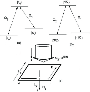
Figure 1: (a)$\Lambda$-type system based on spin states. (b) An example for dipole transitions in the $\Lambda$-type system provided by semiconductor GaAs quantum well, where the excited state $|1/2\rangle$ is a conduction band state, and the two ground states correspond to light-hole state (for $|-1/2\rangle$) and heavy-hole state (for $|3/2\rangle$), see ref.nonlinear and references therein. (c) Illustration of the two-dimensional system for present model.

As in previous works zhang ; niu ; hall2 ; nonlinear , we focus on the generation of spin current without particle-particle interaction. Defining the flip operators as $\hat{\sigma}_{\mu\nu}=|\mu\rangle\langle\nu|$ with energy levels $\mu,\nu=s_{0},s_{+},s_{-}$, the Hamiltonian in present system reads

$$H = H_{0}+H_{I}$$ (1)

$$H_{0} = \frac{1}{2m_{e}}(i\hbar\nabla_{xy}+e{\mathbb{A}}_{0})^{2}+V(x)-g_{s}\mu_{B}B_{0}S_{z}$$

$$H_{I} = -(\hbar\Omega_{2}\hat{\sigma}_{s_{0}s_{+}}+\hbar\Omega_{1}\hat{\sigma}_{s_{0}s_{-}})+h.c.,$$

where $\nabla_{xy}=\hat{\mathbb{e}}_{x}\partial_{x}+\hat{\mathbb{e}}_{y}\partial_{y}$, $V(x)=-eEx$ is the electric potential, parameters $e$, $m_{e}$, $\mu_{B}$ and $g_{s}$ represent the charge, the effective mass of a particle, Bohr magneton and Lande factor, respectively. ${\mathbb{A}}_{0}$ is the vector potential of the applied magnetic field, i.e. $B_{0}\hat{\mathbb{e}}_{z}=\nabla\times{\mathbb{A}}_{0}$. Note that spin-orbit interaction is not required in our model (we consider a very small or zero Rashba term in present case, see e.g. Rashba ). To facilitate the discussion, $H_{0}$ is written in $\mathbb{r}$-representation in eq (1). The interaction Hamiltonian $H_{I}$ can be diagonalized with the local unitary transformation: $\tilde{H}_{I}=U(\mathbb{r})H_{I}U^{{\dagger}}(\mathbb{r})$ with

$$U(\mathbb{r})={\left[\begin{matrix}\frac{1}{\sqrt{2}}&\frac{1}{\sqrt{2}}\sin\theta e^{-iS(\mathbb{r})}&\frac{1}{\sqrt{2}}\cos\theta\\ 0&\cos\theta&-\sin\theta e^{iS(\mathbb{r})}\\ \frac{1}{\sqrt{2}}&-\frac{1}{\sqrt{2}}\sin\theta e^{-iS(\mathbb{r})}&-\frac{1}{\sqrt{2}}\cos\theta&\end{matrix}\right]},$$ (2)

where $S=(\mathbb{k}_{2}-\mathbb{k}_{1})\cdot\mathbb{r}+l\phi$ and the mixing angle $\tan\theta(r)=|\Omega_{2}/\Omega_{1}|$. Under this unitary transformation, the three eigenstates of $H_{I}$ are easily obtained as $|\Psi_{\alpha}\rangle=\sum_{j=0,\pm}w^{(i)}_{j}|s_{j}\rangle$, where $\alpha=0,\pm$). The coefficients of these states are $w^{(0)}_{0}=0$, $w^{(0)}_{+}=\cos\theta$, $w^{(0)}_{-}=-\sin\theta$, $w^{(\pm)}_{0}=\frac{1}{\sqrt{2}},w^{(\pm)}_{+}=\pm\frac{1}{\sqrt{2}}\sin\theta$ and $w^{(\pm)}_{-}=\pm\frac{1}{\sqrt{2}}\cos\theta$, and the corresponding eigenvalues read $E^{(0)}=0,E^{(\pm)}=\pm\sqrt{|\Omega_{2}|^{2}+|\Omega_{1}|^{2}}$. Eigenstate $|\Psi_{0}\rangle$ is typically known as a dark state for a three-level $\Lambda$ system dark-state .

The Hamiltonian (1) can be rewritten in a covariant form with the definition of covariant derivative operator $\hat{\mathbb{D}}=-i\nabla-\mathbb{\tilde{A}}$, where $\mathbb{\tilde{A}}={\mathbb{A}}_{0}+{\mathbb{A}}_{e}$ is the sum of Abelian gauge potential ${\mathbb{A}}$ and the non-Abelian one ${\mathbb{A}}_{e}=-iU(\mathbb{r})\nabla U^{{\dagger}}(\mathbb{r})$, and the latter definition does not lead to the curvature term since it is a pure gauge. By a straightforward calculation, we find the $3\times 3$ matrix $\mathbb{\tilde{A}}$ has the following form:

$${\left[\begin{matrix}\frac{1}{\sqrt{2}}\sin^{2}\theta\nabla S+{\mathbb{A}}_{0}&(i\frac{1}{\sqrt{2}}\nabla\theta+\frac{1}{2\sqrt{2}}\sin 2\theta\nabla S)e^{-iS}&-\frac{1}{\sqrt{2}}\sin^{2}\theta\nabla S\\ (-i\frac{1}{\sqrt{2}}\nabla\theta+\frac{1}{2\sqrt{2}}\sin 2\theta\nabla S)e^{iS}&-\sin^{2}\theta\nabla S+{\mathbb{A}}_{0}&(i\frac{1}{\sqrt{2}}\nabla\theta-\frac{1}{2\sqrt{2}}\sin 2\theta\nabla S)e^{iS}\\ -\frac{1}{\sqrt{2}}\sin^{2}\theta\nabla S&(-i\frac{1}{\sqrt{2}}\nabla\theta-\frac{1}{2\sqrt{2}}\sin 2\theta\nabla S)e^{-iS}&\frac{1}{\sqrt{2}}\sin^{2}\theta\nabla S+{\mathbb{A}}_{0}\end{matrix}\right]}$$ (3)

which generally is a $SU(3)$ non-Abelian gauge potential. The off-diagonal matrix elements of it represent the transitions between each two of $|\Psi_{0}\rangle$ and $|\Psi_{\pm}\rangle$. However, considering the present system is non-degenerate, we can introduce the adiabatic approximation when both light fields vary sufficiently slowly in space. For a numerical estimate, we consider the case $|\frac{\Omega_{2}}{\Omega_{1}}|=\lambda\rho\propto\rho$ where $\lambda$ is constant and $\rho=\sqrt{x^{2}+y^{2}}$ the distance from $z$ axis ohberg . The typical values can be taken as coherence1 : $\Omega_{0}^{2}=(\Omega_{1}^{2}+\Omega_{2}^{2})^{1/2}\sim 10ps^{-1}$, $l\leq 10^{4}$, $\lambda\sim 10^{4}m^{-1}$ and the radius of the interaction region in the $x-y$ plane is $R\sim 1.0cm$, the transition rate can then be evaluated as $\Gamma_{ab}<10^{-3}\ll 1$ for any two different states ($a\neq b=\pm,0$). Thus we neglect the off-diagonal matrix elements in eq.(3) and yield a nontrivial adiabatic gauge connection $\mathbb{\tilde{A}}\rightarrow\mathbb{\tilde{A}^{diag}}$, which is associated with a $3\times 3$ diagonal matrix for the magnetic field with each component ($B_{k}=\frac{1}{2}\epsilon_{kmn}F_{mn}=\frac{\hbar}{2}\epsilon_{kmn}[\hat{D}_{m},\hat{D}_{n}]$)

$$\mathbb{B}_{11}=\mathbb{B}_{33}=(B_{0}+B_{e})\hat{\mathbb{e}}_{z},\ \ \ \mathbb{B}_{22}=(B_{0}-2B_{e})\hat{\mathbb{e}}_{z}$$ (4)

where $B_{e}=\hbar l\lambda^{2}/e$ indicates the strength of additional effective magnetic fields induced by the optical fields depends on the angular momentum $\hbar l$ that can have a large value from a vortex optical beam angular . For our present purpose we choose $B_{0}=B_{e}/2$ so that $B_{11}^{z}=B_{33}^{z}=-B_{22}^{z}=3\hbar l\lambda^{2}/2e$. In this case, we obtain an interesting result that the $z$ component of $\mathbb{B}_{22}$ is opposite to that of $\mathbb{B}_{11}$ (and of $\mathbb{B}_{33}$) (see fig.2(a) and (b)), a key point for realizing quantum spin current.

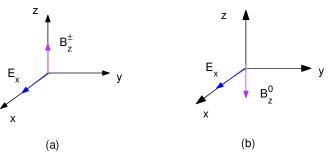
Figure 2: (color online) (a)(b) Schematic illustration of the electric field and the effective magnetic field, where $\mathbb{B}^{0}=\mathbb{B}_{22},\mathbb{B}^{+}=\mathbb{B}^{11}$ and $\mathbb{B}^{-}=\mathbb{B}^{33}$.

Up to this point, the interaction Hamiltonian is diagonal and we can rewrite $H$ in eq.(1) in the following effective form:

$$H_{eff}=\frac{\hbar^{2}}{2m_{e}}\hat{D}^{2}+\tilde{V}(\mathbb{r}),$$ (5)

where $\tilde{V}(\mathbb{r})=\bigr{(}U(\mathbb{r})VU(\mathbb{r})\bigr{)}^{diag}$ is a $3\times 3$ diagonal matrix with its elements $\tilde{V}_{11}=\tilde{V}_{22}+\Omega_{0},\tilde{V}_{22}=V(x)-g_{s}\mu_{B}B_{0}S_{z}$ and $\tilde{V}_{11}=\tilde{V}_{22}-\Omega_{0}$. The momentum operator is defined by $\hat{\mathbb{p}}=-i\hbar\hat{\mathbb{D}}$ and it has the nontrivial communication relations: $[r_{i},\hat{p}_{j}]=i\hbar\delta_{ij},[r_{i},r_{j}]=0,[\hat{p}_{i},\hat{p}_{j}]=-i\hbar F_{ij}$. Generally the dynamics of this situation is determined by the $SU(3)$ gauge symmetry. By considering adiabatic condition, the transitions between any two of the states $|\Psi_{\alpha}\rangle(\alpha=0,\pm)$ can be neglected and the symmetry $SU(3)$ readily reduces to an Abelian one: $SU(3)\rightarrow U(1)\otimes U(1)\otimes U(1)$. The quantum state of each particle can be expanded by the complete eigenbasis of the interaction Hamiltonian $|\mathbb{\Psi}\rangle=\sum_{\alpha=0,\pm}\Phi_{\alpha}|\Psi_{\alpha}\rangle$, where the coefficients $\Phi_{\alpha}$ can be determined by the initial conditions. Note that each eigenstate $|\Psi_{\alpha}\rangle$ consists of different spin states $|s_{0}\rangle$ and $|s_{\pm}\rangle$. However, since $|\Psi_{\alpha}\rangle$ are eigenstates of the interaction Hamiltonian $H_{I}$, and $H_{0}$ does not lead to the transition between $|s_{0}\rangle$ and $|s_{\pm}\rangle$, the expectation value of the $z$-axis spin polarization of any state $|\Psi_{\alpha}\rangle$ is time-independent. Therefore, for convenience, we can treat the states $|\Psi_{\alpha}\rangle$ approximately as new “effective spin states” with their $z$-axis spin polarization calculated by $S_{z}^{\alpha}=\langle\Psi_{\alpha}|S_{z}|\Psi_{\alpha}\rangle$. It is easy to see that $S_{z}^{(0)}=\cos^{2}\theta s_{+}+\sin^{2}\theta s_{-}$, $S_{z}^{(+)}=S_{z}^{(-)}=\frac{1}{2}s_{0}+\frac{1}{2}(\sin^{2}\theta s_{+}+\cos^{2}\theta s_{-})$. Since the particles in different effective spin states $|\Psi_{\alpha}\rangle$ experience different effective magnetic fields, they may move in opposite directions depending on the index $\alpha$, generating a spin current.

To facilitate the subsequent calculations, we note that the particles with effective spin state $|\Psi_{\alpha}\rangle(\alpha=0,\pm)$ interact with the magnetic field $\mathbb{B}^{\alpha}$ where $\mathbb{B}^{0}=\mathbb{B}_{22}$ and $\mathbb{B}^{\pm}=\mathbb{B}_{11}=\mathbb{B}_{33}$. It is convenient to choose the diagonal-elements of the gauge connection $\mathbb{\tilde{A}}(\mathbb{r})$ as $\mathbb{\tilde{A}}_{\alpha}=\frac{e}{c}B^{\alpha}_{z}x\hat{e}_{y}$, so that $p^{\alpha}_{y}=k$ is a good quantum number. With the definition $\hat{a}_{\alpha k}=\frac{1}{\sqrt{2}l_{B}}\bigr{[}(x-\frac{Ec}{B\omega})+(-\frac{k}{B^{\alpha}}+i\frac{p_{x}}{B})\frac{c}{e}\bigr{]}$ where $B=|B^{\alpha}|=3B_{e}/2$ and $l_{B}=\sqrt{\hbar c/eB}$, the Hamiltonian for a given $k$ can further be rewritten as

$$H_{eff}=\hbar\omega\bigr{(}\hat{a}^{{\dagger}}_{\alpha k}\hat{a}_{\alpha k}+\frac{1}{2}\bigr{)}-gB_{0}S_{z}^{\alpha}+H_{c},$$ (6)

where $H_{c}=-\frac{E_{x}^{2}}{2B^{2}}mc^{2}-\frac{E_{x}}{B^{\alpha}_{z}}kc$, $g=g_{s}\mu_{B}$ and $\omega=\frac{eB}{m_{e}c}$. Operators $\hat{a}_{\alpha k}$ satisfy the communication relation $[\hat{a}_{\alpha k},a^{{\dagger}}_{\beta k^{\prime}}]=\delta_{\alpha\beta}\delta_{kk^{\prime}}$. The eigenstate of above Hamiltonian can be written as $|n,k,\alpha\rangle$ with its eigenvalue $\epsilon_{n,k,\alpha}=(n+1/2)\hbar\omega-gB_{0}S_{z}^{\alpha}+H_{c}$. The analytical results allow us to calculate the charge and spin current. The spin current operator for a single particle is defined by $j^{s_{z}}_{s}=\frac{\hbar}{2}(S_{z}v_{y}+v_{y}S_{z})$, where $v_{y}=[y,H]/i\hbar=p_{y}+x\omega$ is the velocity operator in the $y$ direction hall2 and the corresponding charge current operator reads $j_{c}=ev_{y}$.

With the above definitions, for a $N_{e}$-particle system the average current density can be calculated by

$$J^{s_{z}}_{c,y}=\frac{1}{L_{x}}\sum_{n,k,\alpha}(j^{s_{z}}_{c,y})_{nk}f(\epsilon_{n,k,\alpha}).$$ (7)

where $(j^{s_{z}}_{c,y})_{nk}=\sum_{\alpha}\langle n,k,\alpha|j^{s_{z}}_{c,y}|n,k,\alpha\rangle$ is the current carried by one particle in the state $|n,k\rangle$. $f(\epsilon_{n,k,\alpha})$ is the Fermi distribution function, and $N_{e}=\sum_{n,k,\alpha}f(\epsilon_{n,k,\alpha})$. When the coefficient $\Phi_{\alpha}$ of the initial state takes on the simple value $|\Phi_{0}|^{2}=1/2$, $|\Phi_{+}|^{2}=\cos^{2}\gamma/2$ and $|\Phi_{-}|^{2}=\sin^{2}\gamma/2$, a pure spin current is obtained by

$$(j^{s_{z}}_{y})_{nk}=\frac{eE_{x}}{6\hbar l\lambda^{2}}\bigr{(}\cos 2\theta(s_{+}-s_{-})-s_{0}\bigr{)},\ \ j_{c}=0.$$ (8)

The spin current in above equation is dependent on the space position $(x,y)$. This is because the effective spin polarization of the state $|\Psi_{\alpha}\rangle$ is dependent on space (see Fig. 3). Together with the Eq. (7) we further calculate the average spin current

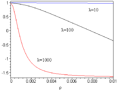
Figure 3: (color online) Space spreading of generated spin current versus the unit $\frac{eE_{x}}{9\hbar l\lambda^{2}}$, where $\lambda=10(1/m)$ for the blue line, $\lambda=100(1/m)$ for the black line and $\lambda=1000(1/m)$ for the red line. $\rho=\sqrt{x^{2}+y^{2}}$ versus the unit $m$.

$$J^{s_{z}}_{y}=\frac{eE_{x}n_{e}}{6\hbar l\lambda^{2}}\bigl{(}4s_{\pm}\frac{\tan^{-1}\bigr{(}\lambda L_{x}/2\sqrt{1+\lambda^{2}y^{2}}\bigr{)}}{\lambda L_{x}\sqrt{1+\lambda^{2}y^{2}}}-s_{\pm}-s_{0}\bigr{)},$$ (9)

where $s_{\pm}=s_{+}-s_{-}$, and $n_{e}$ is the filling of charged particles (unit $1/m^{2}$). It is interesting that generally the average spin current is still dependent on the position $y$. For practical application, here we consider the case that the $\lambda L_{x}\gg 1$, i.e. the $\sigma_{-}$ field is much stronger than $\sigma_{+}$ one. Then from the Eq. (9) we obtain the persistent spin current $J^{s_{z}}_{y}=-\frac{eE_{x}n_{e}}{6\hbar l\lambda^{2}}(s_{\pm}+s_{0})$. To provide some numerical evaluations, we set hall2 ; coherence1 $n_{e}=1.0\times 10^{16}/m^{2},l\lambda^{2}=3.0\times 10^{13}/m^{2}$ ($\lambda L_{x}\gg 1$) and the spin polarization $s_{+}=3\hbar/2,s_{-}=-\hbar/2,s_{0}=\hbar/2$ (fig.1(b)). For these values, we obtain the spin hall conductivity $\sigma_{yx}^{s}=J^{s_{z}}_{y}/E_{x}\approx 1.38\times 10^{2}$e. The above result can be understood as follow: from the formula of $H_{c}$ one can find the particles in the effective spin state $|\Psi_{\alpha}\rangle$ have a group velocity $\mathbb{v}^{\alpha}=-E_{x}/B^{\alpha}_{z}\hat{e}_{y}$ in the $y$ direction. As in present case $B^{+}=B^{-}=-B^{0}$, the group velocities $v^{+}=v^{-}=-v^{0}$. Therefore, a pure dissipationless spin current can be generated when the particles have the same probability in state $|\Psi_{0}\rangle$ with the sum of $|\Psi_{+}\rangle$ and $|\Psi_{-}\rangle$. It should be pointed out that, for GaAs quantum well, this numerical evaluation should be revised by a constant factor, because another independent three-level system ($s^{\prime}_{+}=\hbar/2,s^{\prime}_{-}=-3\hbar/2,s^{\prime}_{0}=-\hbar/2$, noted by $\Lambda^{\prime}$ system) can also interact with the optical fields besides the one shown in fig.1(b) nonlinear1 . If we neglect the detunings of the optical transitions and according to $s^{\prime}_{\pm}+s^{\prime}_{0}=3\hbar/2<s_{\pm}+s_{0}$, the $\Lambda^{\prime}$ system will slightly decrease the present generated spin currents.

By now all the discussions are based on a clean semiconductor system. Noting that the vertex correction may remarkably cancel the spin hall currents in Rashba system when the s-wave impurity scattering is considered vertex1 ; vertex2 , it is much suggestive to discuss such effect in the present model. For this we consider the following short-range nonmagnetic impurity Hamiltonian:

$$H_{imp}=\sum_{j}u\delta(\mathbb{r}-\mathbb{R}_{j}).$$ (10)

The free retarded Green’s function $G_{R}^{(0)}(\epsilon,k)=[\epsilon-H_{eff}]^{-1}$ is diagonal in the effective spin space:

$$G_{R;n,\alpha}^{(0)}(\epsilon,k)=\frac{1}{\epsilon-\epsilon_{n,k,\alpha}+i\eta}\delta_{nn^{\prime}}\delta_{\alpha\alpha^{\prime}}.$$ (11)

In the Born approximation, the self-energy related to free green function in our system can be calculated by $\Sigma^{R}(\epsilon)=n_{imp}u^{2}\int\mathcal{N}_{e}(\epsilon_{n,k,\alpha})G_{R;n,\alpha}^{(0)}(\epsilon,k)d\epsilon_{n,k,\alpha}$, where $n_{imp}$ is the impurity density and $\mathcal{N}_{e}(\epsilon_{n,k,\alpha})$ the electron state density. It can be verified that $\Sigma^{R}(\epsilon)=-i\pi n_{imp}u^{2}\mathcal{N}_{e}(\epsilon)$, thus the total Green’s function reads $G_{R;n,\alpha}(\epsilon,k)=\frac{1}{\epsilon-\epsilon_{n,k,\alpha}+i/2\tau}\delta_{nn^{\prime}}\delta_{\alpha\alpha^{\prime}}$. Here $\tau=2\pi n_{imp}u^{2}\mathcal{N}_{e}$ represents the mean scattering free time. With these results we calculate the vertex correction of charge current $j_{\alpha,x}^{vertex}$ in the ladder approximation as

$$\sum_{n,\alpha}\frac{1}{2\pi\tau\mathcal{N}_{e}}\int\frac{dk}{2\pi}G_{A;n,\alpha}(\epsilon,k)j_{\alpha,x}G_{R;n,\alpha}(\epsilon,k) = \sum_{n,\alpha}\frac{e}{2\pi m\tau\mathcal{N}_{e}}\biggr{(}\int\frac{dk}{2\pi}G_{A;n,\alpha}(\epsilon,k)\sqrt{\frac{eB\hbar}{2c}}\bigr{(}\sqrt{n+1}\delta_{n,n^{\prime}-1}+$$ (12)

$$+\sqrt{n}\delta_{n,n^{\prime}+1}\bigr{)}G_{R;n,\alpha}(\epsilon,k)\biggr{)},$$

where the advanced Green’s function $G_{A;n,\alpha}(\epsilon,k)=\{G_{R;n,\alpha}(\epsilon,k)\}^{*}$. Notice that the Green’s function in the present system is diagonal in both Landau level and effective spin space: $G^{A,R}_{n,\alpha}(\epsilon,k)\propto\delta_{nn^{\prime}}\delta_{\alpha\alpha^{\prime}}$, whereas integral function in the right-hand side of above equation is also proportional to $\delta_{n,n^{\prime}+1}$ or $\delta_{n,n^{\prime}-1}$, the vertex correction of charge current in ladder approximation is exactly zero. When we turn to the ladder diagrams of the spin Hall conductivity $\sigma_{yx}^{s}$, we have to take into account the vertex correction in the charge current only vertex1 . Therefore, because of this vanishing vertex correction, the spin current obtained in our optical method reproduces its value obtained from a clean system without impurities from the outset.

Finally, we present an experimental realization of the initial condition required for the result in eq. (7). Firstly, we can trap the system in dark state using two light fields with equal Rabi-frequencies (i.e. $|\Omega_{1}|=|\Omega_{2}|$) and switch both lights off simultaneously, hence the state $|\Psi(t_{0})\rangle=(|s_{+}\rangle-|s_{-}\rangle)/\sqrt{2}$. In this step no angular momentum is needed for the $\sigma_{-}$ light field. Secondly, we only turn the $\sigma_{+}$ light on again. Meanwhile the population in the state $|s_{+}\rangle$ keeps $1/2$ unchanged while the state $|s_{-}\rangle$ is coupled to the state $|s_{0}\rangle$ by the $\sigma_{+}$ light and the state reads $|\Psi(t_{1})\rangle=(\sin|\Omega_{1}|(t_{1}-t_{0})|s_{0}\rangle+\cos|\Omega_{1}|(t_{1}-t_{0})|s_{-}\rangle+|s_{+}\rangle/)\sqrt{2}$. Thirdly, we adiabatically turn on the $\sigma_{-}$ light field with $z$-directional angular momentum and arrive at the adiabatic evolution of the state $|\Psi(t)\rangle=\frac{1}{\sqrt{2}}\bigr{(}\frac{1}{\sqrt{2}}e^{-i\gamma t}|\Psi_{+}\rangle-\frac{1}{\sqrt{2}}e^{i\gamma t}|\Psi_{-}\rangle+|\Psi_{0}\rangle\bigr{)}$ where $\gamma=\int_{t_{0}}^{t}\sqrt{|\Omega_{1}|^{2}+|\Omega_{2}|^{2}}dt$. Obviously, this is the state needed for the initial condition.

In practice, the spreading of light fields have a boundary in the $x$-$y$ plane which may lead to modification in the Landau energy levels. However, based on the previous results ohberg , this boundary effect can be safely neglected when $l\lambda^{2}L_{x}L_{y}\gg 1$, which is achieved using a light beam with a large angular momentum. On the other hand, we should emphasize that the particle-particle interaction may lead to a renormalization of the Rabi-frequencies $\Omega_{1,2}$ of the transitions between states $|s_{0}\rangle$ and $|s_{\pm}\rangle$ coupled by the light fields nonlinear1 ; nonlinear2 . However for simplicity, as in previous works zhang ; niu ; hall2 ; nonlinear , we do not need to consider such effects in the present model. All these interesting aspects will be further discussed in future publications. In conclusion, we have proposed and demonstrated a means of generating quantum spin current optical dipole transition process. The short-range scattering by the nonmagnetic impurities are discussed and the vertex correction of the spin hall conductivity is shown to be zero in the present optical model.

We thank Prof Mansoor B. A. Jalil, S. -Q. Gong and Dr S. G. Tan for valuable discussions. This work is supported by NUS academic research Grant No. WBS: R-144-000-172-101, and by NSF of China under grants No.10275036.

References

(1) S. A. Wolf, et al., Science 294, 1488 (2001);
I. Zutic and S. D. Sarma, Rev. Mod. Phys. 76,323 (2004).
(2) Semiconductor Spintronics and Quantum Computation,
edited by D. Awschalom, D. Loss and N. Samarth (Springer, Berlin, 2002).
(3) S. Murakami, N. Nagaosa, S.-C. Zhang, Science 301, 1348 (2003); Phys. Rev. B 69,235206 (2004).
Z. F. Jiang, R. D. Li, S.-C. Zhang and W. M. Liu, Phys. Rev. B 72,
045201 (2005).
(4) J. Sinova, D. Culcer, Q. Niu, N. A. Sinitsyn, T. Jungwirth and A.H. MacDonald
Phys. Rev. Lett. 92, 126603 (2004); Y. K. Kato et al., Science, 306, 1910 (2004).
(5) B. K. Nikolić, S. Souma, Liviu P. Zârbo and J. Sinova, Phys. Rev. Lett. 95, 046601 (2005);
J. Wunderlich et al., Phys. Rev. Lett. 94, 047204 (2005).
(6) S. -Q. Shen, Michael Ma, X. C Xie and F. C. Zhang Phys. Rev. Lett. 92, 256603
(2004); S. Murakami, N. Nagaosa and S.-C. Zhang, Phys. Rev. Lett.
93, 156804 (2004).
(7) M. J. Stevens, Arthur L. Smirl, R. D. R. Bhat, Ali
Najmaie, J. E. Sipe, and H. M. van Driel, Phys. Rev. Lett. 90,
136603 (2003); J. Hübner et al., Phys. Rev. Lett. 90, 216601
(2003).
(8) E. Ya. Sherman, A. Najmaie and J. E. Sipe,
Appl. Phys. Lett. 86, 122103 (2005); R. D. R. Bhat, et al., Phys.
Rev. Lett. 94, 096603 (2005).
(9) S. D. Ganichev et al., J. Phys. Condens.
Matter 15, R935 (2003).
(10) A. Najmaie, E. Y. Sherman and J. E. Sipe, Phys. Rev. Lett. 95,056601 (2005);
Phys. Rev. B 72,041304(R) (2005).
(11) A. Imamoglu et al., Opt. Lett. 19, 1744
(1994); G. S. Agarwal, Phys. Rev. A 51, R2711 (1995); G. B.
Serapiglia et al., Phys. Rev. Lett. 84, 1019 (2000).
(12) M. Phillips and H. Wang, Phys. Rev. Lett. 89,
186401 (2002); K.-M. C. Fu et al., Phys. Rev. Lett. 95, 187405
(2005).
(13) X. Zhu, M. S. Hybertsen and P. B. Littlewood, Phys.
Rev. B 50,11915 (1994).
(14) J. Nitta, et al., Phys. Rev. Lett. 78,1335
(1997); M. M. Glazov, et al., Phys. Rev. B 71, 241312(R) (2005),
and references therein.
(15) S.E.Harris, Phys. Today, 50,36(1997); Xiong-Jun Liu, Hui Jing, Xin
Liu and Mo-Lin Ge, Phys. Lett. A 355, 437 (2006).
(16) G.Juzeliūnas et al., Phys. Rev. Lett. 93, 033602(2004).
(17) J. Ruseckas, et al., Phys. Rev. Lett. 010404 (2005).
(18) J. Inoue, G. E.W. Bauer, and L.W. Molenkamp, Phys. Rev. B 67, 033104
(2003); Phys. Rev. B 70, 041303(R) (2004); cond-mat/0402442; S.
Murakami, Phys. Rev. B 69, 241202(R) (2004).
(19) J. Schliemann and D. Loss, Phys. Rev. B 69, 165315
(2004); A. A. Burkov and A. H. MacDonald, Phys. Rev. B 70, 155308
(2004).
(20) M. Lindberg and R. Binger, Phys. Rev. Lett.
75, 1403 (1995); R. Binger and M. Lindberg, Phys. Rev. B 61, 2830
(2000).
(21) H. Huang and S. W. Koch, Quantum Theory of
the Optical and Electronic Properties of Semiconductors (World
Scientific, Singapore, 1993), 2nd ed.