The Mechanical Threshold Stress model for various tempers of AISI 4340 steel

Abstract

Numerical simulations of high-strain-rate and high-temperature deformation of pure metals and alloys require realistic plastic constitutive models. Empirical models include the widely used Johnson-Cook model and the semi-empirical Steinberg-Cochran-Guinan-Lund model. Physically based models such as the Zerilli-Armstrong model, the Mechanical Threshold Stress model, and the Preston-Tonks-Wallace model are also coming into wide use. In this paper, we determine the Mechanical Threshold Stress model parameters for various tempers of AISI 4340 steel using experimental data from the open literature. We also compare stress-strain curves and Taylor impact test profiles predicted by the Mechanical Threshold Stress model with those from the Johnson-Cook model for 4340 steel. Relevant temperature- and pressure-dependent shear modulus models, melting temperature models, a specific heat model, and an equation of state for 4340 steel are discussed and their parameters are presented.

1 Introduction

The present work was motivated by the need to simulate numerically the deformation and fragmentation of a heated AISI 4340 steel cylinder loaded by explosive deflagration. Such simulations require a plastic constitutive model that is valid over temperatures ranging from 250 K to 1300 K and over strain rates ranging from quasistatic to the order of $10^{5}$ /s. The Mechanical Threshold Stress (MTS) model (Follansbee and Kocks [14], Kocks [29]) is a physically-based model that can be used for the range of temperatures and strain rates of interest in these simulations. In the absence of any MTS models specifically for 4340 steels, an existing MTS model for HY-100 steel (Goto et al. [16, 17]) was initially explored as a surrogate for 4340 steel. However, the HY-100 model failed to produce results that were in agreement with experimental stress-strain data for 4340 steel. This paper attempts to redress that issue by providing the MTS parameters for a number of tempers of 4340 steel (classified by their Rockwell C hardness number). The MTS model is compared with the Johnson-Cook (JC) model (Johnson and Cook [25, 26]) for 4340 steel and the relative advantages and disadvantages of these models are discussed.

The MTS model requires a temperature and pressure dependent elastic shear modulus. We describe a number of shear modulus models and the associated melting temperature models. Conversion of plastic work into heat is achieved through a specific heat model that takes the transformation from the bcc ($\alpha$) phase to the fcc ($\gamma$) phase into account. The associated Mie-Grüneisen equation of state for the pressure is also discussed.

The organization of this paper is as follows. For completeness we provide brief descriptions of the models used in this paper in Section  2. Parameters for the submodels required by the MTS model (for example, the shear modulus model) are determined and validated in Section 3. Details of the procedure used to determine the MTS model parameters are given in Section 4. Predictions from the MTS model are compared with those from the Johnson-Cook model in Section 5. These comparisons include both stress-strain curves and Taylor impact tests. Conclusions and final remarks are presented in Section 7.

2 Models

In this section, we describe the form of the MTS plastic flow stress model and the associated submodels for the specific heat, melting temperature, shear modulus, and the equation of state that have have used for the computations in this paper. The submodels are used during the stress update step in elastic-plastic numerical computations at high strain rates and high temperatures. The submodels discussed in this paper are:

1. Specific Heat: the Lederman-Salamon-Shacklette model.

2. Melting Temperature: the Steinberg-Cochran-Guinan (SCG) model and the Burakovsky-Preston-Silbar (BPS) model.

3. Shear Modulus: the Varshni-Chen-Gray model (referred to as the MTS shear modulus model in this paper), the Steinberg-Cochran-Guinan (SCG) model, and the Nadal-LePoac (NP) model.

4. Equation of State: the Mie-Grüneisen model.

More details about the models may be found in the cited references.

The following notation has been used uniformly in the equations that follow.

$$\dot{\epsilon} =~{}\text{Strain rate}$$

$$\epsilon_{p} =~{}\text{Plastic strain}$$

$$\mu =~{}\text{Shear modulus}$$

$$\rho =~{}\text{Current mass density}$$

$$\rho_{0} =~{}\text{Initial mass density}$$

$$\eta=\rho/\rho_{0} =~{}\text{Compression}$$

$$\sigma_{y} =~{}\text{Yield Stress}$$

$$b =~{}\text{Magnitude of the Burgers vector}$$

$$k_{b} =~{}\text{Boltzmann constant}$$

$$p =~{}\text{Pressure (positive in compression)}$$

$$C_{p} =~{}\text{Specific heat at constant pressure}$$

$$C_{v} =~{}\text{Specific heat at constant volume}$$

$$T =~{}\text{Temperature}$$

$$T_{m} =~{}\text{Melting temperature}$$

Other symbols that appear in the text are identified following the relevant equations.

2.1 Mechanical Threshold Stress Model

The Mechanical Threshold Stress (MTS) model (Follansbee and Kocks [14], Goto et al. [17]) gives the following form for the flow stress

$$\sigma_{y}(\epsilon_{p},\dot{\epsilon},T)=\sigma_{a}+(S_{i}\sigma_{i}+S_{e}\sigma_{e})\frac{\mu(p,T)}{\mu_{0}}$$ (1)

where $\sigma_{a}$ is the athermal component of mechanical threshold stress, $\sigma_{i}$ is the intrinsic component of the flow stress due to barriers to thermally activated dislocation motion, $\sigma_{e}$ is the strain hardening component of the flow stress, $(S_{i},S_{e})$ are strain-rate and temperature dependent scaling factors, and $\mu_{0}$ is the shear modulus at 0 K and ambient pressure. The scaling factors $S_{i}$ and $S_{e}$ have the modified Arrhenius form

$$S_{i} =\left[1-\left(\frac{k_{b}~{}T}{g_{0i}b^{3}\mu(p,T)}\ln\frac{\dot{\epsilon}_{0i}}{\dot{\epsilon}}\right)^{1/q_{i}}\right]^{1/p_{i}}$$ (2)

$$S_{e} =\left[1-\left(\frac{k_{b}~{}T}{g_{0e}b^{3}\mu(p,T)}\ln\frac{\dot{\epsilon}_{0e}}{\dot{\epsilon}}\right)^{1/q_{e}}\right]^{1/p_{e}}$$ (3)

where ($g_{0i},g_{0e}$) are normalized activation energies, ($\dot{\epsilon}_{0i},\dot{\epsilon}_{0e}$) are constant reference strain rates, and ($q_{i},p_{i},q_{e},p_{e}$) are constants. The strain hardening component of the mechanical threshold stress ($\sigma_{e}$) is given by a modified Voce law

$$\frac{d\sigma_{e}}{d\epsilon_{p}}=\theta(\sigma_{e})$$ (4)

where

$$\theta(\sigma_{e}) =\theta_{0}[1-F(\sigma_{e})]+\theta_{1}F(\sigma_{e})$$ (5)

$$\theta_{0} =a_{00}+a_{10}\ln\dot{\epsilon}+a_{20}\sqrt{\dot{\epsilon}}+a_{30}T$$ (6)

$$\theta_{1} =a_{01}+a_{11}\ln\dot{\epsilon}+a_{21}\sqrt{\dot{\epsilon}}+a_{31}T$$ (7)

$$F(\sigma_{e}) =\cfrac{\tanh\left(\alpha\cfrac{\sigma_{e}}{\sigma_{es}}\right)}{\tanh(\alpha)}$$ (8)

$$\ln(\cfrac{\sigma_{es}}{\sigma_{0es}}) =\left(\frac{k_{b}T}{g_{0es}b^{3}\mu(p,T)}\right)\ln\left(\cfrac{\dot{\epsilon}}{\dot{\epsilon}_{0es}}\right)$$ (9)

and $\theta_{0}$ is the strain hardening rate due to dislocation accumulation, $\theta_{1}$ is a saturation hardening rate (usually zero), ($a_{0j},a_{1j},a_{2j},a_{3j},\alpha$) are constants ($j=0,1$), $\sigma_{es}$ is the saturation stress at zero strain hardening rate, $\sigma_{0es}$ is the saturation threshold stress for deformation at 0 K, $g_{0es}$ is the associated normalized activation energy, and $\dot{\epsilon}_{0es}$ is the reference maximum strain rate. Note that the maximum strain rate for which the model is valid is usually limited to approximately $10^{7}$/s.

2.2 Adiabatic Heating and Specific Heat Model

A part of the plastic work done is converted into heat and used to update the temperature. The increase in temperature ($\Delta T$) due to an increment in plastic strain ($\Delta\epsilon_{p}$) is given by the equation

$$\Delta T=\cfrac{\chi\sigma_{y}}{\rho C_{p}}\Delta\epsilon_{p}$$ (10)

where $\chi$ is the Taylor-Quinney coefficient, and $C_{p}$ is the specific heat. The value of the Taylor-Quinney coefficient is taken to be 0.9 in all our simulations (see Ravichandran et al. [38] for more details on how $\chi$ varies with strain and strain rate).

The relation for the dependence of $C_{p}$ upon temperature that is used in this paper has the form (Lederman et al. [32])

$$C_{p} =\begin{cases}A_{1}+B_{1}~{}t+C_{1}~{}|t|^{-\alpha}&\text{if}~{}~{}T<Tc\\ A_{2}+B_{2}~{}t+C_{2}~{}t^{-\alpha^{{}^{\prime}}}&\text{if}~{}~{}T>Tc\end{cases}$$ (11)

$$t =\cfrac{T}{T_{c}}-1$$ (12)

where $T_{c}$ is the critical temperature at which the phase transformation from the $\alpha$ to the $\gamma$ phase takes place, and $A_{1},A_{2},B_{1},B_{2},\alpha,\alpha^{{}^{\prime}}$ are constants.

2.3 Melting Temperature Models

2.3.1 Steinberg-Cochran-Guinan Model

The Steinberg-Cochran-Guinan (SCG) melting temperature model (Steinberg et al. [40]) is based on a modified Lindemann law and has the form

$$T_{m}(\rho)=T_{m0}\exp\left[2a\left(1-\frac{1}{\eta}\right)\right]\eta^{2(\Gamma_{0}-a-1/3)};$$ (13)

where $T_{m0}$ is the melt temperature at $\eta=1$, $a$ is the coefficient of a first order volume correction to the Grüneisen gamma ($\Gamma_{0}$).

2.3.2 Burakovsky-Preston-Silbar Model

The Burakovsky-Preston-Silbar (BPS) model is based on dislocation-mediated phase transitions (Burakovsky et al. [8]). The BPS model has the form

$$T_{m}(p) =T_{m}(0)\left[\cfrac{1}{\zeta}+\cfrac{1}{\zeta^{4/3}}~{}\cfrac{\mu_{0}^{{}^{\prime}}}{\mu_{0}}~{}p\right]~{};\quad\zeta=\left(1+\cfrac{K_{0}^{{}^{\prime}}}{K_{0}}~{}p\right)^{1/K_{0}^{{}^{\prime}}}$$ (14)

$$T_{m}(0) =\cfrac{\kappa\lambda\mu_{0}~{}v_{WS}}{8\pi\ln(z-1)~{}k_{b}}\ln\left(\cfrac{\alpha^{2}}{4~{}b^{2}\rho_{c}(T_{m})}\right)~{};\quad\lambda=b^{3}/v_{WS}$$ (15)

where $\zeta$ is the compression, $\mu_{0}$ is the shear modulus at room temperature and zero pressure, $\mu_{0}^{{}^{\prime}}=\partial\mu/\partial p$ is the pressure derivative of the shear modulus at zero pressure, $K_{0}$ is the bulk modulus at room temperature and zero pressure, $K_{0}^{{}^{\prime}}=\partial K/\partial p$ is the pressure derivative of the bulk modulus at zero pressure, $\kappa$ is a constant, $v_{WS}$ is the Wigner-Seitz volume, $z$ is the crystal coordination number, $\alpha$ is a constant, and $\rho_{c}(T_{m})$ is the critical density of dislocations. Note that $\zeta$ in the BPS model is derived from the Murnaghan equation of state with pressure as an input and may be different from $\eta$ in numerical computations.

2.4 Shear Modulus Models

2.4.1 MTS Shear Modulus Model

The Varshni-Chen-Gray shear modulus model has been used in conjunction with the MTS plasticity models by Chen and Gray [11] and Goto et al. [17]. Hence, we refer to this model as the MTS shear modulus model. The MTS shear modulus model is of the form (Varshni [42], Chen and Gray [11])

$$\mu(T)=\mu_{0}-\frac{D}{exp(T_{0}/T)-1}$$ (16)

where $\mu_{0}$ is the shear modulus at 0 K, and $D,T_{0}$ are material constants. There is no pressure dependence of the shear modulus in the MTS shear modulus model.

2.4.2 Steinberg-Cochran-Guinan Model

The Steinberg-Guinan (SCG) shear modulus model (Steinberg et al. [40], Zocher et al. [47]) is pressure dependent and has the form

$$\mu(p,T)=\mu_{0}+\frac{\partial\mu}{\partial p}\frac{p}{\eta^{1/3}}+\frac{\partial\mu}{\partial T}(T-300);\quad\eta=\rho/\rho_{0}$$ (17)

where, $\mu_{0}$ is the shear modulus at the reference state($T$ = 300 K, $p$ = 0, $\eta$ = 1). When the temperature is above $T_{m}$, the shear modulus is instantaneously set to zero in this model.

2.4.3 Nadal-Le Poac Model

A modified version of the SCG model has been developed by Nadal and Le Poac [35] that attempts to capture the sudden drop in the shear modulus close to the melting temperature in a smooth manner. The Nadal-LePoac (NP) shear modulus model has the form

$$\mu(p,T)=\frac{1}{\mathcal{J}(\hat{T})}\left[\left(\mu_{0}+\frac{\partial\mu}{\partial p}\cfrac{p}{\eta^{1/3}}\right)(1-\hat{T})+\frac{\rho}{Cm}~{}k_{b}~{}T\right];\quad C:=\cfrac{(6\pi^{2})^{2/3}}{3}f^{2}$$ (18)

where

$$\mathcal{J}(\hat{T}):=1+\exp\left[-\cfrac{1+1/\zeta}{1+\zeta/(1-\hat{T})}\right]\quad\text{for}\quad\hat{T}:=\frac{T}{T_{m}}\in[0,1+\zeta],$$ (19)

$\mu_{0}$ is the shear modulus at 0 K and ambient pressure, $\zeta$ is a material parameter, $m$ is the atomic mass, and $f$ is the Lindemann constant.

2.5 Mie-Grüneisen Equation of State

The hydrostatic pressure ($p$) is calculated using a temperature-corrected Mie-Grüneisen equation of state of the form (Zocher et al. [47], see also Wilkins [44], p. 61)

$$p=\frac{\rho_{0}C_{0}^{2}(\eta-1)\left[\eta-\frac{\Gamma_{0}}{2}(\eta-1)\right]}{\left[\eta-S_{\alpha}(\eta-1)\right]^{2}}+\Gamma_{0}E$$ (20)

where $C_{0}$ is the bulk speed of sound, $\Gamma_{0}$ is the Grüneisen’s gamma at the reference state, $S_{\alpha}=dU_{s}/dU_{p}$ is a linear Hugoniot slope coefficient, $U_{s}$ is the shock wave velocity, $U_{p}$ is the particle velocity, and $E$ is the internal energy per unit reference specific volume. The internal energy is computed using

$$E=\frac{1}{V_{0}}\int C_{v}dT\approx\frac{C_{v}(T-T_{0})}{V_{0}}$$ (21)

where $V_{0}=1/\rho_{0}$ is the reference specific volume at the reference temperature $T_{0}$.

3 Submodel Parameters and Validation

The accuracy of the yield stress predicted by the MTS model depends on the accuracy of the shear modulus, melting temperature, equation of state, and specific heat models. The following discussion shows why we have chosen to use a temperature-dependent specific heat model, the BPS melting temperature model, the NP shear modulus model, and the Mie-Grüneisen equation of state model. The relevant parameters of these models are determined and the models are validated against experimental data.

3.1 Specific Heat Model for 4340 Steel

The parameters for the specific heat model (equation 11) were fit with a least squares technique using experimental data for iron (Wallace et al. [43], Shacklette [39]) and AISI 3040 steel ([21]). The variation of specific heat with temperature predicted by the model is compared with experimental data in Figure 1. The transition from the bcc $\alpha$ phase to the fcc $\gamma$ phase is clearly visible in the figure. The constants used in the calculations are shown in Table 1. If we use a constant (room temperature) specific heat for 4340 steel, there will be an unrealistic increase in temperature close to the phase transition which can cause premature melting in numerical simulations (and the associated numerical problems). We have chosen to use the temperature-dependent specific heat model to avoid such issues.

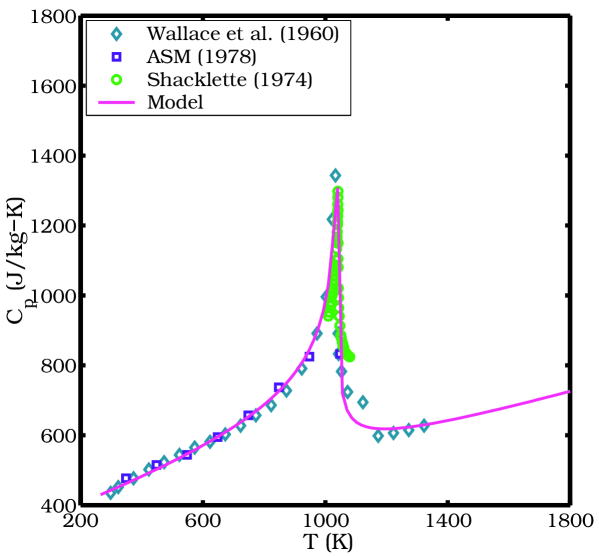
Figure 1: Comparison of experimental data and model prediction of specific heat for 4340 steel as a function of temperature.

Table 1: Constants used in specific heat model for 4340 steel.

$T_{c}$	$A_{1}$	$B_{1}$	$C_{1}$	$\alpha$	$A_{2}$	$B_{2}$	$C_{2}$	$\alpha^{{}^{\prime}}$
(K)	(J/kg-K)	(J/kg-K)	(J/kg-K)		(J/kg-K)	(J/kg-K)	(J/kg-K)
1040	190.14	-273.75	418.30	0.20	465.21	267.52	58.16	0.35

3.2 Melting Temperature Model for 4340 Steel

For the sake of simplicity, we do not consider a phase change in the melting temperature model and assume that the iron crystals remain bcc at all temperatures and pressures. We also assume that iron has the same melting temperature as 4340 steel. In Figure 2 we have plotted experimental data (Burakovsky et al. [8], Williams et al. [45], Yoo et al. [46]) for the melting temperature of iron at various pressures. Melting curves predicted by the SCG model (Equation 13) and the BPS model (Equation 14) are shown as smooth curves on the figure. The BPS model performs better at high pressures, but both models are within experimental error below 100 GPa. We have chosen to use the BPS melting temperature model because of its larger range of applicability.

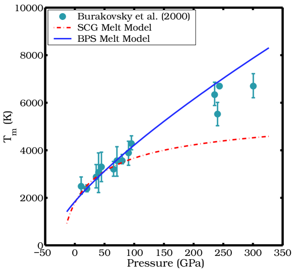
Figure 2: Comparison of experimental data and model predictions of melting temperature for 4340 steel as a function of pressure.

The parameters used for the models are shown in Table 2. An initial density ($\rho_{0}$) of 7830 kg/m³ has been used in the model calculations.

Table 2: Parameters used in melting temperature models for 4340 steel. The SCG model parameters are from Gust [19]. The bulk and shear moduli and their derivatives have been obtained from Guinan and Steinberg [18]. The parameters for the BPS model at zero pressure have been obtained from Burakovsky and Preston [7], Burakovsky et al. [9], and the lattice constant ($a$) is from Jansen et al. [24].

Steinberg-Cochran-Guinan (SCG) model
$T_{m0}(K)$	$\Gamma_{0}$	$a$
1793	1.67	1.67
Burakovsky-Preston-Silbar (BPS) model
$K_{0}$ (GPa)	$K_{0}^{{}^{\prime}}$	$\mu_{0}$ (GPa)	$\mu_{0}^{{}^{\prime}}$	$\kappa$	$z$	$b^{2}\rho_{c}(T_{m})$	$\alpha$	$\lambda$	$v_{WS}$ ($\AA^{3}$)	$a$ ($\AA$)
166	5.29	81.9	1.8	1	8	0.78	2.9	1.30	$a^{3}/2$	2.865

3.3 Shear Modulus Models for 4340 Steel

Figures 3(a), (b), and (c) show shear moduli predicted by the MTS shear modulus model, the SCG shear modulus model, and the NP shear modulus model, respectively. Three values of compression ($\eta$ = 0.9, 1.0, 1.1) are considered for each model. The pressure-dependent melting temperature has been determined using the BPS model in each case. The initial density is taken to be 7830 kg/m³. The model predictions are compared with experimental data for AISI 1010 steel and SAE 304 stainless steel. As the figure shows, both steels behave quite similarly as far as their shear moduli are concerned. We assume that 4340 steel also shows a similar dependence of shear modulus on temperature.

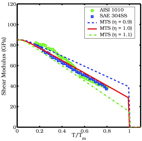
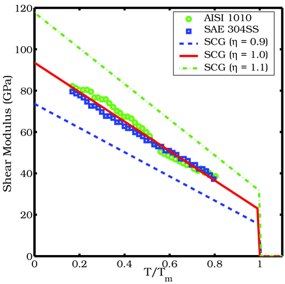
(a) MTS Shear Model                                              (b) SCG Shear Model

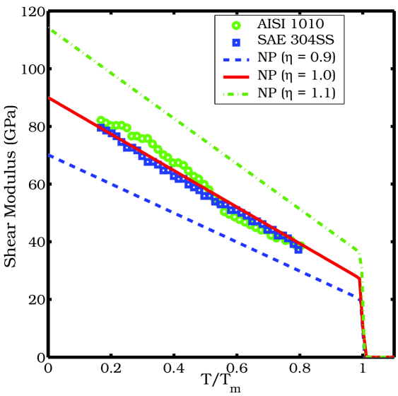
(c) NP Shear Model

Figure 3: Comparison of experimental data with model predictions of shear modulus for 4340 steel. The experimental data are for AISI 1010 steel and SAE 304 stainless steel (Fukuhara and Sanpei [15]) at standard pressure.

The MTS model does not incorporate any pressure dependence of the shear modulus. The pressure dependence observed in Figure 3(a) is due to the pressure dependence of $T_{m}$. Both the SCG and NP shear modulus models are pressure dependent and provide a good fit to the data. Though the SCG model is computationally more efficient than and as accurate as the NP model, we have chosen to the NP shear modulus model for subsequent calculations for 4340 steel because of its smooth transition to zero shear modulus at melt.

The parameters used in the shear modulus models are shown in Table 3. The parameters for the MTS model have been obtained from a least squares fit to the data at a compression of 1. The values of $\mu_{0}$ and $\partial\mu/\partial p$ for the SCG model are from Guinan and Steinberg [18]. The derivative with respect to temperature has been chosen so as to fit the data at a compression of 1. The NP shear model parameters $\mu_{0}$ and $C$ have also been chosen to fit the data. A value of 0.57 for $C$ is suggested by Nadal and Le Poac [35]. However, that value leads to a higher value of $\mu$ at high temperatures than suggested by the experimental data.

Table 3: Parameters used in shear modulus models for 4340 steel.

MTS shear modulus model
$\mu_{0}$ (GPa)	$D$ (GPa)	$T_{0}$ (K)
85.0	10.0	298
SCG shear modulus model
$\mu_{0}$ (GPa)	$\partial\mu/\partial p$	$\partial\mu/\partial T$ (GPa/K)
81.9	1.8	0.0387
NP shear modulus model
$\mu_{0}$ (GPa)	$\partial\mu/\partial p$	$\zeta$	$C$	$m$ (amu)
90.0	1.8	0.04	0.080	55.947

3.4 Equation of State for 4340 Steel

The pressure in the steel is calculated using the Mie-Grüneisen equation of state (equation  20) assuming a linear Hugoniot relation. The Grüneisen gamma ($\Gamma_{0}$) is assumed to be a constant over the regime of interest. The specific heat at constant volume is assumed to be the same as that at constant pressure and is calculated using equation (11).

Figure 4 compares model predictions with experimental data for iron (Bancroft et al. [1], McQueen et al. [34], Barker and Hollenbach [4]), mild steel (Katz et al. [28]), 300 series stainless steels (McQueen et al. [34]), and for AISI 4340 steel (Gust et al. [20]). The high pressure experimental data are not along isotherms and show the temperature increase due to compression. The equation of state provides a reasonable match to the experimental data at compressions below 1.2 which is reasonable for the simulations of interest in this paper. Improved equations of state should be used for overdriven shocks.

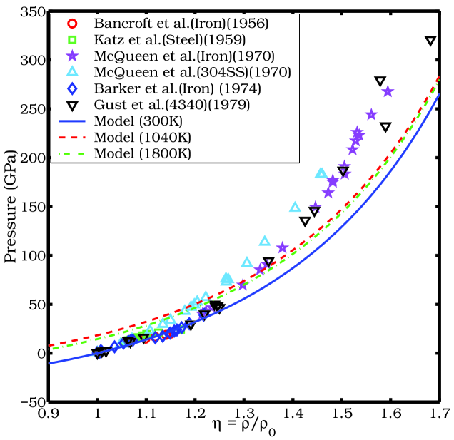
Figure 4: Comparison of experimental data with model predictions of equation of state for 4340 steel.

In the model calculations, the bulk speed of sound ($C_{0}$) is 3935 m/s and the linear Hugoniot slope coefficient ($S_{\alpha}$) is 1.578. Both parameters are for iron and have been obtained from Brown et al. [5]. The Grüneisen gamma value ($\Gamma_{0}$ = 1.69) has been interpolated from values given by Gust et al. [20]. An initial temperature ($T_{0}$) of 300 K and an initial density of 7830 kg/m³ have been used in the model calculations.

4 Determination of MTS Model Parameters

The yield strength of high-strength low-alloy (HSLA) steels such as 4340 steel can vary dramatically depending on the heat treatment that it has undergone. This is due to the presence of bcc ferrite-bainite phases along with the dominant bcc martensite phase at room temperature. At higher temperatures (below the $\alpha$-$\gamma$ transition) the phases partially transform into the fcc austenite and much of the effect of heat treatment is expected to be lost. Beyond the transition temperature, the alloy is mostly the fcc $\gamma$ phase that is expected to behave differently than the lower temperature phases. Hence, purely empirical plasticity models have to be recalibrated for different levels of hardness of 4340 steel and for different ranges of temperature.

In the absence of relevant microstructural models for the various tempers of 4340 steel, we assume that there is a direct correlation between the Rockwell C hardness of the alloy steel and the yield stress (see the ASM Handbook [21]). We determine the MTS parameters for four tempers of 4340 steel. Empirical relationships are then determined that can be used to calculate the parameters of intermediate tempers of 4340 steel via interpolation.

The experimental data used to determine the MTS model parameters are from the sources shown in Table 4. All the data are for materials that have been oil quenched after austenitization. More details can be found in the cited references. The 4340 VAR (vacuum arc remelted) steel has a higher fracture toughness than the standard 4340 steel. However, both steels have similar yield behavior (Brown et al. [6]).

Table 4: Sources of experimental data for 4340 steel.

Material	Hardness	Normalize	Austenitize	Tempering	Reference
		Temp. (C)	Temp. (C)	Temp. (C)
4340 Steel	$R_{c}$ 30				Johnson and Cook [26]
4340 Steel	$R_{c}$ 38	900	870	557	Larson and Nunes [31]
4340 Steel	$R_{c}$ 38		850	550	Lee and Yeh [33]
4340 VAR Steel	$R_{c}$ 45	900	845	425	Chi et al. [12]
4340 VAR Steel	$R_{c}$ 49	900	845	350	Chi et al. [12]

The experimental data are either in the form of true stress versus true strain or shear stress versus average shear strain. These curves were digitized manually with care and corrected for distortion. The error in digitization was around 1% on average. The shear stress-strain curves were converted into an effective tensile stress-strain curves assuming von Mises plasticity (see Goto et al. [16]). The elastic portion of the strain was then subtracted from the total strain to get true stress versus plastic strain curves. The Young’s modulus was assumed to be 213 MPa.

4.1 Determination of $\sigma_{a}$

The first step in the determination of the parameters for the MTS models is the estimation of the athermal component of the yield stress ($\sigma_{a}$). This parameter is dependent on the Hall-Petch effect and hence on the characteristic martensitic packet size. The packet size will vary for various tempers of steel and will depend on the size of the austenite crystals after the $\alpha$-$\gamma$ phase transition. Since we do not have unambiguous grain sizes and other information needed to determine $\sigma_{a}$, we assume that this constant is independent of temper and has a value of 50 MPa based on the value used for HY-100 steel (Goto et al. [16]). We have observed that a value of 150 MPa leads to a better fit to the modified Arrhenius equation for $\sigma_{i}$ and $g_{0i}$ for the $R_{c}$ 30 temper. However, this value is quite high and probably unphysical because of the relatively large grain size at this temper.

4.2 Determination of $\sigma_{i}$ and $g_{0i}$

From equation (1), it can be seen that $\sigma_{i}$ can be found if $\sigma_{y}$ and $\sigma_{a}$ are known and $\sigma_{e}$ is zero. Assuming that $\sigma_{e}$ is zero when the plastic strain is zero, and using equation (2), we get the relation

$$\left(\cfrac{\sigma_{y}-\sigma_{a}}{\mu}\right)^{p_{i}}=\left(\cfrac{\sigma_{i}}{\mu_{0}}\right)^{p_{i}}\left[1-\left(\cfrac{1}{g_{0i}}\right)^{1/q_{i}}\left[\cfrac{k_{b}T}{\mu b^{3}}\ln\left(\cfrac{\dot{\epsilon}_{0i}}{\dot{\epsilon}}\right)\right]^{1/q_{i}}\right]$$ (22)

Modified Arrhenius (Fisher) plots based on equation (22) are used to determine the normalized activation energy ($g_{0i}$) and the intrinsic thermally activated portion of the yield stress ($\sigma_{i}$). The parameters $p_{i}$ and $q_{i}$ for iron and steels (based on the effect of carbon solute atoms on thermally activated dislocation motion) have been suggested to be 0.5 and 1.5, respectively (Kocks et al. [30], Goto et al. [16]). Alternative values can be obtained depending on the assumed shape of the activation energy profile or the obstacle force-distance profile (Cottrell and Bilby [13], Caillard and Martin [10]).

We have observed that the values suggested for HY-100 give us a value of the normalized activation energy $g_{0i}$ for $R_{c}$ = 30 that is around 40, which is not physical. Instead, we have assumed a rectangular force-distance profile which gives us values of $p_{i}$ = 2/3 and $q_{i}=1$ and reasonable values of $g_{0i}$. We have assumed that the reference strain rate is $\dot{\epsilon}_{0i}=10^{8}$/s.

The Fisher plots of the raw data (based on Equation (22)) are shown as squares in Figures 5(a), (b), (c), and (d). Straight line least squares fits to the data are also shown in the figures. For these plots, the shear modulus ($\mu$) has been calculated using the NP shear modulus model discussed in Sections 2.4.3 and 3.3. The yield stress at zero plastic strain ($\sigma_{y}$) is the intersection of the stress-plastic strain curve with the stress axis. The value of the Boltzmann constant ($k_{b}$) is 1.3806503e-23 J/K and the magnitude of the Burgers’ vector ($b$) is assumed to be 2.48e-10 m. The density of the material is assumed to be constant with a value of 7830 kg/m³. The raw data used in these plots are given in Appendix A.

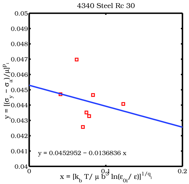
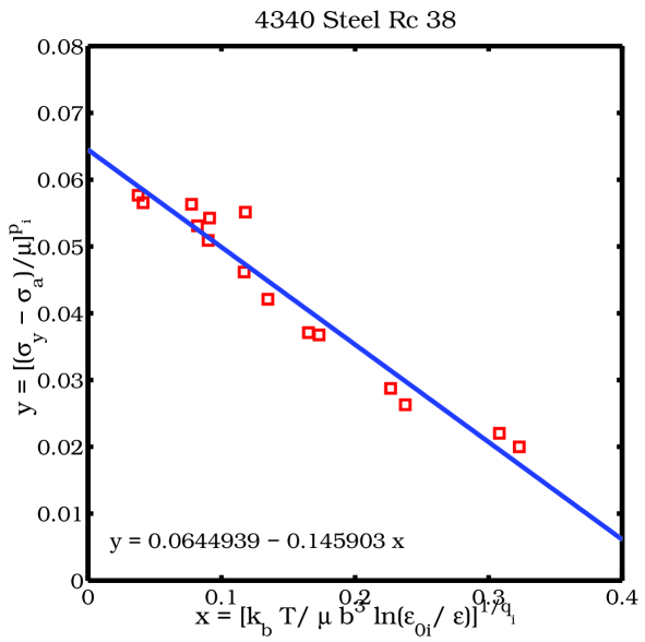
(a) $R_{c}$ = 30                                              (b) $R_{c}$ = 38

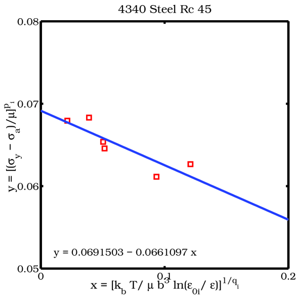
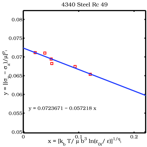
(c) $R_{c}$ = 45                                              (d) $R_{c}$ = 49

Figure 5: Fisher plots for the intrinsic component of the MTS model for various tempers of 4340 steel.

The spread in the data for $R_{c}$ 30 (Figure 5(a)) is quite large and a very low $R^{2}$ value is obtained for the fit. This error is partially due to the inclusion of both tension and shear test data (in the form of effective tensile stress) in the plot. Note that significantly different yield stresses can be obtained from tension and shear tests (especially at large strains) (Johnson and Cook [26], Goto et al. [16]). However, this difference is small at low strains and is not expected to affect the intrinsic part of the yield stress much. A more probable cause of the spread is that the range of temperatures and strain rates is quite limited. More data at higher strain rates and temperatures are needed to get an improved correlation for the $R_{c}$ 30 temper of 4340 steel.

Figure 5(b) shows the fit to the Fisher plot data for 4340 steel of hardness $R_{c}$ 38. The low strain rate data from Larson and Nunes [31] are the outliers near the top of the plot. The hardness of this steel was estimated from tables given in  [21] based on the heat treatment and could be higher than $R_{c}$ 38. However, the Larson and Nunes [31] data are close to the data from Lee and Yeh [33] as can be seen from the plot. A close examination of the high temperature data shows that there is a slight effect due to the $\alpha$ to $\gamma$ phase transformation at high temperatures.

The stress-strain data for 4340 steel $R_{c}$ 45 shows anomalous temperature dependent behavior under quasistatic conditions. For instance, the yield stress at 373 K is higher than that at 298 K. The fit to the Fisher plot data for this temper of steel is shown in Figure 5(c). The fit to the data can be improved if the value of $\sigma_{a}$ is assumed to be 150 MPa and $q_{i}$ is assumed to be equal to 2. However, larger values of $\sigma_{a}$ can lead to large negative values of $\sigma_{e}$ at small strains - which is unphysical.

The fit to the Fisher data for the $R_{c}$ 49 temper is shown in Figure 5(d). The fit is reasonably good. More data at high strain rates and high temperatures are needed for both the $R_{c}$ 45 and the $R_{c}$ 49 tempers of 4340 steel.

The values of $\sigma_{i}$ and $g_{0i}$ for the four tempers of 4340 are shown in Table 5. The value of $g_{0i}$ for the $R_{c}$ 38 temper is quite low and leads to values of the Arrhenius factor ($S_{i}$) that are zero for temperatures more than 800 K. In the following section, we consider the effect of dividing the $R_{c}$ 38 data into high and low temperature regions to alleviate this problem.

Table 5: Values of $\sigma_{i}$ and $g_{0i}$ for four tempers of 4340 steel.

Hardness ($R_{c}$)	$\sigma_{i}$ (MPa)	$g_{0i}$
30	867.6	3.31
38	1474.1	0.44
45	1636.6	1.05
49	1752	1.26

4.2.1 High temperature values of $\sigma_{i}$ and $g_{0i}$

More data at higher temperatures and high strain rates are required for better characterization of the $R_{c}$ 30, $R_{c}$ 45, and $R_{c}$ 49 tempers of 4340 steel. In the absence of high temperature data, we can use data for the $R_{c}$ 38 temper at high temperatures to obtain the estimates of $\sigma_{i}$ and $g_{0i}$ for other tempers. We explore two approaches of determining these parameters:

1. Case 1: Divide the temperature regime into three parts: $T_{0}<$ 573 K; 573 K $\leq T_{0}<$ 1040 K; $T_{0}\geq$ 1040 K. The values of $\sigma_{i}$ and $g_{0i}$ are calculated for each of these regimes from the $R_{c}$ 38 data. The values of the two parameters for temperatures above 573 K are assumed to be applicable to all the tempers. Note that the choice of 573 K for the cut-off temperature is arbitrary and loss of temper is likely to occur at a higher temperature.

2. Case 2: Divide the temperature regime into two parts: $T_{0}<$ 1040 K and $T_{0}\geq$ 1040 K. In this case, we assume that the various tempers retain distinctive properties up to the phase transition temperature. All the tempers are assumed to have identical values of $\sigma_{i}$ and $g_{0i}$ above 1040 K.

Case 1: Three temperature regimes.

The low and high temperature Fisher plots for $R_{c}$ 38 4340 steel are shown in Figures 6 (a) and (b), respectively.

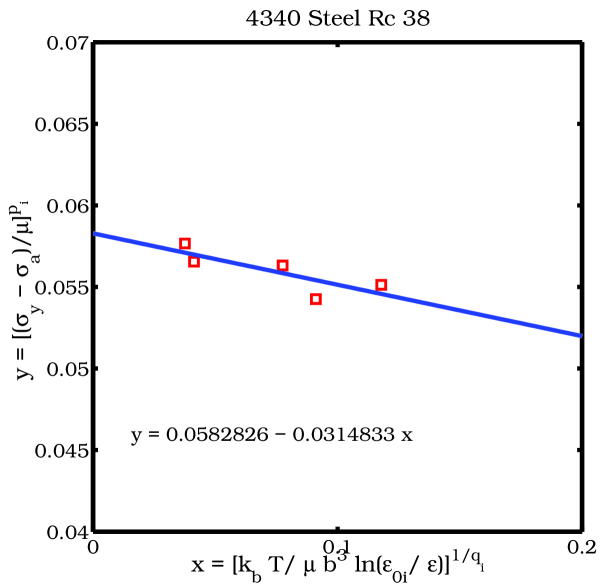
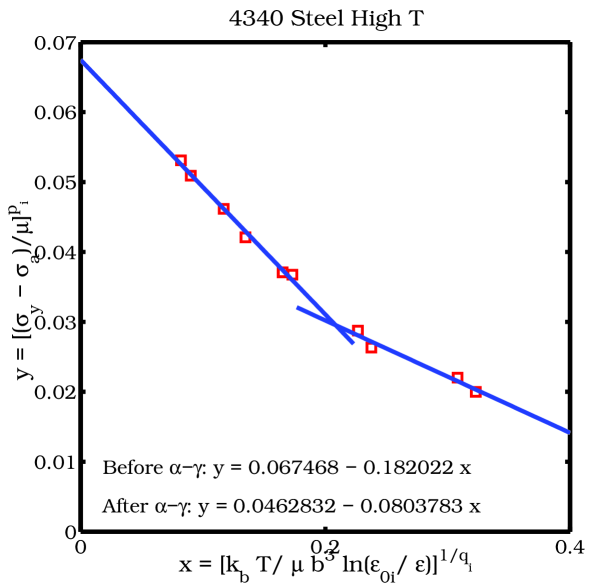
(a) $R_{c}$ = 38 (T $<$ 573 K)                        (b) $R_{c}$ = 38 (T $>$ 573 K)

Figure 6: Fisher plots for the intrinsic component of the MTS model for $R_{c}$ 38 4340 steel assuming three temperature regimes.

A comparison of Figures 5(b) and 6(a) shows that the low temperature Fisher plot has a distinctly lower slope that the plot that contains all the $R_{c}$ 38 data. The values of $\sigma_{i}$ and $g_{0i}$ at low temperatures for the $R_{c}$ 38 temper are 1266 MPa and 1.85, respectively. The high temperature plot (Figure 6(b)) shows that the slope of the Fisher plot is quite steep between 573 K and 1040 K and decreases slightly after the $\alpha$ to $\gamma$ phase transition. The values of $\sigma_{i}$ and $g_{0i}$ for temperatures between 573 K and 1040 K are 1577.2 MPa and 0.371, respectively. After the phase transition at 1040 K, these quantities take values of 896.1 MPa and 0.576, respectively.

Plots of $\sigma_{i}$ and $g_{0i}$ as functions of the Rockwell hardness number (for temperatures below 573 K) are shown in Figures 7(a) and (b), respectively. These plots show a smooth increase in the value of $\sigma_{i}$ and a decrease in the normalized activation energy ($g_{0i}$) with increasing hardness.

(a) $\sigma_{i}$                                              (b) $g_{0i}$

Figure 7: Values of $\sigma_{i}$ and $g_{0i}$ obtained from the Fisher plots for various tempers of 4340 steel close to room temperature (for the three temperature regime).

The high temperature values of $g_{0i}$ for the $R_{c}$ 38 give reasonable values of $S_{i}$ (non-zero) at temperatures above 800 K. However, the lower temperature (less that 1040 K) values of the two parameters give a poor fit to the experimental stress-strain data. This is probably due to the anomalous behavior of 4340 steel at 373 K and low strain rates.

Case 2: Two temperature regimes.

The two-regime fits to the Fisher plot data for $R_{c}$ 38 are shown in Figure 8.

Figure 8: Fisher plots for the intrinsic component of the MTS model for the $\alpha$ and $\gamma$ phases of $R_{c}$ 38 4340 steel assuming two temperature regimes.

The values of $\sigma_{i}$ and $g_{0i}$ for the $R_{c}$ 38 temper (in the $\alpha$ phase) are 1528 MPa and 0.412, respectively, while those for the $\gamma$ phase are 896 MPa and 0.576, respectively. The fits show a jump in value at 1040 K that is not ideal for Newton iterations in a typical elastic-plastic numerical code. We suggest that the $\gamma$ phase values of these parameters be used if there is any problem with convergence.

Plots of $\sigma_{i}$ and $g_{0i}$ as functions of the Rockwell hardness number (for temperatures below 1040 K) are shown in Figures 9(a) and (b), respectively. Straight line fits to the $\sigma_{i}$ and $g_{0i}$ versus $R_{c}$ data can be used to estimate these parameters for intermediate tempers of the $\alpha$ phase of 4340 steel. These fits are shown in Figure 9.

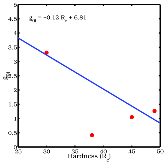
(a) $\sigma_{i}=44.628R_{c}-361.33$             (b) $g_{0i}=-0.1195R_{c}+6.814$

Figure 9: Values of $\sigma_{i}$ and $g_{0i}$ obtained from the Fisher plots for various tempers of the $\alpha$ phase of 4340 steel. The fit for $g_{0i}$ excludes the low value for $R_{c}$ 38 4340 steel.

The value of $\sigma_{i}$ increases with increasing hardness. However, the value of $g_{0i}$ does not decrease monotonically with hardness. More experimental data are needed to determine if the trend of $g_{0i}$ is physical. The value of $g_{0i}$ for the $R_{c}$ 38 temper appears to be unusually low. However, these values lead to good fit to experimental data for $R_{c}$ 38 temper. For that reason, we have used the two temperature regime values of $\sigma_{i}$ and $g_{0i}$ for all subsequent computations that use these parameters.

4.3 Determination of $\sigma_{0es}$ and $g_{0es}$

Once estimates have been obtained for $\sigma_{i}$ and $g_{0i}$, the value of $S_{i}\sigma_{i}$ can be calculated for a particular strain rate and temperature. From equation (1), we then get

$$\sigma_{e}=\cfrac{1}{S_{e}}\left[\cfrac{\mu_{0}}{\mu}\left(\sigma_{y}-\sigma_{a}\right)-S_{i}\sigma_{i}\right]~{}.$$ (23)

Equation (23) can be used to determine the saturation value ($\sigma_{es}$) of the structural evolution stress ($\sigma_{e}$). Given a value of $\sigma_{es}$, equation (9) can be used to compute $\sigma_{0es}$ and the corresponding normalized activation energy ($g_{0es}$) from the relation

$$\ln(\sigma_{es})=\ln(\sigma_{0es})-\frac{k_{b}T}{g_{0es}b^{3}\mu}\ln\left(\cfrac{\dot{\epsilon}}{\dot{\epsilon}_{0es}}\right)~{}.$$ (24)

The value of $\sigma_{es}$ can be determined either from a plot of $\sigma_{e}$ versus the plastic strain or from a plot of the tangent modulus $\theta(\sigma_{e})$ versus $\sigma_{e}$. The value of $S_{e}$ is required before $\sigma_{e}$ can be calculated. Following Goto et al. [16], we assume that $\dot{\epsilon}_{0e}$, $\dot{\epsilon}_{0es}$, $p_{e}$, $q_{e}$, and $g_{0e}$ take the values 10⁷ /s, 10⁷ /s, 2/3, 1, and 1.6, respectively. These values are used to calculate $S_{e}$ at various temperatures and strain rates. The values of $\sigma_{i}$ and $g_{0i}$ used to compute $\sigma_{e}$ vary with hardness for temperatures below 1040 K, and are constant above that temperature as discussed in the previous section. Adiabatic heating is assumed for strain rates greater than 500 /s.

Representative plots of $\sigma_{e}$ versus the plastic strain are shown in Figure 10(a) and the corresponding $\theta$ versus $\sigma_{e}$ plots are shown in Figure 10(b) (for the $R_{c}$ 38 temper; strain rate of 1500 /s). Similar plots for the $R_{c}$ 49 temper for a strain rate of 0.0001 /s are shown in Figures 10(c) and (d). The plotted value of the tangent modulus ($\theta$) is the mean of the tangent moduli at each value of $\sigma_{e}$ (except for the end points where a single value is used). The saturation stress ($\sigma_{es}$) is the value at which $\sigma_{e}$ becomes constant or $\theta$ is zero. Note that errors in the fitting of $\sigma_{i}$ and $g_{0i}$ can cause the computed value of $\sigma_{e}$ to nonzero at zero plastic strain.

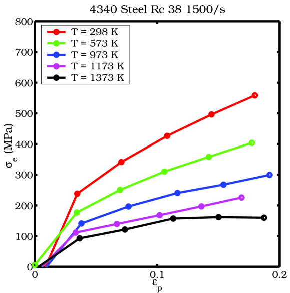
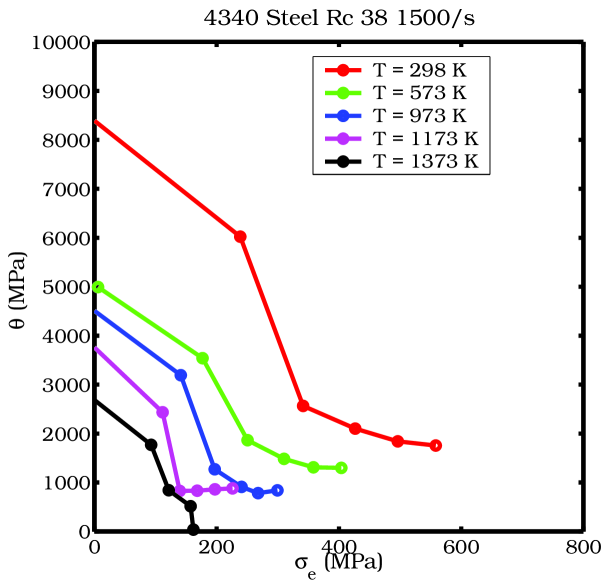
(a) $\sigma_{e}$ vs. $\epsilon_{p}$ ($R_{c}$ 38 1500 /s)                        (b) $\theta$ vs. $\sigma_{e}$ ($R_{c}$ 38 1500 /s)

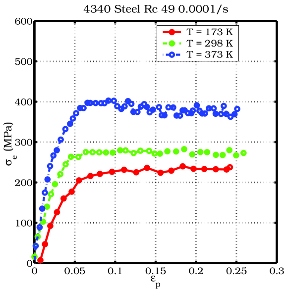
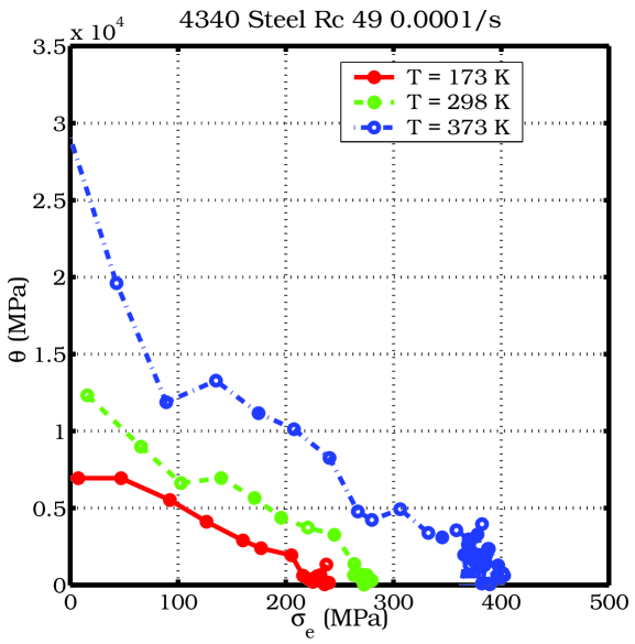
(c) $\sigma_{e}$ vs. $\epsilon_{p}$ ($R_{c}$ 49 0.0001 /s)                        (d) $\theta$ vs. $\sigma_{e}$ ($R_{c}$ 49 0.0001 /s)

Figure 10: Plots used to determine the saturation value ($\sigma_{es}$) of the structure evolution stress ($\sigma_{e}$).

The raw data used to plot the Fisher plots for $\sigma_{0es}$ and $g_{0es}$ are given in Appendix B. These data are plotted in Figures 11(a), (b), (c), and (d). The straight line fit to the data for the $R_{c}$ 30 temper is shown in Figure 11(a). The fit to the $\alpha$ phase for $R_{c}$ 38 4340 steel is shown in Figure 11(b). Similar Fisher plots for $R_{c}$ 45 and $R_{c}$ 49 4340 steel are shown in Figures 11(c) and (d).

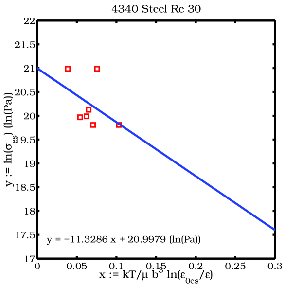
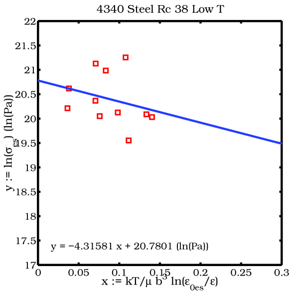
(a) $R_{c}$ = 30                                              (b) $R_{c}$ = 38

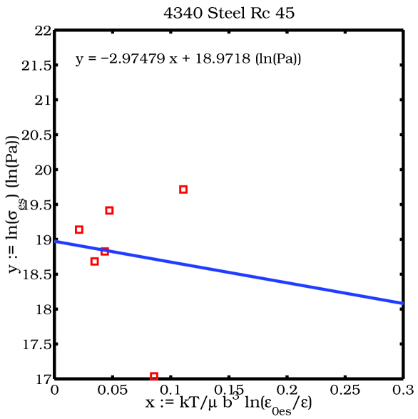
(c) $R_{c}$ = 45                                              (d) $R_{c}$ = 49

Figure 11: Fisher plots for the structure evolution dependent component of the MTS model for the $\alpha$ phase of various tempers of 4340 steel.

The correlation between the modified Arrhenius relation and the data is quite poor. Considering the fact that special care has been taken to determine the value of $\sigma_{es}$, the poor fit appears to suggest that the strain dependent part of the mechanical threshold stress does not follow an Arrhenius relation. However, we do not have information on the error in the experimental data and therefore cannot be confident about such a conclusion. We continue to assume, following  [16] for HY-100, that a modified Arrhenius type of temperature and strain rate dependence is acceptable for the strain dependent part of the yield stress of 4340 steel.

Values of $\sigma_{0es}$ and $g_{0es}$ computed from the Fisher plots are shown in Table 6. The value of the saturation stress decreases with increasing hardness while the normalized activation energy (at 0 K) increases with increasing hardness. For intermediate tempers a median value of 0.284 is assumed for $g_{0es}$ and the mean value of 705.5 MPa is assumed for $\sigma_{0es}$. Straight line fits to the data, as shown in Figures 12(a) and (b), could also be used to determine the values of $g_{0es}$ and $\sigma_{0es}$ for intermediate tempers of 4340 steel.

Fits to the data for temperatures greater than 1040 K give us values of $\sigma_{0es}$ and $g_{0es}$ for the $\gamma$ phase of 4340 steel. The values of these parameters at such high temperatures are $g_{0es}=$ 0.294 and $\sigma_{0es}=$ 478.36 MPa.

Table 6: Values of $\sigma_{0es}$ and $g_{0es}$ for four tempers of 4340 steel.

Hardness ($R_{c}$)	$\sigma_{0es}$ (MPa)	$g_{0es}$
30	1316.1	0.088
38	1058.4	0.232
45	173.5	0.336
49	274.9	1.245

(a) $\sigma_{0es}=-63.9R_{c}+3293.4$ (MPa)             (b) $g_{0i}=0.01656R_{c}-0.405$

Figure 12: Values of $\sigma_{0es}$ and $g_{0es}$ obtained from the Fisher plots for various tempers of the $\alpha$ phase of 4340 steel. The dashed lines show the median values of the parameters.

4.4 Determination of hardening rate $\theta$

The modified Voce rule for the hardening rate ($\theta$) (equation (5)) is purely empirical. To determine the temperature and strain rate dependence of $\theta$, we plot the variation of $\theta$ versus the normalized structure evolution stress assuming hyperbolic tangent dependence of the rate of hardening on the mechanical threshold stress. We assume that $\alpha=3$.

Figures 13(a), (b), (c), and (d) show some representative plots of the variation of $\theta$ with $F:=\tanh(\alpha\sigma_{e}/\sigma_{es})/\tanh(\alpha)$.

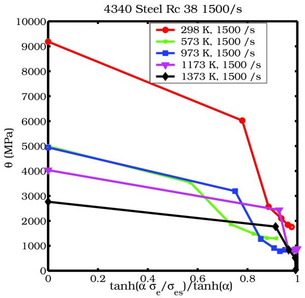
(a) $R_{c}$ 30, Tension                        (b) $R_{c}$ 38, 1500/s

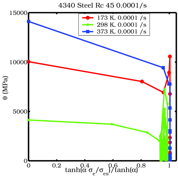
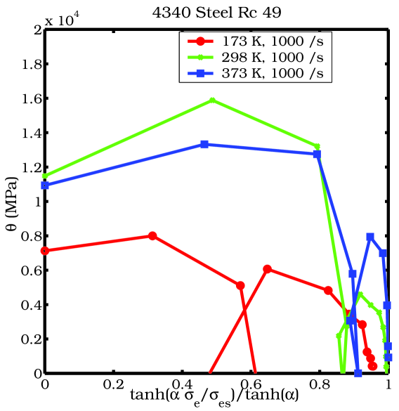
(c) $R_{c}$ 45, 0.0001/s                        (d) $R_{c}$ 49, 1000/s

Figure 13: Plots used to determine $\theta_{0}$ as a function of temperature and strain rate. $\alpha$ = 3.

As the plots show, the value of $\theta_{1}$ (the value of $\theta$ at $F=1$) can be assumed to be zero for most of the data.

It is observed from Figure 13(a) that there is a strong strain rate dependence of $\theta$ that appears to override the expected decrease with increase in temperature for the $R_{c}$ 30 temper of 4340 steel. It can also been seen that $\theta$ is almost constant at 298 K and 0.002/s strain rate reflecting linear hardening. However, the hyperbolic tangent rule appears to be a good approximation at higher temperatures and strain rates.

The plot for $R_{c}$ 38 4340 steel (Figure 13(b)) shows a strong temperature dependence of $\theta$ with the hardening rate decreasing with increasing temperature. The same behavior is observed for all high strain rate data. However, for the data at a strain rate of 0.0002/s, there is an increase in $\theta$ with increasing temperature. Figures 13(c) and (d) also show an increase in $\theta$ with temperature. These reflect an anomaly in the constitutive behavior of 4340 steel for relatively low temperatures (below 400 K) (Tanimura and Duffy [41]) that cannot be modeled continuously using an Arrhenius law and needs to be characterized in more detail.

Fits to the experimental data of the form shown in equation (6) have been attempted. The resulting values of $a_{00}$, $a_{01}$, $a_{02}$, and $a_{03}$ are plotted as functions of $R_{c}$ in Figures 14(a), (b), (c), and (d), respectively. The points show the values of the constants for individual tempers while the solid line shows the median value.

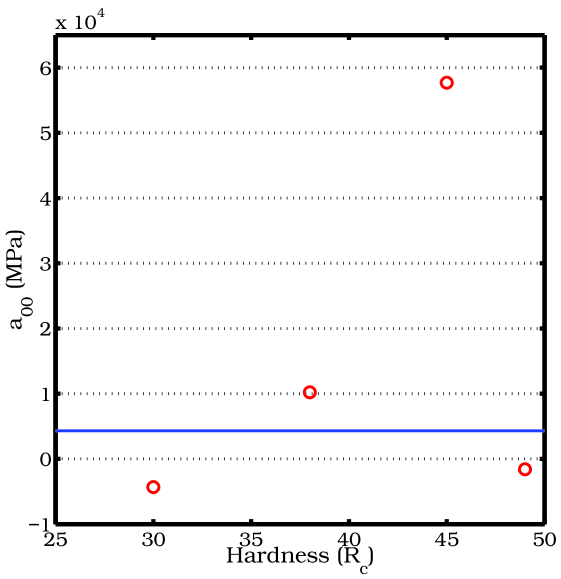
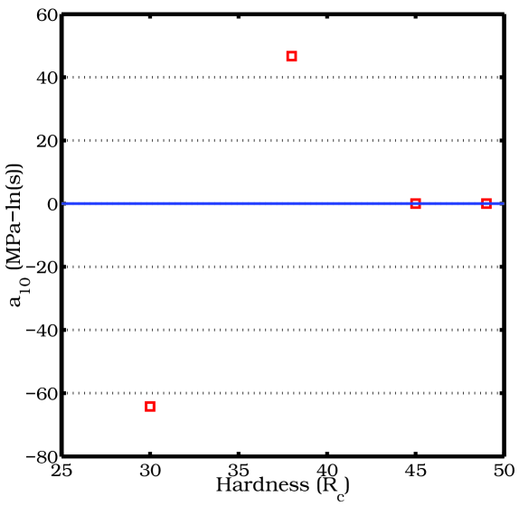
(a) $a_{00}$ vs. $R_{c}$                        (b) $a_{10}$ vs. $R_{c}$

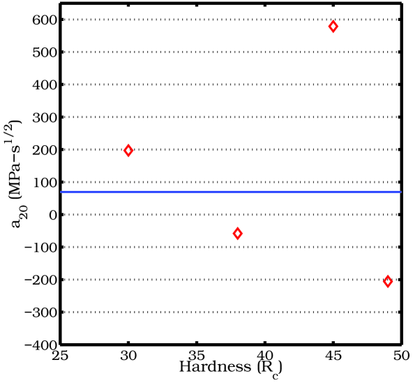
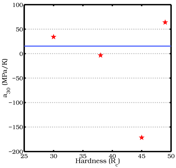
(c) $a_{20}$ vs. $R_{c}$                        (d) $a_{30}$ vs. $R_{c}$

Figure 14: Variation of the constants fit to the hardening rate equation for various tempers of 4340 steel.

These figures show that the constants vary considerably and also change sign for different tempers. On average, the strain rate dependence is small for all the tempers but significant. The $R_{c}$ 30 and $R_{c}$ 45 data points in Figure 14(d) reflect an increase in hardening rate with temperature that is nonphysical at high temperatures.

Instead of using these fits to the experimental data, we have decided to ignore the strain rate dependence of the hardening rate and fit a curve to all the data taking only temperature dependence into account (as shown in Figure 15). Distinctions have not been made between various tempers of 4340 steel to determine this average hardening rate. However, we do divide the data into two parts based on the $\alpha$-$\gamma$ phase transition temperature.

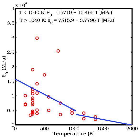
Figure 15: Variation of $\theta_{0}$ with temperature.

The resulting equations for $\theta_{0}$ as functions of temperature are

$$\theta_{0}=\begin{cases}15719-10.495~{}T~{}\text{(MPa)}&\text{for}~{}T<1040K\\ 7516-3.7796~{}T~{}\text{(MPa)}&\text{for}~{}T>1040K\end{cases}$$ (25)

This completes the determination of the parameters for the MTS model.

5 Comparison of MTS model predictions and experimental data

The performance of the MTS model for 4340 steel is compared to experimental data in this section. In the figures that follow, the MTS predictions are shown as dotted lines while the experimental data are shown as solid lines with symbols indicting the conditions of the test. Isothermal conditions have been assumed for strain rates less than 500/s and adiabatic heating is assumed to occurs at higher strain rates.

Figure 16(a) shows the low strain rate experimental data and the corresponding MTS predictions for the $R_{c}$ 30 temper of 4340 steel. Comparisons for moderately high strain rates and high temperatures for the $R_{c}$ 30 temper are shown in Figure 16(b). The model matches the experimental curves quite well for low strain rates (keeping in mind the difference between the stress-strain curves in tension and in shear). The high strain rate curves are also accurately reproduced though there is some error in the initial hardening modulus for the 650 /s and 735 K case. This error can be eliminated if the effect of strain rate is included in the expression for $\theta_{0}$. The maximum modeling error for this temper varies between 5% to 10%.

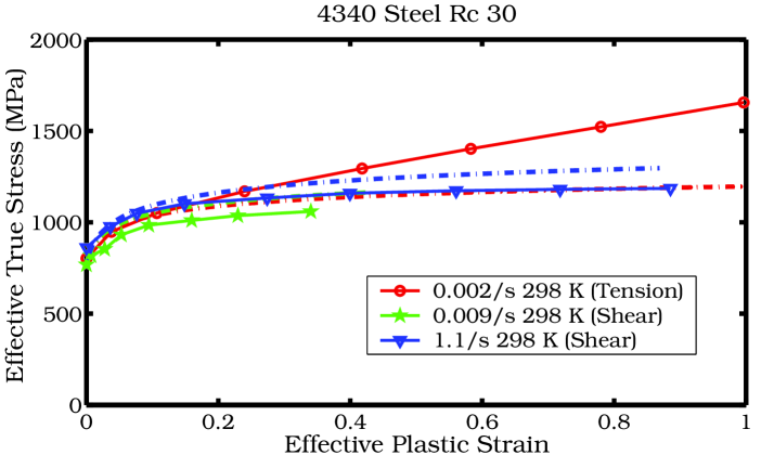
(a) Low strain rates.

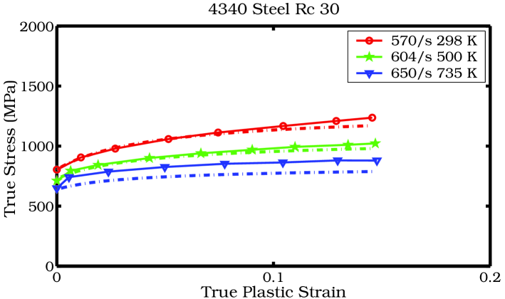
(b) High strain rates.

Figure 16: Comparison of MTS prediction with experimental data from Johnson and Cook [26] for the $R_{c}$ 30 temper of 4340 steel.

We have not used the $R_{c}$ 32 experimental data to fit the MTS model parameters. As a check of the appropriateness of the relation between the parameters and the $R_{c}$ hardness number, we have plotted the MTS predictions versus the experimental data for this temper in Figure 17. Our model predicts a stronger temperature dependence for this temper than the experimental data. However, the initial high temperature yield stress is reproduced quite accurately while the ultimate tensile stress is reproduced well for the lower temperatures.

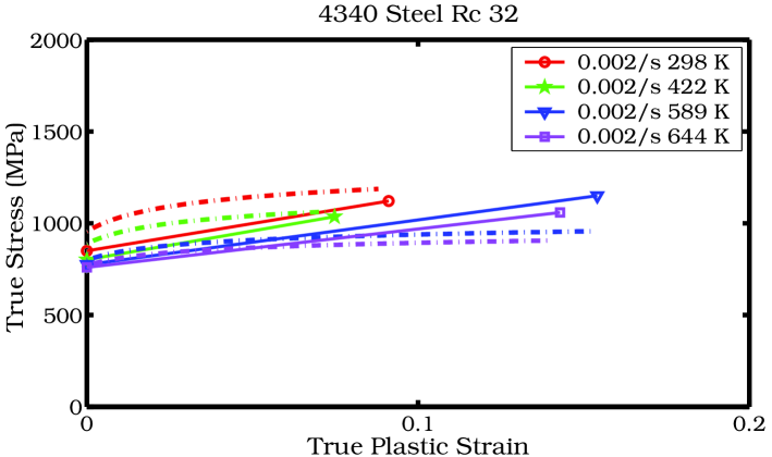
Figure 17: Comparison of MTS prediction with experimental data from Brown et al. [6] for the $R_{c}$ 32 temper of 4340 steel.

The low strain rate stress-strain curves for $R_{c}$ 38 4340 steel are shown in Figure 18. High strain rate stress-strain curves for the $R_{c}$ 38 temper are shown in Figures 19(a), (b), and (c). The saturation stress predicted at low strain rates is around 20% smaller than the observed values at large strains. The anomaly at 373 K is not modeled accurately by the MTS parameters used. On the other hand, the high strain rate data are reproduced quite accurately by the MTS model with a modeling error of around 5% for all temperatures.

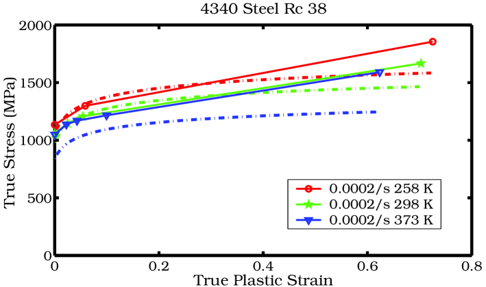
Figure 18: Comparison of MTS prediction with experimental data from Larson and Nunes [31] for the $R_{c}$ 38 temper of 4340 steel at 0.0002/s strain rate.

(a) Strain Rate = 500 /s

(b) Strain Rate = 1500 /s

(c) Strain Rate = 2500 /s

Figure 19: Comparison of MTS prediction with experimental data from Lee and Yeh [33] for the $R_{c}$ 38 temper of 4340 steel at high strain rates.

Experimental data for the $R_{c}$ 45 temper are compared with MTS predictions in Figures 20 (a) and (b). The MTS model underpredicts the low strain rate yield stress and initial hardening modulus by around 15% for both the 173 K and 373 K data. The prediction is within 10% for the 298 K data. The anomaly at 373 K is clearly visible for the low strain rate plots shown in Figure 20(a). The high strain rate data are reproduced quite accurately for all three temperatures and the error is less than 10%.

(a) Strain Rate = 0.0001 /s

(b) Strain Rate = 1000 /s

Figure 20: Comparison of MTS prediction with experimental data from Chi et al. [12] for the $R_{c}$ 45 temper of 4340 steel.

Comparisons for the $R_{c}$ 49 temper are shown in Figures 21 (a) and (b). The model predicts the experimental data quite accurately for 173 K and 298 K at a strain rate of 0.0001/s. However, the anomalous behavior at 373K is not predicted and a modeling error of around 15% is observed for this temperature. For the high strain rate cases shown in Figure 21(b), the initial hardening modulus is under-predicted and saturation is predicted at a lower stress than observed. In this case, the modeling error is around 10%.

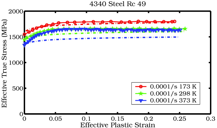
(a) Strain Rate = 0.0001 /s

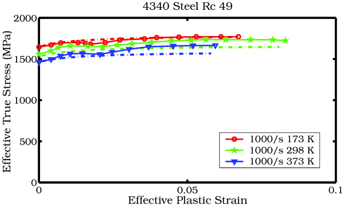
(b) Strain Rate = 1000 /s

Figure 21: Comparison of MTS prediction with experimental data from Chi et al. [12] for the $R_{c}$ 49 temper of 4340 steel.

The comparisons of the MTS model predictions with experimental data shows that the predictions are all within an error of 20% for the range of data examined. If we assume that the standard deviation of the experimental data is around 5% (Hanson [22]) then the maximum modeling error is around 15% with around a 5% mean. This error is quite acceptable for numerical simulations, provided the simulations are conducted within the range of conditions used to fit the data.

6 MTS model predictions over an extended range of conditions

In this section, we compare the yield stresses predicted for a $R_{c}$ 40 temper of 4340 steel by the MTS model with those predicted by the Johnson-Cook (JC) model. A large range of strain rates and temperatures is explored. In the plots shown below, the yield stress ($\sigma_{y}$) is the Cauchy stress, the plastic strain ($\epsilon_{p}$) is the true plastic strain, the temperatures ($T$) are the initial temperatures and the strain rates $\dot{\epsilon}$ are the nominal strain rates. The effect of pressure on the density and melting temperature has been ignored in the MTS calculations presented in this section. The Johnson-Cook model and relevant parameters are discussed in Appendix C.

6.1 Yield stress versus plastic strain

Figures 22(a) and (b) show the yield stress-plastic strain curves predicted by the MTS and JC models, respectively. The initial temperature is 600 K and adiabatic heating is assumed for strain rates above 500 /s. The strain rate dependence of the yield stress is less pronounced for the MTS model than for the JC model. The hardening rate is higher at low strain rates for the JC model. The expected rapid increase in the yield stress at strain rates above 1000 /s (Nicholas [36]) is not predicted by either model. This error is probably due to the limited high rate data used to determine the MTS model parameters.

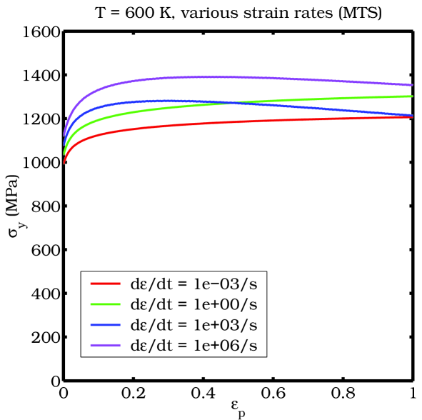
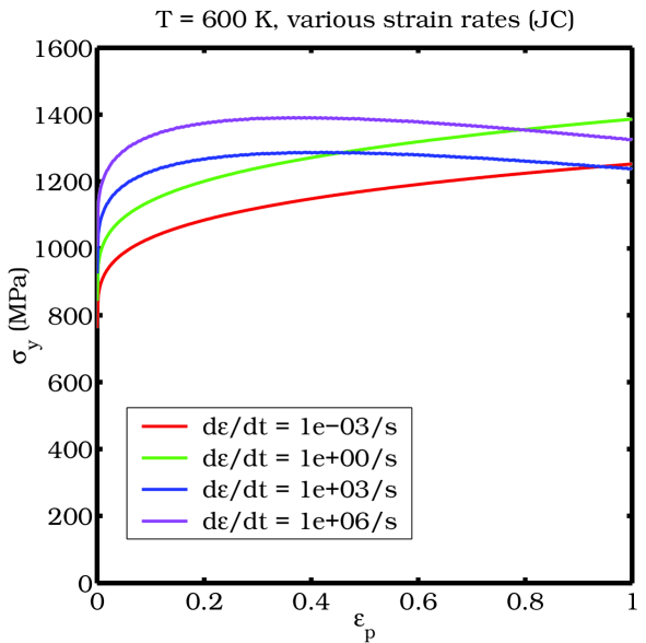
(a) MTS Prediction.                        (b) JC Prediction.

Figure 22: Comparison of MTS and JC predictions of yield stress versus plastic strain at various strain rates for $T_{0}$ = 600 K.

The temperature dependence of the yield stress for a strain rate of 1000 /s is shown in Figures 23(a) and (b). Both models predict similar stress-strain responses as a function of temperature. However, the initial yield stress is higher for the MTS model and the initial hardening rate is lower that that predicted by the JC model for initial temperatures of 300K and 700 K. For the high temperature data, the MTS model predicts lower yield stresses.

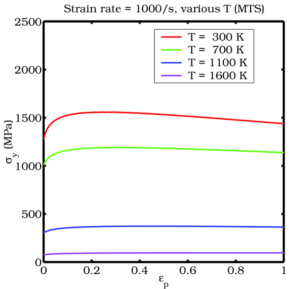
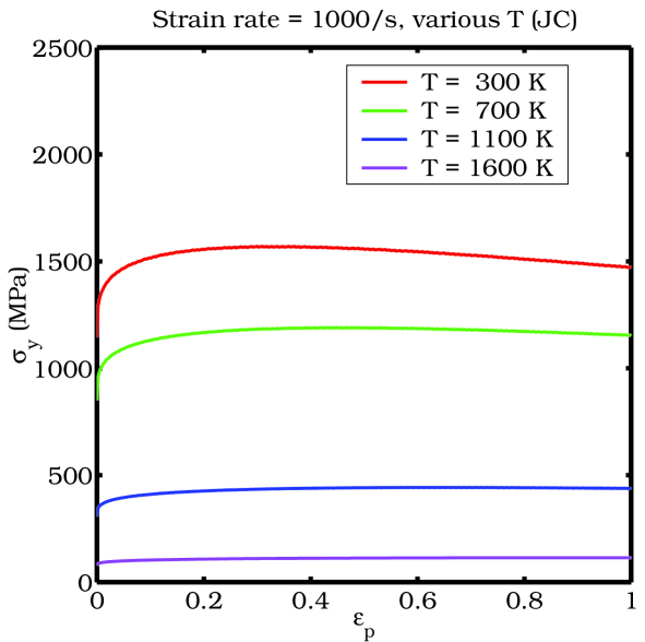
(a) MTS Prediction.                        (b) JC Prediction.

Figure 23: Comparison of MTS and JC predictions of yield stress versus plastic strain at various strain rates for $\dot{\epsilon}$ = 1000 /s.

6.2 Yield stress versus strain rate

The strain rate dependence of the yield stress (at a temperature of 600 K) predicted by the MTS and JC models is shown in Figures 24(a) and (b), respectively. The JC model shows a higher amount of strain hardening than the MTS model. The strain rate hardening of the MTS model appears to be closer to experimental observations (Nicholas [36]) than the JC model.

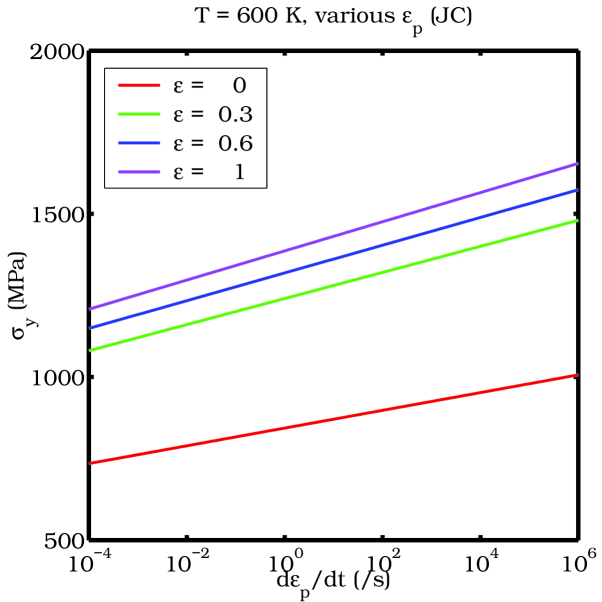
(a) MTS Prediction.                        (b) JC Prediction.

Figure 24: Comparison of MTS and JC predictions of yield stress versus strain rate at various plastic strains for $T_{0}$ = 600 K.

The temperature and strain rate dependence of the yield stress at a plastic strain of 0.3 is shown in Figures 25(a) and (b). Above the phase transition temperature, the MTS model predicts more strain rate hardening than the JC model. However, at 700 K, both models predict quite similar yield stresses. At room temperature, the JC model predicts a higher rate of strain rate hardening than the MTS model and is qualitatively closer to experimental observations.

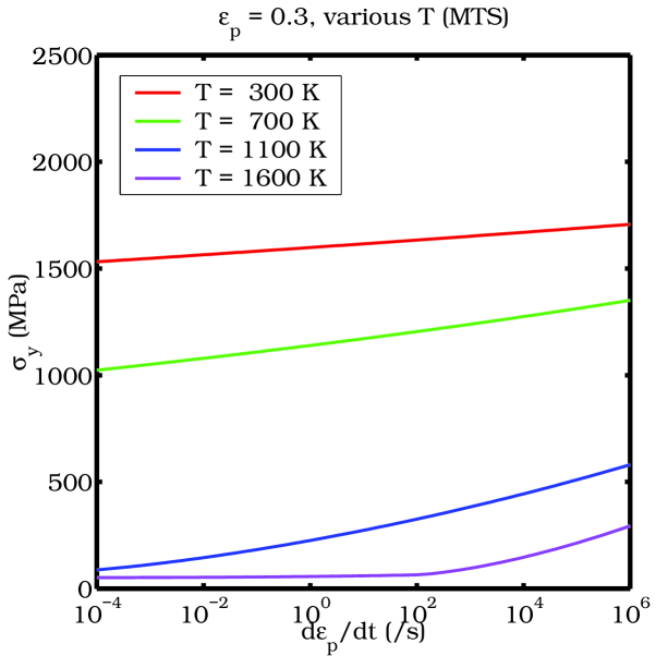
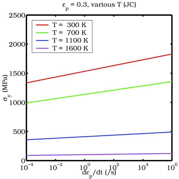
(a) MTS Prediction.                        (b) JC Prediction.

Figure 25: Comparison of MTS and JC predictions of yield stress versus strain rate at various temperatures for $\epsilon_{p}$ = 0.3 .

6.3 Yield stress versus temperature

The temperature dependence of the yield stress for various plastic strains (at a strain rate of 1000 /s) is shown in Figures 26(a) and (b). The sharp change in the value of the yield stress at the phase transition temperature may be problematic for Newton methods used in the determination of the plastic strain rate. We suggest that at temperatures close to the phase transition temperature, the high temperature parameters should be used in numerical computations. The figures show that both the models predict similar rates of temperature dependence of the yield stress.

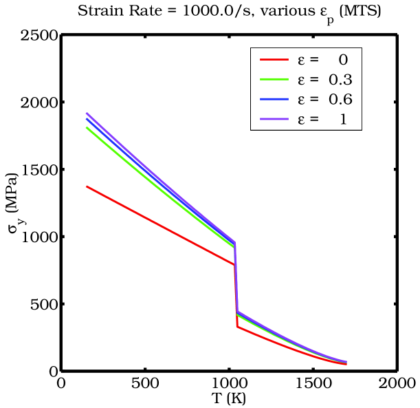
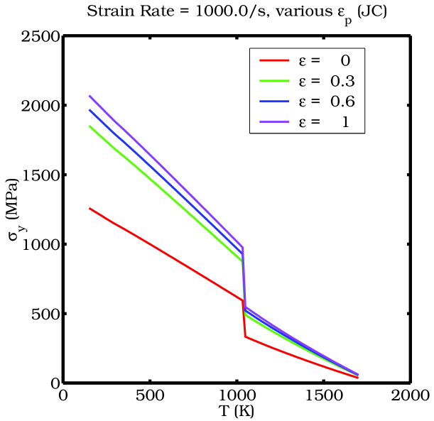
(a) MTS Prediction.                        (b) JC Prediction.

Figure 26: Comparison of MTS and JC predictions of yield stress versus temperature at various plastic strains for $\dot{\epsilon}$ = 1000/s.

The temperature dependence of the yield stress for various strain rates (at a plastic strain of 0.3) is shown in Figures 27(a) and (b). In this case, the MTS model predicts at smaller strain rate effect at low temperatures than the JC model. The strain rate dependence of the yield stress increases with temperature for the MTS model while it decreases with temperature for the JC model. The JC model appears to predict a more realistic behavior because the thermal activation energy for dislocation motion is quite low at high temperatures. However, the MTS model fits high temperature/high strain rate experimental data better than the JC model and we might be observing the correct behavior in the MTS model.

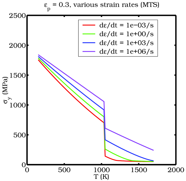
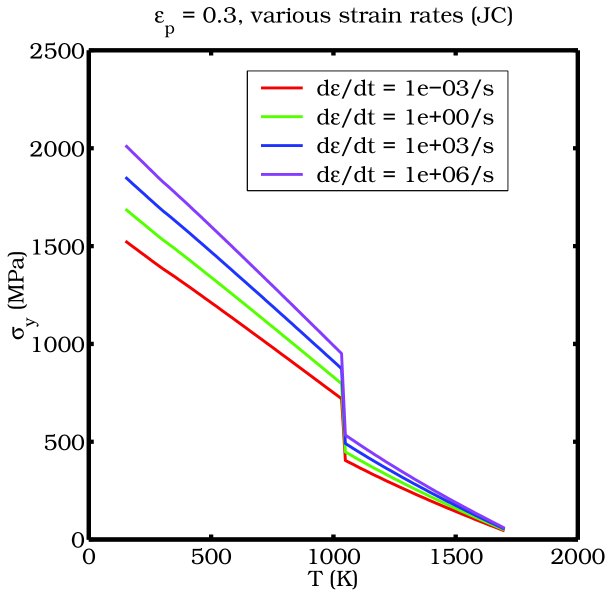
(a) MTS Prediction.                        (b) JC Prediction.

Figure 27: Comparison of MTS and JC predictions of yield stress versus temperature at various strain rates for $\epsilon_{p}$ = 0.3 .

6.4 Taylor impact tests

For further confirmation of the effectiveness of the MTS model, we have simulated three-dimensional Taylor impact tests using the Uintah code (Banerjee [2]). Details of the code, the algorithm used, and the validation process have been discussed elsewhere (Banerjee [2, 3]).

It is well known that the final length of a Taylor impact cylinder scales with the initial velocity. Figure 28 shows some experimental data on the final length of cylindrical Taylor impact specimens as a function of initial velocity. We are interested in temperatures higher than room temperature. For clarity, we have separated the high temperature tests from the room temperature tests by adding an initial internal energy component to the initial kinetic energy density. We have simulated three Taylor tests at three energy levels (marked with crosses on the plot).

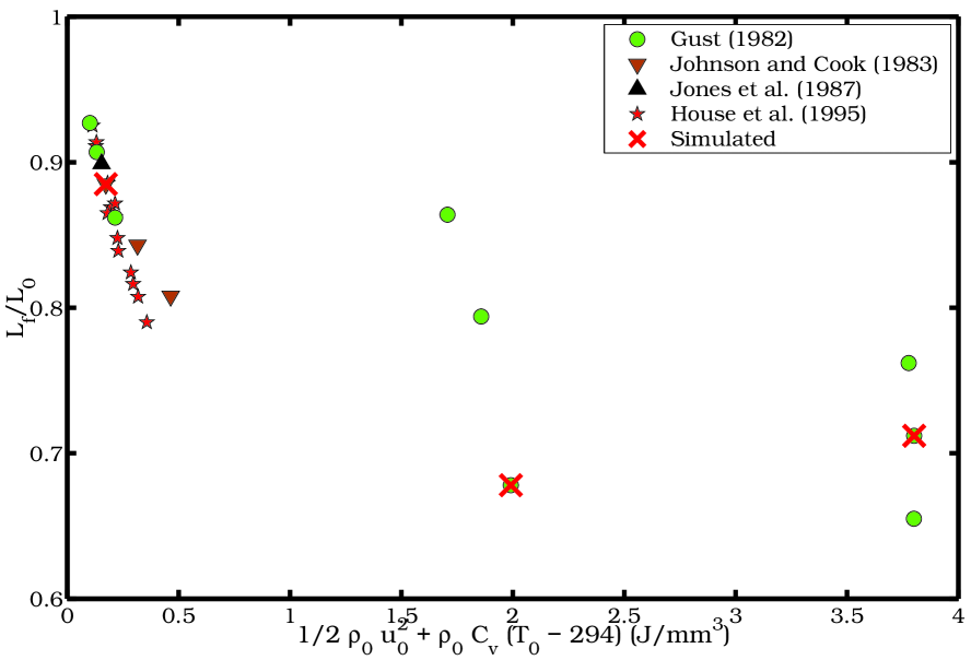
Figure 28: The ratio of the final length to the initial length of Taylor impact specimens as a function of initial energy density. The experimental data are from Gust [19], Johnson and Cook [25], Jones and Gillis [27], and House et al. [23]. The tests that we have simulated are marked with crosses.

The four cases that we have simulated have the following initial conditions:

1. Case 1: $R_{c}$ = 30; $L_{0}$ = 25.4 mm; $D_{0}$ = 7.62 mm; $U_{0}$ = 208 m/s; $T_{0}$ = 298 K; Source Johnson and Cook [25].

2. Case 2: $R_{c}$ = 40; $L_{0}$ = 30.0 mm; $D_{0}$ = 6.0 mm; $U_{0}$ = 312 m/s; $T_{0}$ = 725 K; Source Gust [19].

3. Case 3: $R_{c}$ = 40; $L_{0}$ = 30.0 mm; $D_{0}$ = 6.0 mm; $U_{0}$ = 160 m/s; $T_{0}$ = 1285 K; Source Gust [19].

4. Case 4: $R_{c}$ = 40; $L_{0}$ = 30.0 mm; $D_{0}$ = 6.0 mm; $U_{0}$ = 612 m/s; $T_{0}$ = 725 K;

The MTS model parameters for the $R_{c}$ 30 temper of 4340 steel have been given earlier. The MTS parameters for the $R_{c}$ 40 temper of 4340 steel can be calculated either using the linear fit for various hardness levels (shown in Figure 9) or by a linear interpolation between the $R_{c}$ 38 and the $R_{c}$ 45 values. MTS model parameters at temperatures above 1040 K take the high temperature values discussed earlier. The initial yield stress in the Johnson-Cook model is obtained from the $R_{c}$-$\sigma_{0}$ relation given in Appendix C.

The computed final profiles are compared with the experimental data in Figures 29(a), (b), (c), and (d).

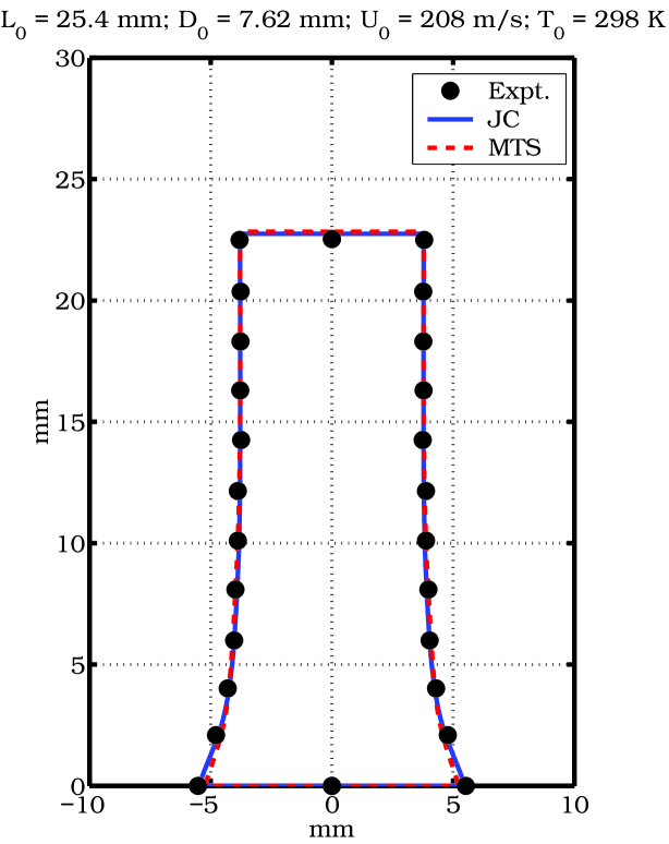
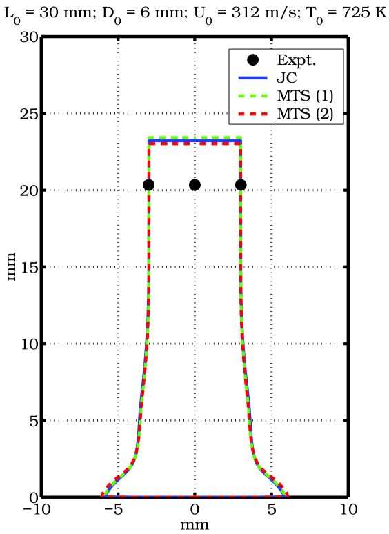
(a) Case 1.                                   (b) Case 2.

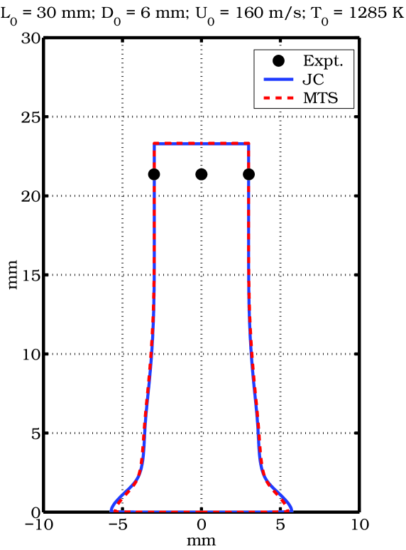
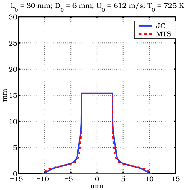
(c) Case 3.                                   (d) Case 4.

Figure 29: Comparison of MTS and JC predictions of final Taylor specimen profiles with experimental results.

For the room temperature test (Figure 29(a)), the Johnson-Cook model accurately predicts the final length, the mushroom diameter, and the overall profile. The MTS model underestimates the mushroom diameter by 0.25 mm. This difference is within experimental variation (see House et al. [23]).

The simulations at 725 K (Figure 29(b)) overestimate the final length of the specimen. The legend shows two MTS predictions for this case - MTS (1) and MTS (2). MTS (1) uses parameters $\sigma_{i}$ and $g_{0i}$ that have been obtained using the fits shown in Figure 9. MTS (2) used parameters obtained by linear interpolation between the $R_{c}$ 38 and $R_{c}$ 45 values. The MTS (2) simulation predicts a final length that is slightly less than that predicted by the MTS (1) and Johnson-Cook models. The mushroom diameter is also slightly larger for the MTS (2) simulation.

The final length of the specimen for Case 2 is not predicted accurately by either model. We have confirmed that this error is not due to discretization (note that volumetric locking does not occur with the explicit Material Point Method used in the simulations). Plots of energy and momentum have also shown that both quantities are conserved in these simulations. The final mushroom diameter is not provided by [19]. However, the author mentions that no fracture was observed in the specimen - discounting a smaller final length due to fracture. In the absence of more extensive high temperature Taylor impact data it is unclear if the error is within experimental variation or due to a fault with the models used.

The third case (Figure 29(c)) was simulated at an initial temperature of 1285 K (above the $\alpha$-$\gamma$ phase transition temperature of iron). The MTS and Johnson-Cook models predict almost exactly the same behavior for this case. The final length is overestimated by both the models. Notice that the final lengths shown in Figure 28 at or near this temperature and for similar initial velocities vary from 0.65 to 0.75 of the initial length. The simulations predict a final length that is approximately 0.77 times the initial length - which is to the higher end of the range of expected final lengths. The discrepancy may be because the models do not predict sufficient strain hardening at these high temperatures.

In all three cases, the predictions from the MTS and the Johnson-Cook models are nearly identical. To determine if any significant difference between the predictions of these models can be observed at higher strain rates, we simulated the geometry of Case 2 with a initial velocity of 612 m/s. The resulting profiles predicted by the MTS and the Johnson-Cook models are shown in Figure 29(d). In this case, the MTS model predicts a slightly wider mushroom than the Johnson-Cook model. The final predicted lengths are almost identical. Interestingly, the amount of strain hardening predicted by the MTS model is smaller than that predicted by the Johnson-Cook model (as can be observed from the secondary bulge in the cylinder above the mushroom). We conclude that the Johnson-Cook and MTS models presented in this paper predict almost identical elastic-plastic behavior in the range of conditions explored. Please note that quite different sets of data were used to determine the parameters of these models and hence the similarity of the results may indicate the underlying accuracy of the parameters.

7 Remarks and Conclusions

We have determined parameters for the Mechanical Threshold Stress model and the Johnson-Cook model for various tempers of 4340 steel. The predictions of the MTS model have been compared with experimental stress-strain data. Yield stresses predicted by the Johnson-Cook and the MTS model have been compared for a range of strain rates and temperatures. Taylor impact tests have been simulated and the predicted profiles have been compared with experimental data.

Some remarks and conclusions regarding this work are given below.

1. The MTS and Johnson-Cook models predict similar stress-strain behaviors over a large range of strain rates and temperatures. Noting that the parameters for these models have been obtained from different sets of experimental data, the similarity of the results, especially in the Taylor test simulations, is remarkable. We suggest that this is an indication of the accuracy of the models and the simulations. However, the Taylor impact tests show that both models predict lower strains at high temperatures than experiments suggest. We are in the process of determining paramters for the Preston-Tonks-Wallace model (Preston et al. [37]) to check if the issue is model dependent.

2. The MTS model parameters are considerably easier to obtain than the Johnson-Cook parameters. However, the MTS simulations of the Taylor impact tests take approximately 1.5 times longer than the Johnson-Cook simulations. This is partly because the shear modulus and melting temperature models are not evaluated in the Johnson-Cook model simulations. Also, the MTS model involves more floating point operations than the Johnson-Cook model. The Johnson-Cook model is numerically more efficient than the MTS model and is preferable for large numerical simulations involving 4340 steel.

3. The Nadal-LePoac shear modulus model and the Burakovsky-Preston-Silbar melting temperature model involve less data fitting and are the suggested models for elastic-plastic simulations over a large range of temperatures and strain rates. The specific heat model that we have presented leads to better predictions of the rate of temperature increase close to the $\alpha$-$\gamma$ phase transition of iron. The shear modulus and melt temperature models are also valid in the range of strain rates of the order of 10⁸ /s. The Mie-Grüneisen equation of state should probably be replaced by a higher order equation of state for extremely high rate processes.

4. The relations between the Rockwell C hardness and the model parameters that have been presented provide reasonable estimates of the parameters. However, more data for the $R_{c}$ 30, 45, and 49 tempers are needed for better estimates for intermediate tempers. There is an anomaly in the strain rate and temperature dependence of the yield strength for $R_{c}$ 50 and higher tempers of 4340 steel. We would suggest that the values for $R_{c}$ 49 steel be used for harder tempers. For tempers below $R_{c}$ 30, the fits discussed earlier provide reasonable estimates of the yield stress.

5. The strain hardening (Voce) rule in the MTS model may be a major weakness of the model and should be replaced with a more physically based approach. The experimental data used to determine the strain hardening rate parameters appear to deviate significantly from Voce behavior is some cases.

6. The determination of the values of $g_{0es}$ and $\sigma_{0es}$ involves a Fisher type modified Arrhenius plot. We have observed that the experimental data for the $R_{c}$ 45 and $R_{c}$ 49 tempers do not tend to reflect an Arrhenius relationship. More experimental data (and information on the variation of the experimental data) are needed to confirm this anomaly.

Appendix A Fisher plot data for $\sigma_{i}$ and $g_{0i}$

Tables 7, 8, 9, and 10 show the Fisher plot data used to calculate $g_{0i}$ and $\sigma_{i}$ for the four tempers of 4340 steel.

Table 7: Fisher plot data used to calculate $g_{0i}$ and $\sigma_{i}$ for 4340 steel of hardness $R_{c}$ 30.

$[k_{b}T/\mu b^{3}\ln(\dot{\epsilon}_{0i}/\dot{\epsilon})]^{1/q_{i}}$	$[(\sigma_{y}-\sigma_{a})/\mu]^{p_{i}}$	$T$ (K)	$\dot{\epsilon}$ (/s)	$\sigma_{y}$ (MPa)	$\mu$ (GPa)
0.08333	0.044658	298	0.002	802.577	79.745
0.0782424	0.0432816	298	0.009	768.052	79.745
0.0700974	0.0425718	298	0.1	750.461	79.745
0.0619864	0.0469729	298	1.1	861.843	79.745
0.0408444	0.0447093	298	570	803.874	79.745
0.0747152	0.0435192	500	604	710.861	72.793
0.122804	0.044074	735	650	648.71	64.706

Table 8: Fisher plot data used to calculate $g_{0i}$ and $\sigma_{i}$ for 4340 steel of hardness $R_{c}$ 38.

$[k_{b}T/\mu b^{3}\ln(\dot{\epsilon}_{0i}/\dot{\epsilon})]^{1/q_{i}}$	$[(\sigma_{y}-\sigma_{a})/\mu]^{p_{i}}$	$T$ (K)	$\dot{\epsilon}$ (/s)	$\sigma_{y}$ (MPa)	$\mu$ (GPa)
0.0775492	0.0563156	258	0.0002	1134.12	81.121
0.0911186	0.0542514	298	0.0002	1057.67	79.745
0.0412876	0.0565499	298	500	1122.38	79.745
0.0375715	0.0576617	298	1500	1154.16	79.745
0.117866	0.0551309	373	0.0002	1048.86	77.164
0.0900788	0.0508976	573	500	857.017	70.281
0.0819713	0.0531021	573	1500	910.012	70.281
0.134713	0.0420956	773	500	597.559	63.398
0.11695	0.0461642	773	2500	678.83	63.398
0.173098	0.0367619	973	1500	448.348	56.515
0.165137	0.037095	973	2500	453.773	56.515
0.237617	0.0263176	1173	1500	261.902	49.632
0.226689	0.0287519	1173	2500	291.972	49.632
0.322911	0.0199969	1373	1500	170.886	42.75
0.30806	0.0220299	1373	2500	189.782	42.75

Table 9: Fisher plot data used to calculate $g_{0i}$ and $\sigma_{i}$ for 4340 steel of hardness $R_{c}$ 45.

$[k_{b}T/\mu b^{3}\ln(\dot{\epsilon}_{0i}/\dot{\epsilon})]^{1/q_{i}}$	$[(\sigma_{y}-\sigma_{a})/\mu]^{p_{i}}$	$T$ (K)	$\dot{\epsilon}$ (/s)	$\sigma_{y}$ (MPa)	$\mu$ (GPa)
0.0514817	0.0645752	173	0.0001	1429.17	84.046
0.0214507	0.0679395	173	1000	1538.34	84.046
0.0934632	0.0611362	298	0.0001	1255.45	79.745
0.038943	0.0683132	298	1000	1473.83	79.745
0.120899	0.062664	373	0.0001	1260.43	77.164
0.0503745	0.0653759	373	1000	1339.85	77.164

Table 10: Fisher plot data used to calculate $g_{0i}$ and $\sigma_{i}$ for 4340 steel of hardness $R_{c}$ 49.

$[k_{b}T/\mu b^{3}\ln(\dot{\epsilon}_{0i}/\dot{\epsilon})]^{1/q_{i}}$	$[(\sigma_{y}-\sigma_{a})/\mu]^{p_{i}}$	$T$ (K)	$\dot{\epsilon}$ (/s)	$\sigma_{y}$ (MPa)	$\mu$ (GPa)
0.0514817	0.0682425	173	0.0001	1548.31	84.046
0.0214507	0.0711498	173	1000	1645.07	84.046
0.0934632	0.0674349	298	0.0001	1446.46	79.745
0.038943	0.0710307	298	1000	1559.63	79.745
0.120899	0.0653628	373	0.0001	1339.46	77.164
0.0503745	0.0694326	373	1000	1461.75	77.164

Appendix B Fisher plot data for $\sigma_{0es}$ and $g_{0es}$

The data used to compute the parameters $\sigma_{0es}$ and $g_{0es}$ are shown in Tables 11, 12, 13, and 14.

Table 11: Fisher plot data used to calculate $g_{0es}$ and $\sigma_{0es}$ for 4340 steel of hardness $R_{c}$ 30.

$[k_{b}T/\mu b^{3}\ln(\dot{\epsilon}_{0es}/\dot{\epsilon})]$	$\ln(\sigma_{es})$	$T_{0}$ (K)	$T_{s}$ (K)	$\dot{\epsilon}$ (/s)	$\sigma_{es}$ (MPa)	$\mu$ (GPa)
$R_{c}$ = 30
0.075541	20.986	298	298	0.002	1300	79.745
0.070454	19.807	298	298	0.009	400	79.745
0.062309	19.989	298	298	0.1	480	79.745
0.054198	19.968	298	298	1.1	470	79.745
0.038728	20.986	298	344	570	1300	78.571
0.064987	20.125	500	532	604	550	71.984
0.10315	19.807	735	758	650	400	64.126

Table 12: Fisher plot data used to calculate $g_{0es}$ and $\sigma_{0es}$ for 4340 steel of hardness $R_{c}$ 38.

$[k_{b}T/\mu b^{3}\ln(\dot{\epsilon}_{0es}/\dot{\epsilon})]$	$\ln(\sigma_{es})$	$T_{0}$ (K)	$T_{s}$ (K)	$\dot{\epsilon}$ (/s)	$\sigma_{es}$ (MPa)	$\mu$ (GPa)
$R_{c}$ = 38
0.07092	21.129	258	258	0.0002	1500	81.121
0.08333	20.986	298	298	0.0002	1300	79.745
0.10779	21.254	373	373	0.0002	1700	77.164
0.036227	20.212	298	320	500	600	79.183
0.075873	20.05	573	591	500	510	69.826
0.11153	19.552	773	785	500	310	63.096
0.037964	20.618	298	371	1500	900	77.886
0.070669	20.367	573	614	1500	700	69.246
0.14023	20.03	973	988	1500	500	56.154
0.098146	20.125	773	815	2500	550	62.342
0.13342	20.088	973	995	2500	530	55.989
0.19164	19.519	1173	1185	1500	300	49.282
0.25895	18.891	1373	1381	1500	160	42.505
0.18261	19.163	1173	1193	2500	210	49.047
0.24641	19.376	1373	1388	2500	260	42.289

Table 13: Fisher plot data used to calculate $g_{0es}$ and $\sigma_{0es}$ for 4340 steel of hardness $R_{c}$ 45.

$[k_{b}T/\mu b^{3}\ln(\dot{\epsilon}_{0es}/\dot{\epsilon})]$	$\ln(\sigma_{es})$	$T_{0}$ (K)	$T_{s}$ (K)	$\dot{\epsilon}$ (/s)	$\sigma_{es}$ (MPa)	$\mu$ (GPa)
$R_{c}$ = 45
0.047192	19.414	173	173	0.0001	270	84.046
0.085675	17.034	298	298	0.0001	25	79.745
0.11082	19.715	373	373	0.0001	365	77.164
0.021177	19.139	173	211	1000	205	83.067
0.034507	18.683	298	327	1000	130	79.004
0.043234	18.826	373	397	1000	150	76.553

Table 14: Fisher plot data used to calculate $g_{0es}$ and $\sigma_{0es}$ for 4340 steel of hardness $R_{c}$ 49.

$[k_{b}T/\mu b^{3}\ln(\dot{\epsilon}_{0es}/\dot{\epsilon})]$	$\ln(\sigma_{es})$	$T_{0}$ (K)	$T_{s}$ (K)	$\dot{\epsilon}$ (/s)	$\sigma_{es}$ (MPa)	$\mu$ (GPa)
$R_{c}$ = 49
0.047192	19.254	173	173	0.0001	230	84.046
0.085675	19.376	298	298	0.0001	260	79.745
0.11082	19.756	373	373	0.0001	380	77.164
0.02075	18.951	173	207	1000	170	83.17
0.035325	19.45	298	334	1000	280	78.826
0.043234	19.45	373	397	1000	280	76.553

Appendix C Johnson-Cook model and parameters

The Johnson-Cook (JC) model (Johnson and Cook [25]) is purely empirical and has the form

$$\sigma_{y}(\epsilon_{p},\dot{\epsilon},T) =\sigma_{0}\left[1+\cfrac{B}{\sigma_{0}}(\epsilon_{p})^{n}\right]\left[1+C\ln(\dot{\epsilon}^{*})\right]\left[1-(T^{*})^{m}\right]$$ (26)

$$\dot{\epsilon}^{*} =\cfrac{\dot{\epsilon}}{\dot{\epsilon}_{0}};\quad T^{*}=\cfrac{(T-T_{r})}{(T_{m}-T_{r})}$$ (27)

where $\sigma_{0}$ is the yield stress at zero plastic strain, and $(B,C,n,m)$ are material constants, $\dot{\epsilon}_{0}$ is a reference strain rate, and $T_{r}$ is a reference temperature.

The value of $\sigma_{0}$ for 4340 steel in the Johnson-Cook model varies with the temper of the steel. We have fit the yield stress versus $R_{c}$ hardness curve for 4340 steel from the ASM handbook [21] to determine the value of $\sigma_{0}$ for various tempers. The equation for the fit is

$$\sigma_{0}=\exp(A_{1}R_{c}+A_{2})~{}~{}\text{(MPa)}$$ (28)

where $A_{1}=$ 0.0355 ln(MPa), $A_{2}=$ 5.5312 ln(MPa), and $R_{c}$ is the Rockwell-C hardness of the steel. The value of $B/\sigma_{0}=$ 0.6339 is assumed to be a constant for all tempers. The strain hardening exponent ($n$) is 0.26 and the strain rate dependence parameter ($C$) is 0.014, for all tempers. The reference strain rate $\dot{\epsilon}_{0}$ is 1 /s. For temperatures less than 298 K, thermal softening is assumed to be linear and the parameter $m$ takes a value of 1. Above 298 K and lower than 1040 K, $m$ is assumed to be 1.03, and beyond 1040 K, $m$ is taken as 0.5 (Lee and Yeh [33]). The reference temperature ($T_{r}$) is 298 K and the melt temperature ($T_{m}$) is kept fixed at 1793 K. These parameters provide a reasonable fit to the experimental data presented earlier in the context of the MTS model.

References

- Bancroft et al. [1956] Bancroft, D., Peterson, E. L., Minshall, S., 1956. Polymorphism of iron at high pressure. J. Appl. Phys 27 (3), 291–298.
- Banerjee [2005a] Banerjee, B., 2005a. Simulation of impact and fragmentation with the material point method. In: Proc. 11th International Conference on Fracture. Turin, Italy.
- Banerjee [2005b] Banerjee, B., 2005b. Validation of UINTAH: Taylor impact and plasticity models. In: Proc. 2005 Joint ASME/ASCE/SES Conference on Mechanics and Materials (McMat 2005). Baton Rouge, LA.
- Barker and Hollenbach [1974] Barker, L. M., Hollenbach, R. E., 1974. Shock wave study of the phase transition in iron. J. Appl. Phys. 45 (11), 4872–4887.
- Brown et al. [2000] Brown, J. M., Fritz, J. N., Hixson, R. S., 2000. Hugoniot data for iron. J. Appl. Phys. 88 (9), 5496–5498.
- Brown et al. [1996] Brown, W. F., Mindlin, H., Ho, C. Y., 1996. Aerospace Structural Metals Handbook: Volume 1: Code 1206. CINDAS/USAF CRDA Handbooks Operation, Purdue University, West Lafayette, IN.
- Burakovsky and Preston [2000] Burakovsky, L., Preston, D. L., 2000. Analysis of dislocation mechanism for melting of elements. Solid State Comm. 115, 341–345.
- Burakovsky et al. [2000a] Burakovsky, L., Preston, D. L., Silbar, R. R., 2000a. Analysis of dislocation mechanism for melting of elements: pressure dependence. J. Appl. Phys. 88 (11), 6294–6301.
- Burakovsky et al. [2000b] Burakovsky, L., Preston, D. L., Silbar, R. R., 2000b. Melting as a dislocation-mediated phase transition. Phys. Rev. B 61 (22), 15011–15018.
- Caillard and Martin [2003] Caillard, D., Martin, J. L., 2003. Thermally Activated Mechanisms in Crystal Plasticity. Pergamon, Amsterdam.
- Chen and Gray [1996] Chen, S. R., Gray, G. T., 1996. Constitutive behavior of tantalum and tantalum-tungsten alloys. Metall. Mater. Trans. A 27A, 2994–3006.
- Chi et al. [1989] Chi, Y. C., Lee, S., Cho, K., Duffy, J., 1989. The effect of tempering and test temperature on the dynamic fracture initiation behavior of an AISI 4340 VAR steel. Mat. Sci. Eng. A114, 105–126.
- Cottrell and Bilby [1949] Cottrell, A. H., Bilby, B. A., 1949. Dislocation theory of yielding and strain aging of iron. Proc. Phys. Soc. London A 62, 49–62.
- Follansbee and Kocks [1988] Follansbee, P. S., Kocks, U. F., 1988. A constitutive description of the deformation of copper based on the use of the mechanical threshold stress as an internal state variable. Acta Metall. 36, 82–93.
- Fukuhara and Sanpei [1993] Fukuhara, M., Sanpei, A., 1993. Elastic moduli and internal friction of low carbon and stainless steels as a function of temperature. ISIJ International 33 (4), 508–512.
- Goto et al. [2000a] Goto, D. M., Bingert, J. F., Chen, S. R., Gray, G. T., Garrett, R. K., 2000a. The mechanical threshold stress constitutive-strength model description of HY-100 steel. Metallurgical and Materials Transactions A 31A, 1985–1996.
- Goto et al. [2000b] Goto, D. M., Bingert, J. F., Reed, W. R., Garrett, R. K., 2000b. Anisotropy-corrected MTS constitutive strength modeling in HY-100 steel. Scripta Mater. 42, 1125–1131.
- Guinan and Steinberg [1974] Guinan, M. W., Steinberg, D. J., 1974. Pressure and temperature derivatives of the isotropic polycrystalline shear modulus for 65 elements. J. Phys. Chem. Solids 35, 1501–1512.
- Gust [1982] Gust, W. H., 1982. High impact deformation of metal cylinders at elevated temperatures. J. Appl. Phys. 53 (5), 3566–3575.
- Gust et al. [1979] Gust, W. H., Steinberg, D. J., Young, D. A., 1979. Hugoniot parameters to 320 GPa for three types of steel. High Temp. High Pres. 11, 271–280.
- Handbook [1978] Handbook, A., 1978. American Society of Metals Handbook: Volume 1. American Society of Metals, New York.
- Hanson [2005] Hanson, K. M., 2005. Inference about the plastic behavior of materials from experimental data. In: Hanson, K. M., Hemez, F. M. (Eds.), Sensitivity Analysis of Model Output. Los Alamos Research Library, Los Alamos, NM, pp. 126–136.
- House et al. [1995] House, J. W., Lewis, J. C., Gillis, P. P., Wilson, L. L., 1995. Estimation of the flow stress under high rate plastic deformation. Int. J. Impact Engng. 16 (2), 189–200.
- Jansen et al. [1984] Jansen, H. J. F., Hathaway, K. B., Freeman, A. J., 1984. Structural properties of ferromagnetic bcc iron: A failure of the local-spin-density approximation. Phys. Rev. B 30 (10), 6177–6179, lattice constant for bcc iron.
- Johnson and Cook [1983] Johnson, G. R., Cook, W. H., 1983. A constitutive model and data for metals subjected to large strains, high strain rates and high temperatures. In: Proc. 7th International Symposium on Ballistics. pp. 541–547.
- Johnson and Cook [1985] Johnson, G. R., Cook, W. H., 1985. Fracture characteristics of three metals subjected to various strains, strain rates, temperatures and pressures. Int. J. Eng. Fract. Mech. 21, 31–48.
- Jones and Gillis [1987] Jones, S. E., Gillis, P. P., 1987. On the equation of motion of the undeformed section of a Taylor impact specimen. J. Appl. Phys. 61 (2), 499–502.
- Katz et al. [1959] Katz, S., Doran, D. G., Curran, D. R., 1959. Hugoniot equation of state of aluminum and steel from oblique shock measurements. J. Appl. Phys. 30 (4), 568–576.
- Kocks [2001] Kocks, U. F., 2001. Realistic constitutive relations for metal plasticity. Materials Science and Engrg. A317, 181–187.
- Kocks et al. [1975] Kocks, U. F., Argon, A. S., Ashby, M. F., 1975. Thermodynamics and Kinetics of Slip. Pergamon Press, Oxford.
- Larson and Nunes [1961] Larson, F. R., Nunes, J., 1961. Low temperature flow and fracture tension properties of heat treated SAE 4340 steel. Trans. ASM 53, 663–682.
- Lederman et al. [1974] Lederman, F. L., Salamon, M. B., Shacklette, L. W., 1974. Experimental verification of scaling and test of the universality hypothesis from specific heat data. Phys. Rev. B 9 (7), 2981–2988.
- Lee and Yeh [1997] Lee, W.-S., Yeh, G.-W., 1997. The plastic deformation behavior of AISI 4340 alloy steel subjected to high temperature and high strain rate loading conditions. J. Mater. Proc. Tech. 71, 224–234.
- McQueen et al. [1970] McQueen, R. G., Marsh, S. P., Taylor, J. W., Fritz, J. N., Carter, W. J., 1970. The equation of state of solids from shock wave studies. In: Kinslow, R. (Ed.), High Velocity Impact Phenomena. Academic Press, New York, pp. 294–417.
- Nadal and Le Poac [2003] Nadal, M.-H., Le Poac, P., 2003. Continuous model for the shear modulus as a function of pressure and temperature up to the melting point: analysis and ultrasonic validation. J. Appl. Phys. 93 (5), 2472–2480.
- Nicholas [1981] Nicholas, T., 1981. Tensile testing of materials at high rates of strain. Experimental Mechanics 21, 117–185.
- Preston et al. [2003] Preston, D. L., Tonks, D. L., Wallace, D. C., 2003. Model of plastic deformation for extreme loading conditions. J. Appl. Phys. 93 (1), 211–220.
- Ravichandran et al. [2001] Ravichandran, G., Rosakis, A. J., Hodowany, J., Rosakis, P., 2001. On the conversion of plastic work into heat during high-strain-rate deformation. In: Proc. , 12th APS Topical Conference on Shock Compression of Condensed Matter. American Physical Society, pp. 557–562.
- Shacklette [1974] Shacklette, L. W., 1974. Specific heat and resistivity of iron near its Curie point. Phys. Rev. B 9 (9), 3789–3792.
- Steinberg et al. [1980] Steinberg, D. J., Cochran, S. G., Guinan, M. W., 1980. A constitutive model for metals applicable at high-strain rate. J. Appl. Phys. 51 (3), 1498–1504.
- Tanimura and Duffy [1986] Tanimura, S., Duffy, J., 1986. Strain rate effects and temperature history effects for three different tempers of 4340 VAR steel. Int. J. Plasticity 2, 21–35.
- Varshni [1970] Varshni, Y. P., 1970. Temperature dependence of the elastic constants. Physical Rev. B 2 (10), 3952–3958.
- Wallace et al. [1960] Wallace, D. C., Sidles, P. H., Danielson, G. C., 1960. Specific heat of high purity iron by a pulse heating method. J. Appl. Phys. 31 (1), 168–176.
- Wilkins [1999] Wilkins, M. L., 1999. Computer Simulation of Dynamic Phenomena. Springer-Verlag, Berlin.
- Williams et al. [1987] Williams, Q., Jeanloz, R., Bass, J., Svendsen, B., Ahrens, T. J., 1987. The melting curve of iron to 250 gigapascals: a constraint of the temperature at earth’s center. Science 236, 181–182.
- Yoo et al. [1993] Yoo, C. S., Holmes, N. C., Ross, M., 1993. Shock temperatures and melting of iron at earth core conditions. Phys. Rev. Lett. 70 (25), 3931–3934.
- Zocher et al. [2000] Zocher, M. A., Maudlin, P. J., Chen, S. R., Flower-Maudlin, E. C., 2000. An evaluation of several hardening models using Taylor cylinder impact data. In: Proc. , European Congress on Computational Methods in Applied Sciences and Engineering. ECCOMAS, Barcelona, Spain.