Two-band Fluctuation Exchange Study on the Superconductivity of $\beta^{\prime}$-(BEDT-TTF)₂ICl₂ under High Pressure.

Abstract

We study the pressure dependence of the superconducting transition temperature of an organic superconductor $\beta^{\prime}$-(BEDT-TTF)₂ICl₂ by applying the fluctuation exchange method to the Hubbard model on the original two-band lattice at $3/4$-filling rather than the single band model in the strong dimerization limit. Our study is motivated by the fact that hopping parameters evaluated from a first-principles study suggest that the dimerization of the BEDT-TTF molecules is not so strong especially at high pressure. Solving the linearized Eliashberg’s equation, a d_xy-wave-like superconducting state with realistic values of $T_{c}$ is obtained in a pressure regime somewhat higher than the actual experimental result. These results are similar to those obtained within the single band model in the previous study by Kino et al. We conclude that the resemblance to the dimer limit is due to a combination of a good Fermi surface nesting, a large density of states near the Fermi level, and a moderate dimerization, which cooperatively enhance electron correlation effects and also the superconducting $T_{c}$.

1 Introduction

Over the past few decades, a considerable amount of studies have been performed on organic conductors both experimentally and theoretically. Especially, the occurrence of unconventional superconductivity in these materials, where low dimensionality and/or strong electron correlation may be playing an important role, has become one of the fascinating issues in condensed matter physics.[1]

The title material of this paper, $\beta^{\prime}$-(BEDT-TTF)₂ICl₂ is a charge transfer organic material which consists of cation BEDT-TTF (abbreviated as ET) molecule layers and anion ICl₂ layers. This material is a paramagnetic insulator at room temperature and ambient pressure, and becomes an antiferromagnetic (AF) insulator below the Néel temperature $T_{N}=22$ K. Regarding the electronic structure, since two ET molecules are packed in a unit cell as shown in Fig. 1(a) with 0.5 holes per ET molecule, it is a $3/4$-filled two-band system. Moreover, in the $\beta^{\prime}$-type arrangement of the ET molecules, which is rather modified from the $\beta$-type because of the small size of the anion ICl₂, ET molecules form dimers in the $p1$ direction, which opens up a gap between the two bands. Thus, only the anti-bonding band intersects the Fermi level, so that it may be possible to look at the the system as a half-filled single band system. At ambient pressure, this picture is supported by the fact that system becomes an insulator despite the band being 3/4-filled.

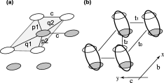
Figure 1: Schematic illustration of the ET molecule layer. (a) The original two band lattice. A small oval represents an ET molecule. $p1$, $p2$, $\cdots$ stand for the hopping integrals $t(p1)$, $t(p2)$, $\cdots$. The shaded portion denotes the unit cell. (b) The effective single band lattice in the dimer limit with effective hoppings $t_{0}$, $t_{1}$, and $t_{2}$.

Recently, superconductivity has been found in this material under high pressure (above 8.2 GPa) by Taniguchi et al. It has the highest transition temperature $T_{c}$ (=$T_{c}^{\rm max}=14.2$ K at $p=8.2$ GPa ) among all the molecular charge-transfer salts. [2] Since the superconducting phase seems to sit next to the antiferromagnetic insulating phase in the pressure-temperature phase diagram, there is a possibility that the pairing is due to AF spin fluctuations. In fact, Kino et al. have calculated $T_{c}$ and the Néel temperature $T_{N}$ using the fluctuation exchange (FLEX)[3] method on an effective single-band Hubbard model at $1/2$-filling, namely the ’dimer model’ obtained in the strong dimerization limit(Fig. 1(b)).[4, 5] In their study, the hopping parameters of the original two band lattice are determined by fitting the tight binding dispersion to those obtained from first principles calculation[6], and the hopping parameters of the effective one band lattice are obtained from a certain transformation. The obtained phase diagram is qualitatively similar to the experimental one although the superconducting phase appears in a higher pressure regime.

Nevertheless, we believe that it is necessary to revisit this problem using the original two-band lattice due to the following reasons. (i)If we look into the values of the hopping integrals of the original two-band lattice, the dimerization is not so strong, and in fact the gap between the bonding and the antibonding bands is only $10$ percent of the total band width at $8$ GPa. (ii) The effective on-site repulsion in the dimer model is a function of hopping integral and thus should also be a function of pressure. [7] (iii) It has been known that assuming the dimerization limit can result in crucial problems as seen in the studies of $\kappa$-(ET)₂X, in which the dimer model gives $d_{x^{2}-y^{2}}$-wave pairing with a moderate $T_{c}$, while in the original four-band lattice, $d_{x^{2}-y^{2}}$ and $d_{xy}$-wave pairings are nearly degenerate with, if any, a very low $T_{c}$. [9, 8] Note that in the case of $\kappa$-(BEDT-TTF)₂X, the band gap between the bonding and the antibonding band is more than 20 % of the total band width,[10] which is larger than that in the title compound.

In the present paper, we calculate $T_{c}$ and the gap function by applying the two-band version of FLEX for the Hubbard model on the two-band lattice at $3/4$-filling using the hopping parameters determined by Miyazaki et al. We obtain finite values of $T_{c}$ in a pressure regime similar to those in the single band approach. The present situation is in sharp contrast with the case of $\kappa$-(ET)₂X in that moderate values of $T_{c}$ (or we should say “high $T_{c}$” in the sense mentioned in §4.4) are obtained even in a $3/4$-filled system, where electron correlation effects are, naively speaking, not expected to be strong compared to true half-filled systems. The present study suggests that the coexistence of a good Fermi surface nesting, a large density of states and a moderate (not so weak) dimerization cooperatively enhances electron correlation effects and leads to results similar to those in the dimer limit. We conclude that these factors that enhance correlation effects should also be the very origin of the high $T_{c}$ itself of the title material.

2 Formulation

In the present study, we adopt a standard Hubbard Hamiltonian having two sites in a unit cell, where each site corresponds to an ET molecule. The kinetic energy part of the Hamiltonian is written as

$${\cal H}_{\rm kin} = \sum_{i,\sigma}\biggl{[}t(c)\Big{(}c_{(i_{x},i_{y}+1),\sigma}^{\dagger}c_{(i_{x},i_{y}),\sigma}$$ (1)

$$+ d_{(i_{x},i_{y}+1),\sigma}^{\dagger}d_{(i_{x},i_{y}),\sigma}\Big{)}$$

$$+ t(q1)d_{(i_{x}-1,i_{y}+1),\sigma}^{\dagger}c_{(i_{x},i_{y}),\sigma}$$

$$+ t(q2)d_{(i_{x},i_{y})\sigma}^{\dagger}c_{(i_{x},i_{y}),\sigma}$$

$$+ t(p1)d_{(i_{x},i_{y}+1),\sigma}^{\dagger}c_{(i_{x},i_{y}),\sigma}$$

$$+ t(p2)d_{(i_{x}-1,i_{y}),\sigma}^{\dagger}c_{(i_{x},i_{y}),\sigma}$$

$$+ {\rm h.c}-\mu\biggr{]},$$

where $c_{i,\sigma}$ and $d_{i,\sigma}$ are annihilation operators of electrons with spin $\sigma$ at the two different sites in the $i$-th unit cell, and $\mu$ represents chemical potential. $t(p1)$, $t(p2)$, $\cdots$ are the hopping parameters in the $p1$, $p2$, $\cdots$ directions, respectively.

The interaction part is

$${\cal H}_{\rm int} = U\sum_{i,\sigma}\left(n_{i,\sigma}^{c}n_{i,\sigma}^{c}+n_{i,\sigma}^{d}n_{i,\sigma}^{d}\right),$$ (2)

where $U$ is the on-site electron-electron interaction, and $n_{i,\sigma}^{c}=c_{i,\sigma}^{\dagger}c_{i,\sigma}$ and $n_{i,\sigma}^{d}=d_{i,\sigma}^{\dagger}d_{i,\sigma}$ are the number operators. The pressure effect on the electronic structure is introduced through the hopping parameters within this model. As we have mentioned above, we use the hopping parameters determined by Miyazaki et al.[6] as shown in Table.1, which well reproduce the results of the first principles calculation. For pressures higher than $12$ GPa, which is the highest pressure where the first principles calculation have been carried out, the values of the hopping integrals are obtained by linear extrapolation as in the previous study.

In the present study, we have employed the two-band version of the fluctuation exchange (FLEX) approximation to obtain the Green’s function and the normal self-energy. For later discussions, let us briefly review the FLEX method, which is a kind of self-consistent random phase approximation (RPA). Since FLEX can take large spin fluctuations into account, these methods have been applied to the studies of high-$T_{c}$ cuprates and other organic superconductors.

The (renormalized) thermal Green’s function $G(\mbox{\boldmath{$k$}},\varepsilon)$ is given by the Dyson’s equation,

$$G^{-1}(\mbox{\boldmath{$k$}},\varepsilon_{n})=G_{0}^{-1}(\mbox{\boldmath{$k$}},\varepsilon_{n})-\Sigma(\mbox{\boldmath{$k$}},\varepsilon_{n}),$$ (3)

where $\varepsilon_{n}=(2n+1)\pi T$ is the Matsubara frequency with $n=0,\pm 1,\pm 2,\cdots$. $G_{0}(\mbox{\boldmath{$k$}},\varepsilon_{n})$ is the unperturbed thermal Green’s function and $\Sigma(\mbox{\boldmath{$k$}},\varepsilon_{n})$ is the normal self-energy, which has an effect of suppressing $T_{c}$.

Using $G(\mbox{\boldmath{$k$}},\varepsilon_{n})$ obtained by solving eq.(3), the irreducible susceptibility $\chi_{0}(\mbox{\boldmath{$q$}},\omega_{m})$ is given as

$$\chi_{0}(\mbox{\boldmath{$q$}},\omega_{m})=-\frac{1}{N}\sum_{k,n}G(\mbox{\boldmath{$k$}}+\mbox{\boldmath{$q$}},\omega_{m}+\varepsilon_{n})G(\mbox{\boldmath{$k$}},\varepsilon_{n}),$$ (4)

where $\omega_{m}$ is the Matsubara frequency for bosons with $m=0,\pm 1,\pm 2,\cdots$ and $N$ is the number of $k$-point meshes. By collecting RPA-type diagrams, the effective interaction $V^{(1)}$ and the singlet pairing interaction $V^{(2)}$ are obtained as

$$V^{(1)}(\mbox{\boldmath{$q$}},\omega_{m}) = -\frac{3}{2}U^{2}\chi_{s}(\mbox{\boldmath{$q$}},\omega_{m})-\frac{1}{2}U^{2}\chi_{c}(\mbox{\boldmath{$q$}},\omega_{m})$$ (5)

$$V^{(2)}(\mbox{\boldmath{$q$}},\omega_{m}) = U+\frac{3}{2}U^{2}\chi_{s}(\mbox{\boldmath{$q$}},\omega_{m})-\frac{1}{2}U^{2}\chi_{c}(\mbox{\boldmath{$q$}},\omega_{m}),$$ (6)

where $\chi_{s}$,$\chi_{c}$ are spin and charge susceptibilities, respectively, given as

$$\chi_{s,c}(\mbox{\boldmath{$q$}},\omega_{m})=\frac{\chi_{0}(\mbox{\boldmath{$q$}},\omega_{m})}{1\mp U\chi_{0}(\mbox{\boldmath{$q$}},\omega_{m})}.$$ (7)

Then the normal self-energy is given by

$$\Sigma(\mbox{\boldmath{$k$}},\varepsilon_{n})=-\frac{T}{N}\sum_{q,m}G(\mbox{\boldmath{$k$}}-\mbox{\boldmath{$q$}},\varepsilon_{n})\left[V^{(1)}(\mbox{\boldmath{$q$}},\omega_{m})-U^{2}\chi_{0}(\mbox{\boldmath{$q$}},\omega_{m})\right].$$ (8)

The obtained self-energy $\Sigma(\mbox{\boldmath{$k$}},\varepsilon_{n})$ is fed back into the Dyson’s equation eq.(3), and by repeating these procedures, the self-consistent $G(\mbox{\boldmath{$k$}},\varepsilon_{n})$ is obtained.

Table 1: Pressure dependence of the hopping parameters of $\beta^{\prime}$-(ET)₂ICl₂ determined by Miyazaki and Kino. (ref.Miyazaki)

P	$t(p1)$	$t(p2)$	$t(q1)$	$t(q2)$	$t(c)$
0 (GPa)	-0.181 (eV)	0.0330	-0.106	-0.0481	-0.0252
4	-0.268	0.0681	-0.155	-0.0947	-0.0291
8	-0.306	0.0961	-0.174	-0.120	-0.0399
12	-0.313	0.142	-0.195	-0.122	-0.0347
16	-0.320	0.188	-0.216	-0.124	-0.0295

In the two-band version of FLEX, $G(\mbox{\boldmath{$k$}},\varepsilon_{n})$, $\chi_{0}$, $\chi_{s,c}$, $\Sigma(\mbox{\boldmath{$k$}},\omega_{m})$ become $2\times 2$ matrices, e.g. $G_{\alpha\beta}$, where $\alpha$ and $\beta$ denote one of the two sites in a unit cell.

Once $G_{\alpha\beta}(\mbox{\boldmath{$k$}},\varepsilon_{n})$ and $V_{\alpha\beta}^{(2)}$ are obtained by FLEX, we can calculate $T_{c}$ by solving the linearized Eliashberg’s equation as follows,

$$\lambda\phi_{\alpha\beta}(\mbox{\boldmath{$k$}},\varepsilon_{n})=-\frac{T}{N}\sum_{k^{\prime},m,\alpha^{\prime},\beta^{\prime}}V_{\alpha\beta}^{(2)}(\mbox{\boldmath{$k$}}-\mbox{\boldmath{$k$}}^{\prime},\varepsilon_{n}-\varepsilon_{m})$$

$$\times G_{\alpha\alpha^{\prime}}(\mbox{\boldmath{$k$}}^{\prime},\varepsilon_{m})G_{\beta\beta^{\prime}}(-\mbox{\boldmath{$k$}}^{\prime},-\varepsilon_{m})\phi_{\alpha^{\prime}\beta^{\prime}}(\mbox{\boldmath{$k$}}^{\prime},\varepsilon_{m}),$$ (9)

where $\phi(\mbox{\boldmath{$k$}})$ is the superconducting gap function. The transition temperature $T_{c}$ is determined as the temperature where the eigenvalue $\lambda$ reaches unity.

In the actual calculation, we use $64\times 64$ $k$-point meshes and $16384$ Matsubara frequencies in order to ensure convergence at the lowest temperature studied ($T/|t(p1)|=0.002$). The bandfilling (the number of electrons per site) is fixed at $n=1.5$.

When $U\chi_{0}(\mbox{\boldmath{$q$}},\omega_{m}=0)=1$, the spin susceptibility diverges and a magnetic ordering takes place. In the FLEX calculation in two-dimensional systems, Mermin-Wagner’s theorem is satisfied,[11, 12] so that $U\chi_{0}(\mbox{\boldmath{$q$}},\omega_{m}=0)<1$, namely true magnetic ordering does not take place. However, this is an artifact of adopting a purely two-dimensional model, while the actual material is quasi two dimensional. Thus, in the present study, we assume that if there were a weak three dimensionality, a magnetic ordering with wave vector $q$ would occur when

$$\max_{q}\left\{U\chi_{0}(\mbox{\boldmath{$q$}},\omega_{n}=0)>0.995\right\},$$ (10)

is satisfied in the temperature range where $\lambda<1$. Therefore we do not calculate $T_{c}$ in such a parameter regime. [13]

3 Results

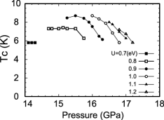
Figure 2: Transition temperature $T_{c}$ as functions of pressure for several values of $U$.

Now we move on to the results. Figure 2 shows the pressure dependence of $T_{c}$ obtained for several values of $U$. Since our calculation is restricted to temperatures above $\sim$ 6 K, $T_{c}$ is obtained within that temperature range. At pressure lower than the superconducting regime, the system is in the AF phase in the sense we mentioned in §2. The maximum $T_{c}$ obtained is $T_{c}^{\rm max}=8.7$ K (at $15.5$ GPa for $U=0.9$ eV, and $16.0$ GPa for $U=1.0$ eV), which is somewhat smaller than the experimental maximum value of $T_{c}$, but can be considered as fairly realistic. The overall phase diagram is qualitatively similar to the experimental phase diagram, but the pressure range in which superconductivity occurs is above $\sim 14$ GPa and extends up to $\sim 17$ GPa or higher, is higher than the experimental results. These results are similar to those obtained within the dimer model approach.[4]

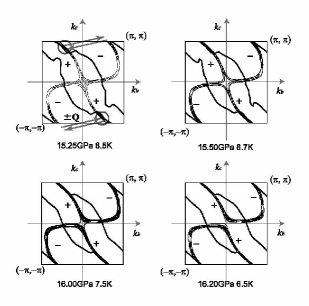
Figure 3: Contour plots of $|G(\mbox{\boldmath{$k$}})|^{2}$ and the nodes of the superconducting gap function $\phi(\mbox{\boldmath{$k$}})$ for $U=0.9$ eV at $p=15.25$, $15.5$, $16.0$, and $16.2$ GPa. At $p=15.25$ GPa, $\phi(\mbox{\boldmath{$k$}})\phi(\mbox{\boldmath{$k$}}+\mbox{\boldmath{$Q$}})$ is positive at the circled portions of the Fermi surface.

Figure 3 shows the nodal lines of $\phi(\mbox{\boldmath{$k$}})$ and the contour plots of $|G(\mbox{\boldmath{$k$}})|^{2}$ for several values of pressure with $U=0.9$ eV. In the plots of $|G(\mbox{\boldmath{$k$}})|^{2}$, the center of the densely bundled contour lines correspond to the ridges of $|G(\mbox{\boldmath{$k$}})|^{2}$ and thus the Fermi surface, while the thickness of these bundles can be considered as a measure for the density of states near the Fermi level, namely, the thicker these bundles, the larger number of states lie near the Fermi level. With increasing pressure, the Fermi surface changes its topology from a one dimensional one open in the $k_{c}$ direction to a closed two dimensional one around $(0,\pi)$. Again like in the single band approach, the pairing symmetry is $d_{xy}$-wave-like in the sense that $\phi(\mbox{\boldmath{$k$}})$ changes its sign as ($+-+-$) along the Fermi surface and the nodes of the gap intersect the Fermi surfaces near $x$ and $y$ axes. The peak position of the spin susceptibility $\chi_{s}(\mbox{\boldmath{$q$}})$ shown in Fig. 4, which should correspond to the nesting vector of the Fermi surface, stays around $\mbox{\boldmath{$Q$}}=(\pi,\pi/4)$ regardless of the pressure. This vector $Q$ bridges the portion of the Fermi surface with $\phi({\mbox{\boldmath{$k$}}})<0$ and $\phi(\mbox{\boldmath{$k$}}+\mbox{\boldmath{$Q$}})>0$, which is the origin of the $d_{xy}$-wave like gap.

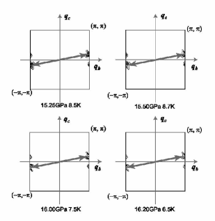
Figure 4: Contour plots of the spin susceptibility $\chi_{s}(\mbox{\boldmath{$q$}})$ for the same values of $U$ and $p$ as in Fig. 3.

4 Discussion

In this section, we physically interpret some of our calculation results.

4.1 Pressure dependence of $T_{c}$ at fixed values of $U$

For fixed values of $U$, $T_{c}$ tends to be suppressed at high pressure as seen in Fig. 2. This can be explained as follows. We have seen in Fig. 4 that the peak position of the spin susceptibility does not depend on pressure, but the peak value itself decreases with pressure for fixed values of $U$ as shown in Fig. 6. This is because the nesting of the Fermi surface becomes degraded due to the dimensional crossover of the Fermi surface mentioned previously. Consequently, the pairing interaction $V^{(2)}$ (nearly proportional to the spin susceptibility) becomes smaller, so that $T_{c}$ becomes lower, with increasing pressure.

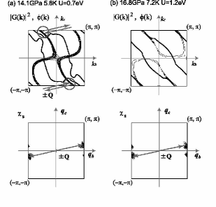
Figure 5: Contour plots of $|G(\mbox{\boldmath{$k$}})|^{2}$, the nodes of the gap function, and the spin susceptibility at (a)$U=0.7$ eV, $p=14.1$ GPa. (b)$U=1.2$ eV,$p=17.2$ GPa. At the circled portions of the Fermi surface, $\phi(\mbox{\boldmath{$k$}})\phi(\mbox{\boldmath{$k$}}+\mbox{\boldmath{$Q$}})$ is positive.

For $U=0.9$ eV (and possibly for $U=0.8$ eV), $T_{c}$ is slightly suppressed also at low pressure, so that a optimum pressure exists. This may be due to the fact that at low pressure, $Q$ (spin susceptibility peak position) bridges some portions of the Fermi surface that has the same sign of the gap (Fig. 3(a)). In fact, this tendency of $Q$ bridging the same gap sign is found to be even stronger for lower values of pressure as seen in Fig. 5(a), while at higher pressure, the nodes of the gap run along the Fermi surface so as to suppress this tendency (Fig. 5(b)). We will come back to this point in §4.3.

4.2 Pressure dependence of the maximum $T_{c}$ upon varying $U$

As can be seen from Fig. 2, for each value of pressure, there exists an optimum value of $U(=U_{\rm opt})$ which maximizes $T_{c}$ . In this subsection, let us discuss the pressure dependence of this optimized $T_{c}$ as a function of $U_{\rm opt}$, that is, $T_{c}(U_{\rm opt})$. Regarding the lower pressure region, $\chi_{0}$ is large because of the good nesting of the Fermi surface, so that $U$ has to be small in order to avoid AF ordering (in the sense mentioned in §2). This is the reason why the maximum value of $T_{c}$ is relatively low in the low pressure regime as seen in Fig. 2. On the other hand, in the high pressure region, $\chi_{0}$ is small because of the 2D-like Fermi surfaces, so that $U$ must be large in order to have large $\chi$ and thus pairing interaction. Such a large $U$, however, makes the normal self energy $\Sigma(\mbox{\boldmath{$k$}},\varepsilon_{n})$ large, which again results in low $T_{c}$ (In Fig. 5.(b),the low height of $|G(\mbox{\boldmath{$k$}})|^{2}$ represents the large effective mass of Fermion.). Thus, relatively high $T_{c}(U_{\rm opt})$ is obtained at some intermediate values of pressure.

4.3 Pressure dependence of the gap function

In this subsection we discuss the variation of the gap function with increasing pressure. To understand this variation in real space, we use the following relation

$$O = \sum_{k}\phi(\mbox{\boldmath{$k$}})c_{k\uparrow}c_{-k\downarrow}$$ (11)

$$= \sum_{i,\delta}g(\delta)(c_{i\uparrow}c_{i+\delta\downarrow}-c_{i\downarrow}c_{i+\delta\uparrow}),$$

where $i$ and $i+\delta$ denote sites in real space where pairs are formed, and $g(\delta)$ is a weight of such pairing. Note that a ‘site’ here corresponds to a unit cell (or a dimer). Considering up to 22^nd nearest neighbor pairings, we have determined a set of $g(\delta)$ that well reproduces $\phi(\mbox{\boldmath{$k$}})$ obtained by the FLEX, using least squares fitting, as shown typically in Fig. 7.

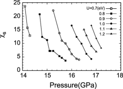
Figure 6: Pressure dependence of the maximum values of $\chi_{s}(\mbox{\boldmath{$q$}},\omega_{m}=0)$ for several values of $U$.

The result of this analysis is shown in Fig. 7, where the thickness of the lines represents the weight of the pairing determined from the value of $g(\delta)$. We can see that the direction in which the dominant pairings take place changes from $b$ to $b$$+$$c$ as the pressure increases, which looks more like $d_{xy}$-wave like pairing. These changes of the pairing directions are correlated with the increasing of hopping $t(p2)$. Thus, from the viewpoint of this real space analysis, we can say that the change of the dominant pairing direction due to the increase of $t(p2)$ suppress the tendency of the nesting vector $Q$ bridging the portions of Fermi surface with the same gap sign.

4.4 Origin of the “high $T_{c}$”

Finally, we discuss the reason why the obtained results, namely the values of $T_{c}$ and the form of the gap function, resemble that of the dimer limit approach. The present situation is in sharp contrast with the case of $\kappa$-(BEDT-TTF)₂X, where it has been known that, compared to the results of the dimer limit approach, [14, 15, 16] the position of the gap nodes changes and the values of $T_{c}$, if any, is drastically reduced in the original four band model with moderate dimerization[8, 9].

A large difference between the present case and $\kappa$-(BEDT-TTF)₂X is the Fermi surface nesting. As mentioned previously, the quasi-one-dimensionality of the system gives good Fermi surface nesting with strong spin fluctuations, fixing the nesting vector and thus the pairing symmetry firmly, while in the case of $\kappa$-(BEDT-TTF)₂X, the Fermi surface has no good Fermi surface nesting.

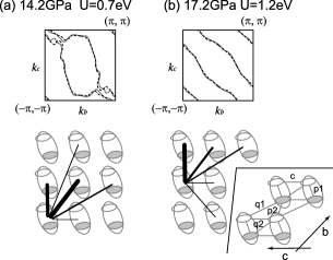
Figure 7: (upper panel) Results of the least squares fitting of the gap function. The dashed curve is the result of the FLEX calculation and the solid curve is the fitting. (lower panel) The weight of the directions in which the pairings take place for (a)$p=14.2$ GPa, $U=0.7$ eV (b) $p=17.2$ GPa, $U=1.2$ eV

However, it is unlikely that the good Fermi surface nesting alone can account for the resemblance between the 3/4-filled model and the dimer limit model because, for example, in the study for another organic superconductor (TMTSF)₂X, it has been known that a 1/4-filled model with no dimerization gives weak spin fluctuations within FLEX even though the Fermi surface nesting is very good.[17] One difference from the case of (TMTSF)${}_{2}X$ is the presence of moderate (not so weak) dimerization, but there is also a peculiar structure in the density of states as pointed out in the previous study.[4] Fig. 8(a) shows the density of states of the antibonding band at $p=17$ GPa for $U=0$. The two peaks near the Fermi level (energy=0) originates from the saddle points of the band dispersion located at the $\Gamma$ point and the Y point ($\mbox{\boldmath{$k$}}=(\pi,0)$). Consequently, the “Fermi surface with finite thickness”, defined by $E_{F}-\delta E<E(k_{x},k_{y})<E_{F}+\delta E$, becomes thick near the $\Gamma$ and the Y points, as shown in Fig. 8(b). In fact, this trend is already seen in the contour plots of the Green’s function in Figs. 3 and 5, where the bundles of the contour lines become thick near the $\Gamma$ and/or the Y points. Importantly, the wave vector (the nesting vector $\simeq(\pi,\pi/4)$) at which the spin fluctuations strongly develop bridges the states near the $\Gamma$ point and those somewhat close to the Y point (Fig. 8(b)), so that there are many states which contribute to the pair scattering. From the above argument, our results suggest that the coexistence of the good Fermi surface nesting, the large density of states near the Fermi level, and the moderate dimerization cooperatively enhances electron correlation effects, thereby giving results similar to those in the dimer (strong correlation) limit.

Now, these factors that enhance electron correlation should also make $T_{c}$ itself rather high. In fact, $T_{c}$ of $\sim 0.0006W$ almost reached in the present model, where $W$ is the band width (around $1.3$ eV for $p=16$ GPa), is relatively high among $T_{c}$ obtained by FLEX+Eliashberg equation approach in various Hubbard-type models. Namely, Arita et al. have previously shown[18] that $T_{c}$ of order $0.001W$ is about the highest we can reach within the Hubbard model[19], which is realized on a two dimensional square lattice near half filling, namely, a model for the high $T_{c}$ cuprates. The present study is in fact reminiscent of the FLEX study of the high $T_{c}$ cuprates, where the 3/4-filled two band model[20] and the half-filled single band model indeed give similar results on the superconducting $T_{c}$ and the pairing symmetry.[3] The cuprates also have a large density of states at the Fermi level originating from the so called hot spots around $(\pi,0)$ and $(0,\pi)$, and the wave vector $\sim(\pi,\pi)$ at which the spin fluctuations develop bridges these hot spots, as shown in Fig. 8(c). Moreover, a moderate band gap also exists in the cuprates between the fully filled bonding/non-bonding bands and the nearly half-filled antibonding band. The situation is thus somewhat similar to the present case. To conclude this section, it is highly likely that the coexistence of the factors that enhance correlation effects and thus make the results between the 3/4-filled original model and the half-filled dimer model similar is the very reason for the “high $T_{c}$” in the title material.

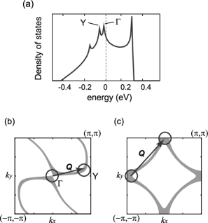
Figure 8: (a) The density of states of the antibonding band at $p=17$ GPa for $U=0$. (b) The Fermi surface with finite thickness defined by $E_{F}-\delta E<E(k_{x},k_{y})<E_{F}+\delta E_{F}$, where $E(k_{x},k_{y})$ is the band dispersion, and $\delta E_{F}=0.015$ eV is taken here. (c) A similar plot for the cuprates.

5 Conclusion

In the present paper, we have studied the pressure dependence of the superconducting transition temperature of an organic superconductor $\beta^{\prime}$-(BEDT-TTF)₂ICl₂ by applying two-band version of FLEX to the original two-band Hubbard model at $3/4$-filling with the hopping parameters determined from first principles calculation. The good Fermi surface nesting, the large density of states, and the moderate dimerization cooperatively enhance electron correlation effects, thereby leading to results similar to those in the dimer limit. We conclude that these factors that enhance electron correlation is the origin of the high $T_{c}$ in the title material.

As for the discrepancy between the present result and the experiment concerning the pressure regime where the superconducting phase appears, one reason may be due to the fact that we obtain $T_{c}$ only when $U\chi_{0}>0.995$ is not satisfied despite the fact that this criterion for “antiferromagnetic ordering”, originally adopted in the dimer model approach,[4] does not have a strict quantitative basis. Therefore, it may be possible to adopt, for example, $U\chi_{0}>0.999$ as a criterion for “antiferromagnetic ordering”, which will extend the superconducting phase into the lower pressure regime. Nevertheless, it seems that such consideration alone cannot account for the discrepancy because in order to “wipe out” the superconductivity in the high pressure regime as in the experiments, smaller values of $U$ would be necessary, which would give unrealistically low values of $T_{c}$. Another possibility for the origin of the discrepancy may be due to the ambiguity in determining the hopping integrals from first principles calculation. Further qualitative discussion may be necessary on this point in the future study.

References

- [1] T. Ishiguro, K. Yamaji and G. Saito: Organic superconductors (Springer-Verlag, Berlin, 1997) 2nd ed.
- [2] H. Taniguchi, M. Miyashita, K. Uchiyama, K. Satoh, N. Môri, H. Okamoto, K. Miyagawa, K. Kanoda, M. Hedo, and Y. Uwatoko J. Phys. Soc. Jpn. 72 (2003) L486.
- [3] N. E. Bickers, D. J. Scalapino, and S. R. White, Phys. Rev. Lett. 62 (1989) 961.
- [4] H. Kino, H. Kontani, and T. Miyazaki, J. Phys. Soc. Jpn. 73 (2004) L25.
- [5] H. Kontani, Phys. Rev. B 67 (2003) 180503(R).
- [6] T. Miyazaki and H. Kino, Phys. Rev. B 68 (2003) 225011(R).
- [7] H. Kino and H. Fukuyama, J. Phys. Soc. Jpn. 65 (1996) 2158.
- [8] H. Kondo and T. Moriya: J. Phys.: Condens. Matter 11 (1999) L363.
- [9] K. Kuroki, T. Kimura, R. Arita, Y. Tanaka ,and Y. Matsuda , Phys. Rev. B 65 (2002) 100516(R).
- [10] T. Komatsu, N. Matsukawa, T. Inoue, and G. Saito, J. Phys. Soc. Jpn. 65, 1340 (1996).
- [11] N. D. Mermin and H. Wagner, Phys. Rev. Lett. 17 (1966) 133
- [12] J.J. Deisz, D.W. Hess, and J.W. Serene, Phys. Rev. Lett. 76 (1996) 1312.
- [13] In previous studies, the Néel temperature is determined by a condition similar to eq.(10). In the present study, we do not evaluate because the antiferromagnetic phase in the actual material occurs below the Mott transition temperature (or the antiferromagnetic phase is within the Mott insulating phase), while a Mott transition cannot be treated within the present approach.
- [14] H. Kondo and T. Moriya, J. Phys. Soc. Jpn. 70 (2001) 2800.
- [15] J. Schmalian, Phys. Rev. Lett. 81 (1998) 4232.
- [16] H. Kino and H. Kontani, J. Phys. Soc. Jpn 67 (1998) L3691.
- [17] H. Kino and H. Kontani, J. Phys. Soc. Jpn. 68 (1999) 1481.
- [18] R. Arita, K. Kuroki, and H. Aoki, Phys. Rev. B. 60 (1999) 14585.
- [19] There are some exceptions which give extremely high within this approach, which is given, e.g. in, K. Kuroki and R. Arita 64 (2001) 024501.
- [20] S. Koikegami, S. Fujimoto, and K. Yamada, J. Phys. Soc. Jpn. 66 (1997) 1438.