Non-equilibrium Green’s function formalism and the problem of bound states

Abstract

The non-equilibrium Green’s function formalism for infinitely extended reservoirs coupled to a finite system can be derived by solving the equations of motion for a tight-binding Hamiltonian. While this approach gives the correct density for the continuum states, we find that it does not lead, in the absence of any additional mechanisms for equilibration, to a unique expression for the density matrix of any bound states which may be present. Introducing some auxiliary reservoirs which are very weakly coupled to the system leads to a density matrix which is unique in the equilibrium situation, but which depends on the details of the auxiliary reservoirs in the non-equilibrium case.

I Introduction

Electronic transport in mesoscopic systems has been studied intensively for several years datta ; imry ; landauer . For one-dimensional systems, the Landauer-Büttiker formalism has played a pivotal role in this subject landauer . For a wire in which only one channel is available to the electrons and the transport is ballistic (i.e., there are no impurities inside the wire, and there is no scattering from phonons or from the contacts between the wire and the reservoirs at its two ends), the zero-temperature conductance is given by $C_{0}=2e^{2}/h$ for infinitesimal bias. If there are impurities inside the wire which scatter the electrons, then the conductance is reduced from $C_{0}$.

A powerful calculational method for studying electronic transport is the non-equilibrium Green’s function (NEGF) formalism datta . The advantage of this method is that it treats the infinitely extended reservoirs (leads) in an exact way. The derivation of this formalism has been based on the Keldysh techniques keldysh ; caroli ; datta2 ; meir1 ; kamenev ; tsukada . Recently a simple derivation of the NEGF results based on a direct solution of the equations of motion for a non-interacting system of electrons was given in Ref. dhar, . This method, based on writing quantum Langevin equations, was first applied in the case of oscillator systems by Ford, Kac and Mazur fkm . It has recently been applied in the context of transport connell ; hanggi ; zurch ; segal ; ingold .

In the present paper we point out a particular problem that arises while using the NEGF formalism in a situation where there are bound states and there are no additional mechanisms for equilibration (such as electron-phonon scattering). We define bound states as states whose wave functions decay exponentially as one goes deep into any of the reservoirs. Their energy levels lie outside the energy band of all the reservoirs. One expects that the NEGF results should reduce to the usual equilibrium results if all the reservoirs are kept at the same chemical potential and temperature. This is easily shown to be true in the absence of bound states. In the presence of bound states, we show that while the contribution of the bound states to the equilibrium density matrix can be obtained within NEGF, the procedure is subtle and somewhat ad hoc. It is not clear in this formalism what the mechanism for equilibration of the bound states is. Moreover, if bound states are present, the density matrix is not unique in the non-equilibrium case. Here we show that the equation of motion approach can be used to obtain a clearer understanding of this problem of equilibration of bound states and the non-uniqueness of the non-equilibrium steady state. The central results of this paper are as follows.

(1) We give a simple and general derivation of the NEGF results by the equation of motion method for a system without interactions. This is obtained in two different ways: (i) from the steady state solution of the equations of motion, and (ii) from the general solution involving initial conditions.

(2) We show that, in the presence of bound states, the exact solution of the wire plus reservoir equations of motion (without any additional sources of equilibration) leads to steady states which depend on the initial conditions of the wire.

(3) We show that introducing additional broad-band auxiliary reservoirs (which are very weakly coupled to the wire) solves the problem of initial condition dependence. We obtain the non-equilibrium steady state properties in the limit where the coupling strength of the auxiliary reservoirs goes to zero. We find that the equilibrium density matrix is then unique and independent of the properties of the auxiliary reservoirs. But the non-equilibrium density matrix depends on the details of the auxiliary reservoirs and on the way in which their couplings (to the wire) are taken to zero.

Bound states have recently been studied in the context of the NEGF formalism wang1 ; wang2 , but to our knowledge, this particular problem of equilibration has not been addressed earlier. In this paper, we deal with electronic transport in non-interacting systems modeled by tight-binding Hamiltonians. For simplicity, we only consider spinless fermions here although it is quite straightforward to include spin.

The paper is organized as follows. In Sec. II, we discuss the NEGF formalism and present the expressions for the density matrix in the wire and the current. In Sec. III, we present a derivation of the NEGF results using the equation of motion method. This derivation is similar to that of Ref. dhar, but is a simplified and more generalized version. Starting from the full Heisenberg equations of motion of the wire and reservoirs, we derive effective quantum Langevin equations for the wire. These equations are solved by Fourier transforms to give the steady state solution which leads to expressions for the density matrix and the current which are identical to the results obtained from NEGF. In Sec. IV, we point out the problem of equilibration of bound states. In Sec. V, we consider the general solution of the equations of motion, as opposed to the steady state solution obtained in Sec. III. This lets us understand better the problem of equilibration in the presence of bound states. The question of the approach to the steady state (both in cases with or without bound states) can also be addressed in this approach. In Sec. VI, we describe our method of resolving the problem of equilibration of bound states. Namely, we introduce auxiliary reservoirs which are weakly coupled to the wire in such a way that the bound states which were earlier localized near the wire now extend infinitely into these new reservoirs, and the original bound state energy levels now lie within the energy band of the auxiliary reservoirs. The steady state properties are obtained in the limit in which the coupling of auxiliary reservoirs to the wire is taken to zero. In Sec.VII, we present some numerical results, for a system of a wire with a few sites coupled to one-dimensional reservoirs, to illustrate some of the analytical results. In Sec. VIII, we briefly consider systems of interacting electrons, and explain why a proper treatment of bound states is important for computing the current. In Sec. IX, we make some concluding remarks.

II Non-equilibrium Green’s function formalism

In this section, we will briefly discuss the NEGF formalism datta ; caroli ; datta2 ; meir1 ; tsukada ; dhar for a system which consists of a wire connected to reservoirs which are maintained at different chemical potentials or different temperatures. In the NEGF formalism, both the wire and the reservoirs are modeled by microscopic Hamiltonians. We will use a tight-binding model of non-interacting electrons which we will now describe. We use the following notation. For lattice sites anywhere on the system we will use the indices $r,s$; for sites on the wire ($W$) we will use the integer indices $i,j,k,\cdots$; for sites on the left reservoir ($L$) we use the Greek indices $\alpha,\nu$; finally, for sites on the right reservoir ($R$) we use the primed Greek indices $\alpha^{\prime},\nu^{\prime}$. We consider the following Hamiltonian of the full system:

$${\mathcal{H}} = \sum_{rs}~{}H_{rs}~{}c^{\dagger}_{r}c_{s}$$

$$= {\mathcal{H}}_{W}~{}+~{}{\mathcal{H}}_{L}~{}+~{}{\mathcal{H}}_{R}~{}+~{}{\mathcal{V}}_{L}~{}+~{}{\mathcal{V}}_{R}~{},$$

$${\rm where}\quad{\mathcal{H}}_{W} = \sum_{lm}~{}H^{W}_{lm}~{}c_{l}^{\dagger}c_{m}~{},~{}~{}~{}{{\mathcal{H}}}_{L}~{}=~{}\sum_{\alpha\nu}~{}H^{L}_{\alpha\nu}~{}c_{\alpha}^{\dagger}c_{\nu}~{},~{}~{}~{}{{\mathcal{H}}}_{R}~{}=~{}\sum_{\alpha^{\prime}\nu^{\prime}}~{}H^{R}_{\alpha^{\prime}\nu^{\prime}}~{}c_{\alpha^{\prime}}^{\dagger}c_{\nu^{\prime}}~{},$$

$${\mathcal{V}}_{L} = \sum_{l\alpha}~{}[~{}V^{L}_{l\alpha}~{}c_{l}^{\dagger}c_{\alpha}~{}+~{}{V^{L}_{\alpha l}}^{\dagger}~{}c_{\alpha}^{\dagger}c_{l}~{}]~{},$$

$${\mathcal{V}}_{R} = \sum_{l\alpha^{\prime}}~{}[~{}V^{R}_{l\alpha^{\prime}}~{}c_{l}^{\dagger}c_{\alpha^{\prime}}~{}+~{}{{V^{R}_{\alpha^{\prime}l}}^{\dagger}}~{}c_{\alpha^{\prime}}^{\dagger}c_{l}~{}]~{},$$

where $c_{r}^{\dagger},~{}c_{r}$ denote creation and destruction operators satisfying the usual fermionic anticommutation relations. The parts ${\mathcal{H}}_{W}$, ${\mathcal{H}}_{L}$ and ${\mathcal{H}}_{R}$ denote the Hamiltonians of the isolated wire, left and right reservoirs respectively, while $\mathcal{V}_{L}$ and $\mathcal{V}_{R}$ describe the coupling of the left and right reservoirs to the wire. The main results of NEGF are expressions for the steady state current and density matrix in the non-equilibrium steady state. To state these results we need a few definitions which we now make. Let $G^{+}(\omega)$ be the full single particle Green’s function of the system but defined between sites on the wire only. (See App. A for definitions of the various Green’s functions that will be used). Thus if the wire has $N$ sites then $G^{+}$ is a $N\times N$ matrix. It can be shown (see App. A) that $G^{+}$ is given by

$$G^{+}(\omega)=\frac{1}{\omega-H^{W}-\Sigma_{L}^{+}(\omega)-\Sigma_{R}^{+}(\omega)}~{},$$ (2)

where $\Sigma^{+}_{L,R}$ are self-energy terms which basically model the effect of the infinite reservoirs on the isolated wire Hamiltonian. (We will work in units in which Planck’s constant $\hbar=1$). The effective wire Hamiltonian is thus $H^{W}+\Sigma^{+}_{L}+\Sigma^{+}_{R}$ which in general will be shown to be non-Hermitian. The self energies can be written in terms of the isolated reservoir Green’s functions $g^{+}_{L,R}(\omega)$ and the coupling matrices $V^{L,R}$ (App. A). We get

$$\Sigma^{+}_{L}(\omega)=V^{L}~{}g^{+}_{L}(\omega)~{}{V^{L}}^{\dagger}~{},~{}~{}~{}~{}\Sigma^{+}_{R}(\omega)=V^{R}~{}g^{+}_{R}(\omega)~{}{V^{R}}^{\dagger}~{}.$$ (3)

Finally, let us use the following notation for the imaginary parts of the self energies from the two reservoirs,

$$\Gamma_{L}(\omega)=\frac{1}{2\pi i}[~{}\Sigma^{-}_{L}-\Sigma^{+}_{L}~{}]=V^{L}~{}\rho_{L}~{}{V^{L}}^{\dagger}~{},~{}~{}~{}~{}\Gamma_{R}(\omega)=\frac{1}{2\pi i}[~{}\Sigma^{-}_{R}-\Sigma^{+}_{R}~{}]=V^{R}~{}\rho_{R}~{}{V^{R}}^{\dagger}~{},$$ (4)

where $\Sigma^{-}(\omega)=Vg^{-}(\omega)V^{\dagger}$, and $\rho(\omega)=-(1/\pi)Im[g^{+}(\omega)]$ is the density matrix of an isolated reservoir.

With these definitions, NEGF gives the following expressions for the density matrix and current:

$$n_{lm} = \langle~{}c_{m}^{\dagger}(t)c_{l}(t)~{}\rangle$$

$$= \int_{-\infty}^{\infty}d\omega~{}[~{}(G^{+}\Gamma_{L}G^{-})_{lm}f(\omega,\mu_{L},T_{L})~{}+~{}(G^{+}\Gamma_{R}G^{-})_{lm}f(\omega,\mu_{R},T_{R})~{}]~{},$$

$$J = \sum_{m\alpha}~{}\langle~{}i~{}[~{}V_{m\alpha}^{*}~{}c^{\dagger}_{\alpha}(t)c_{m}(t)-V_{m\alpha}~{}c_{m}^{\dagger}(t)c_{\alpha}(t)~{}]~{}\rangle$$ (5)

$$= 2\pi\int_{-\infty}^{\infty}d\omega~{}Tr[~{}\Gamma_{L}G^{+}\Gamma_{R}G^{-}~{}]~{}(f(\omega,\mu_{L},T_{L})~{}-~{}f(\omega,\mu_{R},T_{R}))~{},$$

where $f(\omega,\mu,T)=1/[e^{\beta(\omega-\mu)}+1]$ denotes the Fermi function.

III Derivation of NEGF by “equation of motion approach”: Quantum Langevin equations and solution by Fourier transforms

In this section we give a derivation of the NEGF results using the equation of motion approach which was developed in Ref. dhar, . The derivation we present here is a simplified and generalized version of Ref. dhar, . This method basically involves writing the full equations of motion of the system of wire and reservoirs. The reservoir degrees are eliminated to give effective Langevin equations for the wire alone. Finally the Langevin equations, which are linear for the case of a non-interacting system, are solved by Fourier transformations to obtain the steady state properties.

The Heisenberg equations of motion for sites on the wire are:

$$\dot{c_{l}}=-i~{}\sum_{m}~{}H^{W}_{lm}~{}c_{m}~{}-~{}i~{}\sum_{\alpha}~{}V^{L}_{l\alpha}~{}c_{\alpha}~{}-~{}i~{}\sum_{\alpha^{\prime}}~{}V^{R}_{l\alpha^{\prime}}~{}c_{\alpha^{\prime}}~{},$$ (6)

and for sites on the reservoirs are:

$$\dot{c}_{\alpha} = -i~{}\sum_{\nu}~{}H^{L}_{\alpha\nu}~{}c_{\nu}~{}-~{}i~{}\sum_{l}~{}V^{L^{\dagger}}_{\alpha l}~{}c_{l}~{},$$

$$\dot{c}_{\alpha^{\prime}} = -i~{}\sum_{\nu^{\prime}}~{}H^{R}_{\alpha^{\prime}\nu^{\prime}}~{}c_{\nu^{\prime}}~{}-~{}i~{}\sum_{l}~{}V^{R^{\dagger}}_{\alpha^{\prime}l}~{}c_{l}~{}.$$ (7)

We solve the reservoir equations by treating them as linear equations with the term containing $c_{l}$ giving the inhomogeneous part. Using the Green’s functions

$$g^{+}_{L}(t)=-i~{}e^{-itH^{L}}~{}\theta(t)=\frac{1}{2\pi}\int_{-\infty}^{\infty}d\omega~{}g^{+}_{L}(\omega)e^{-i\omega t}~{},$$

$$g^{+}_{R}(t)=-i~{}e^{-itH^{R}}~{}\theta(t)=\frac{1}{2\pi}\int_{-\infty}^{\infty}d\omega~{}g^{+}_{R}(\omega)e^{-i\omega t}~{},$$ (8)

we get the following solutions for the reservoir equations of motion Eq. (7) (for $t>t_{0}$):

$$c_{\alpha}(t) = i~{}\sum_{\nu}~{}[g^{+}_{L}(t-t_{0})]_{\alpha\nu}~{}c_{\nu}(t_{0})~{}+~{}\int_{t_{0}}^{t}dt^{\prime}~{}\sum_{\nu l}~{}[g^{+}_{L}(t-t^{\prime})]_{\alpha\nu}~{}V^{L^{\dagger}}_{\nu l}~{}c_{l}(t^{\prime})~{},$$ (9)

$$c_{\alpha^{\prime}}(t) = i~{}\sum_{\nu^{\prime}}~{}[g^{+}_{R}(t-t_{0})]_{\alpha^{\prime}\nu^{\prime}}~{}c_{\nu^{\prime}}(t_{0})~{}+~{}\int_{t_{0}}^{t}dt^{\prime}~{}\sum_{\nu^{\prime}l}[g^{+}_{R}(t-t^{\prime})]_{\alpha^{\prime}\nu^{\prime}}~{}V^{R^{\dagger}}_{\nu^{\prime}l}~{}c_{l}(t^{\prime})~{}.$$ (10)

Plugging these into the equations of motion for the wire Eq. (6), we get:

$$\dot{c_{l}} = -i~{}\sum_{m}~{}H^{W}_{lm}~{}c_{m}~{}-~{}i\eta_{l}^{L}~{}-~{}i\int_{t_{0}}^{t}dt^{\prime}~{}\sum_{\alpha\nu m}V^{L}_{l\alpha}~{}[g^{+}_{L}(t-t^{\prime})]_{\alpha\nu}~{}V^{L^{\dagger}}_{\nu m}~{}c_{m}(t^{\prime})$$ (11)

$$-i~{}\eta_{l}^{R}~{}-~{}i\int_{t_{0}}^{t}dt^{\prime}~{}\sum_{\alpha^{\prime}\nu^{\prime}m}~{}V^{R}_{l\alpha^{\prime}}~{}[g^{+}_{R}(t-t^{\prime})]_{\alpha^{\prime}\nu^{\prime}}~{}V^{R^{\dagger}}_{\nu^{\prime}m}~{}c_{m}(t^{\prime})~{},$$

$${\rm where}\quad\eta_{l}^{L} = i~{}\sum_{\alpha\nu}~{}V^{L}_{l\alpha}~{}[g_{L}^{+}(t-t_{0})]_{\alpha\nu}~{}c_{\nu}(t_{0})~{},~{}~{}~{}\eta_{l}^{R}~{}=~{}i~{}\sum_{\alpha^{\prime}\nu^{\prime}}~{}V^{R}_{l\alpha^{\prime}}~{}[g_{R}^{+}(t-t_{0})]_{\alpha^{\prime}\nu^{\prime}}~{}c_{\nu^{\prime}}(t_{0})~{}.$$

We have broken up the reservoir contributions into noise and dissipative parts; it is clear that the wire equations now have the structure of quantum Langevin equations. The properties of the noise terms $\eta^{L},~{}\eta^{R}$ can be obtained from the condition that at time $t=t_{0}$, the two reservoirs are isolated and described by grand canonical ensembles at temperatures and chemical potentials given by $(T_{L},\mu_{L})$ and $(T_{R},\mu_{R})$ respectively. Thus we find, for the left reservoir,

$$\langle~{}{\eta_{l}^{L}}^{\dagger}(t)\eta_{m}^{L}(t^{\prime})~{}\rangle~{}=~{}\sum_{\alpha\nu\mu\sigma}~{}V^{L^{*}}_{l\alpha}~{}[{g_{L}^{+}}^{*}(t-t_{0})]_{\alpha\nu}~{}V^{L}_{m\mu}~{}[{g^{+}_{L}(t^{\prime}-t_{0})}]_{\mu\sigma}~{}\langle~{}c^{\dagger}_{\nu}(t_{0})c_{\sigma}(t_{0})~{}\rangle~{}.$$ (13)

Let $\psi^{L}_{q}(\alpha)$ and $\lambda^{L}_{q}$ denote the eigenvectors and eigenvalues of the left reservoir Hamiltonian $H^{L}$ which satisfy the equation

$$\sum_{m}~{}H^{L}_{\alpha\nu}~{}\psi^{L}_{q}(\nu)~{}=~{}\lambda^{L}_{q}~{}\psi^{L}_{q}(\alpha)~{}.$$ (14)

The equilibrium correlations are given by:

$$\langle c^{\dagger}_{\nu}(t_{0})c_{\sigma}(t_{0})\rangle=\sum_{q}\psi^{L^{*}}_{q}(\nu)~{}\psi^{L}_{q}(\sigma)~{}f(\lambda^{L}_{q},\mu_{L},T_{L})~{}.$$ (15)

Using this and the expansion $(g^{+}_{L})_{\nu\sigma}=-i\theta(t-t_{0})\sum_{q}\psi^{L}_{q}(\nu)~{}\psi_{q}^{L^{*}}(\sigma)~{}e^{-i\lambda^{L}_{q}(t-t_{0})}$ in Eq. (13), we get

$$\langle~{}{\eta^{L}}^{\dagger}_{l}(t)\eta_{m}^{L}(t^{\prime})~{}\rangle~{}=~{}\sum_{\alpha\nu}~{}V^{L^{*}}_{l\alpha}~{}[~{}\sum_{q}~{}\psi^{L^{*}}_{q}(\alpha)\psi^{L}_{q}(\nu)~{}e^{i\lambda^{L}_{q}(t-t^{\prime})}~{}f(\lambda^{L}_{q},\mu_{L},T_{L})~{}]~{}V^{L^{T}}_{\nu m}~{},$$ (16)

with similar results for the noise from the right reservoir. Now let us take the limits of infinite reservoir sizes and let $t_{0}\to-\infty$. On taking the Fourier transforms

$$\tilde{c}(\omega)=\frac{1}{2\pi}\int_{-\infty}^{\infty}dt~{}c(t)~{}e^{i\omega t}~{},~{}~{}~{}~{}\tilde{\eta}(\omega)=\frac{1}{2\pi}\int_{-\infty}^{\infty}dt~{}\eta(t)~{}e^{i\omega t}~{},$$ (17)

we get from Eq. (11):

$$\sum_{m}~{}[\omega\delta_{lm}-H^{W}_{lm}]~{}\tilde{c}_{m}(\omega) = \sum_{m}~{}(~{}[{\Sigma^{+}_{L}(\omega)}]_{lm}+[{\Sigma^{+}_{R}(\omega)}]_{lm}~{})~{}\tilde{c}_{m}(\omega)+\tilde{\eta}_{l}^{L}(\omega)+\tilde{\eta}^{R}_{l}(\omega)~{},$$

$${\rm{where}}~{}~{}~{}~{}\Sigma^{+}_{L} = V^{L}g^{+}_{L}{V^{L}}^{\dagger}~{},~{}~{}~{}~{}\Sigma^{+}_{R}=V^{R}g^{+}_{R}{V^{R}}^{\dagger}~{}.$$

The terms $\Sigma^{+}_{L},~{}\Sigma^{+}_{R}$ are the same self energies that appear in the NEGF formalism and effectively change the Hamiltonian, $H^{W}$, of the isolated wire, to $H^{W}+\Sigma^{+}_{L}(\omega)+\Sigma^{+}_{R}(\omega)$. The noise correlations can be obtained from Eq. (16) and give:

$$\langle~{}\tilde{\eta}_{l}^{L^{\dagger}}(\omega)\tilde{\eta}_{m}^{L}(\omega^{\prime})~{}\rangle = (V^{L}\rho^{L}{V^{L}}^{\dagger})_{ml}~{}f(\omega,\mu_{L},T_{L})~{}\delta(\omega-\omega^{\prime})$$ (19)

$$= \Gamma^{L}_{ml}(\omega)~{}f(\omega,\mu_{L},T_{L})~{}\delta(\omega-\omega^{\prime})~{},$$

$${\rm{where}}~{}~{}~{}\rho^{L}_{\alpha\nu}(\omega) = \sum_{q}\psi^{L}_{\alpha}(q)~{}\psi_{\nu}^{L^{*}}(q)~{}\delta(\omega-\lambda^{L}_{q})~{},$$

and similarly for the right reservoir. This is a fluctuation-dissipation relation and shows how the noise-noise correlations are related to the imaginary part of the self energy. Finally, we get the following steady state solutions of the equation of motion:

$$c_{l}(t) = \int_{-\infty}^{\infty}~{}d\omega~{}\tilde{c}_{l}(\omega)~{}e^{-i\omega t}~{},$$ (20)

$${\rm with}\quad\tilde{c}_{l}(\omega) = \sum_{m}~{}{G^{+}}_{lm}(\omega)~{}[~{}\tilde{\eta}^{L}_{m}(\omega)+\tilde{\eta}^{R}_{m}(\omega)~{}]~{},$$ (21)

$${\rm and}\quad G^{+}(\omega) = \frac{1}{\omega-H^{W}-\Sigma^{+}_{L}-\Sigma^{+}_{R}}~{}.$$ (22)

For the reservoir variables, we have from Eqs. (9,10)

$$\sum_{\alpha}~{}V^{L}_{l\alpha}~{}c_{\alpha}(\omega)=\tilde{\eta}^{L}_{l}(\omega)+\sum_{mn}[{\Sigma^{+}_{L}(\omega)}]_{lm}~{}G^{+}_{mn}(\omega)~{}[~{}\tilde{\eta}^{L}_{n}(\omega)+\tilde{\eta}^{R}_{n}(\omega)~{}]~{},$$ (23)

$$\sum_{\alpha^{\prime}}~{}V^{R}_{l\alpha^{\prime}}~{}c_{\alpha^{\prime}}(\omega)=\tilde{\eta}^{R}_{l}(\omega)+\sum_{mn}[{\Sigma^{+}_{R}(\omega)}]_{lm}~{}G^{+}_{mn}(\omega)~{}[~{}\tilde{\eta}^{L}_{n}(\omega)+\tilde{\eta}^{R}_{n}(\omega)~{}]~{}.$$ (24)

III.0.1 Steady state current and densities

Current: From a continuity equation, it is easy to see that the net current in the system is given by the following expectation value,

$$J=\sum_{m\alpha}\langle~{}i~{}[~{}V_{m\alpha}^{L^{*}}~{}c^{\dagger}_{\alpha}(t)~{}c_{m}(t)-V^{L}_{m\alpha}~{}c_{m}^{\dagger}(t)~{}c_{\alpha}(t)~{}]~{}\rangle=\sum_{m\alpha}2~{}Im[~{}V^{L}_{m\alpha}~{}\langle~{}c_{m}^{\dagger}(t)~{}c_{\alpha}(t)~{}\rangle~{}].$$ (25)

From the steady state solution (Eqs. 20-24), we get

$$\sum_{m\alpha}V^{L}_{m\alpha}~{}\langle c^{\dagger}_{m}(t)~{}c_{\alpha}(t)\rangle=\sum_{m\alpha}V^{L}_{m\alpha}~{}\int_{-\infty}^{\infty}d\omega~{}\int_{\infty}^{\infty}d\omega^{\prime}~{}e^{i(\omega-\omega^{\prime})t}~{}\langle~{}\tilde{c}^{\dagger}_{m}(\omega)~{}\tilde{c}_{\alpha}(\omega^{\prime})~{}\rangle$$

$$=\sum_{m}~{}\int_{-\infty}^{\infty}d\omega~{}\int_{\infty}^{\infty}d\omega^{\prime}~{}e^{i(\omega-\omega^{\prime})t}~{}\sum_{l}~{}\langle~{}G^{-}_{lm}(\omega)~{}[~{}\tilde{\eta}_{l}^{L^{\dagger}}(\omega)+\tilde{\eta}^{R^{\dagger}}_{l}(\omega)~{}]$$

$$~{}~{}~{}~{}~{}~{}~{}~{}~{}~{}~{}~{}~{}~{}~{}~{}~{}~{}~{}\times~{}[\tilde{\eta}_{m}^{L}(\omega^{\prime})+\sum_{jk}~{}[~{}{\Sigma^{+}_{L}(\omega^{\prime})}]_{mj}~{}G^{+}_{jk}(\omega^{\prime})~{}(~{}\tilde{\eta}^{L}_{k}(\omega^{\prime})+\tilde{\eta}^{R}_{k}(\omega^{\prime})~{})~{}]~{}\rangle~{}.$$ (26)

Let us consider that part of the above expression which depends only on the temperature and chemical potential of the right reservoir. This is given by

$$\int_{-\infty}^{\infty}d\omega~{}\int_{-\infty}^{\infty}d\omega^{\prime}~{}e^{i(\omega-\omega^{\prime})t}~{}\sum_{lmjk}~{}G^{-}_{lm}(\omega)~{}[{\Sigma^{+}_{L}(\omega^{\prime})}]_{mj}~{}G^{+}_{jk}(\omega^{\prime})~{}\langle~{}\tilde{\eta}^{R^{\dagger}}_{l}(\omega)~{}\tilde{\eta}^{R}_{k}(\omega^{\prime}))~{}\rangle$$

$$=\int_{-\infty}^{\infty}d\omega~{}\sum_{lmjk}~{}G^{-}_{lm}(\omega)[{\Sigma^{+}_{L}(\omega)}]_{mj}~{}G^{+}_{jk}(\omega)~{}{[\Gamma_{R}(\omega)]}_{kl}~{}f(\omega,\mu_{R},T_{R})~{}$$

$$=\int_{-\infty}^{\infty}d\omega~{}Tr[G^{-}(\omega)~{}\Sigma_{L}^{+}(\omega)~{}G^{+}(\omega)~{}\Gamma_{R}(\omega)]~{}f(\omega,\mu_{R},T_{R})~{}.$$

Taking the imaginary part of this and using this in Eq. (25), we find the contribution of the right reservoir to the current to be

$$J_{R}=-2\pi\int_{-\infty}^{\infty}d\omega~{}Tr[\Gamma_{L}G^{+}\Gamma_{R}G^{-}]~{}f(\omega,\mu_{R},T_{R})~{}.$$ (27)

[In deriving this result we used the identities $G^{+^{\dagger}}=G^{-},~{}\Sigma^{+^{\dagger}}=\Sigma^{-},~{}\Gamma^{\dagger}=\Gamma$ and the fact that $(Tr[M])^{*}=Tr[M^{\dagger}]$ for any matrix $M$]. It is clear that on adding the contribution of the left reservoir, we will get the net current (left-to-right) to be

$$J=2\pi\int_{-\infty}^{\infty}d\omega~{}Tr[\Gamma_{L}G^{+}\Gamma_{R}G^{-}]~{}(f(\omega,\mu_{L},T_{L})-f(\omega,\mu_{R},T_{R}))~{}.$$ (28)

Densities: The density matrix is given by the expression

$$n_{lm} = \langle~{}c_{m}^{\dagger}(t)~{}c_{l}(t)~{}\rangle$$ (29)

$$= \int_{-\infty}^{\infty}d\omega\int_{-\infty}^{\infty}d\omega^{\prime}~{}e^{i(\omega-\omega^{\prime})t}~{}\sum_{kj}~{}G_{km}^{-}(\omega)~{}\langle~{}[\tilde{\eta}_{k}^{L^{\dagger}}(\omega)+\tilde{\eta}_{k}^{R^{\dagger}}(\omega)]~{}[\tilde{\eta}^{L}_{j}(\omega^{\prime})+\tilde{\eta}^{R}_{j}(\omega^{\prime})]~{}\rangle~{}G^{+}_{lj}(\omega^{\prime})$$

$$= \int_{-\infty}^{\infty}d\omega~{}[~{}(G^{+}\Gamma_{L}G^{-})_{lm}~{}f(\omega,\mu_{L},T_{L})+(G^{+}\Gamma_{R}G^{-})_{lm}~{}f(\omega,\mu_{R},T_{R})~{}]~{}.$$

The results in Eq. (28,29) are identical to the results from NEGF given in Sec. II. For $\mu_{L}=\mu_{R}$ and $T_{L}=T_{R}$, we get the expected equilibrium value [see App. (B)] provided that there are no bound states.

IV Problems with bound states

A desirable property of the NEGF results is that they should reduce to the standard equilibrium results for the case when both reservoirs are at the same chemical potential and temperatures, i.e., for $\mu_{L}=\mu_{R}=\mu$ and $T_{L}=T_{R}=T$. For this case the current vanishes, which is the correct result expected from equilibrium. For the density, we get from Eq. (5):

$$n_{lm} = \int_{-\infty}^{\infty}d\omega~{}[G^{+}(\omega)~{}(~{}\Gamma_{L}(\omega)+\Gamma_{R}(\omega)~{})~{}G^{-}(\omega)]_{lm}~{}f(\omega,\mu,T)~{},$$ (30)

$${\rm with}~{}~{}~{}~{}G^{+}(\omega) = \frac{1}{\omega-H^{W}-\Sigma^{+}_{L}(\omega)-\Sigma^{+}_{R}(\omega)}~{}.$$ (31)

The expected equilibrium result can be obtained using the grand canonical ensemble, and we get (see App. B):

$$n^{eq}_{lm} = \int_{-\infty}^{\infty}d\omega~{}[G^{+}~{}(\Gamma_{L}+\Gamma_{R})~{}G^{-}]_{lm}~{}f(\omega,\mu,T)~{}+~{}\int_{-\infty}^{\infty}d\omega~{}\frac{\epsilon}{\pi}~{}[G^{+}G^{-}]_{lm}~{}f(\omega,\mu,T)~{},~{}~{}~{}~{}~{}~{}~{}$$ (33)

$${\rm where}~{}~{}G^{+}(\omega)=\frac{1}{\omega+i\epsilon-H^{W}-\Sigma^{+}_{L}(\omega)-\Sigma^{+}_{R}(\omega)}~{}.$$

Note that here we retain the $i\epsilon$ factor in the Green’s function. The $i\epsilon$ factor in Eq. (31) can be dropped since, for $\omega$ in the range of interest in Eq. (30), the self energies $\Sigma^{+}_{L}$ and $\Sigma^{+}_{R}$ have finite imaginary parts. (Whenever we introduce $\epsilon$ in an equation, it is understood that it is an infinitesimal positive quantity which has to be taken to zero at the end of the calculation). The first piece in Eq. (33) is identical to the NEGF prediction, while it can be shown that the second piece vanishes only if there are no bound states. Thus in the absence of bound states we verify that the NEGF results reduce to the correct equilibrium results.

Let us discuss now the case when there are bound states. Here we refer to bound states of the full system of wire and reservoirs. The bound states have energies lying outside the range of the reservoir levels, and the wave functions corresponding to them decay exponentially as one goes deep into the reservoirs. They are obtained as real solutions of the equation

$$[H^{W}+\Sigma^{+}_{L}(\lambda_{b})+\Sigma^{+}_{R}(\lambda_{b})]~{}\Psi_{b}~{}=~{}\lambda_{b}\Psi_{b}~{}.$$ (34)

From the form of the Green’s function, it is clear that the second term in Eq. (33) is non-vanishing whenever the above equation has real $\lambda_{b}$ solutions, and it can be shown to reduce to the form

$$n^{eq-bnd}_{lm}~{}=~{}\sum_{b}~{}\Psi_{b}(l)\Psi^{*}_{b}(m)~{}f(\lambda_{b},\mu,T)~{}.$$ (35)

Thus there seems to be a problem of equilibration in the NEGF formalism whenever bound states are present. This problem can be fixed in the following way. In the NEGF results let us add an extra infinitesimal part $\epsilon_{a}/\pi$ to the matrix $\Gamma_{a}(\omega)$ corresponding to the $a^{\rm th}$ reservoir ($a=L,~{}R$). Thus the NEGF result for the density matrix is modified to

$$n_{lm}~{}=~{}\langle c_{m}^{\dagger}(t)c_{l}(t)\rangle = \int_{-\infty}^{\infty}d\omega~{}[~{}(G^{+}\Gamma_{L}G^{-})_{lm}~{}f(\omega,\mu_{L},T_{L})+(G^{+}\Gamma_{R}G^{-})_{lm}~{}f(\omega,\mu_{R},T_{R})~{}]$$

$$+ \int_{-\infty}^{\infty}d\omega~{}[~{}\frac{\epsilon_{L}}{\pi}~{}(G^{+}G^{-})_{lm}~{}f(\omega,\mu_{L},T_{L})+\frac{\epsilon_{R}}{\pi}~{}(G^{+}G^{-})_{lm}~{}f(\omega,\mu_{R},T_{R})~{}],$$

$${\rm with}~{}~{}~{}G^{+}(\omega) = \frac{1}{\omega-H^{W}-\Sigma^{+}_{L}(\omega)-\Sigma^{+}_{R}(\omega)+i(\epsilon_{L}+\epsilon_{R})}~{}.$$ (36)

The second integral gets contributions from bound states. Using the identity

$$\lim_{{\epsilon_{L,R}}\to 0}~{}\frac{\epsilon_{a}}{(\omega-\lambda_{b})^{2}+(\epsilon_{L}+\epsilon_{R})^{2}}~{}=~{}\lim_{{\epsilon_{L,R}}\to 0}~{}\pi\frac{\epsilon_{a}}{\epsilon_{L}+\epsilon_{R}}\delta(\omega-\lambda_{b})~{},$$ (37)

we finally get the following contribution from the bound states,

$$n^{bnd}_{lm}=\sum_{b}~{}\lim_{{\epsilon_{L,R}}\to 0}~{}\frac{\epsilon_{L}f(\lambda_{b},\mu_{L},T_{L})+\epsilon_{R}f(\lambda_{b},\mu_{R},T_{R})}{\epsilon_{L}+\epsilon_{R}}~{}\Psi_{b}(l)\Psi_{b}^{*}(m)~{}.$$ (38)

For $\mu_{L}=\mu_{R}=\mu$ and $T_{L}=T_{R}=T$, we now get the expected equilibrium result of Eq. (35). For the non-equilibrium case, however, the situation is somewhat unsatisfactory since the density matrix depends on the ratio $\epsilon_{L}/\epsilon_{R}$, and so the bound state contribution is ambiguous. More importantly, in this approach it is not at all clear as to what the exact physical mechanism for equilibration of the bound states is.

In the following sections, we will examine this particular question of equilibration of bound states more carefully.

V General solution of equations of motion

In this section, we will consider the general solution of the equations of motion. Unlike the Fourier transform solution obtained in Sec. III, the general solution also involves the initial conditions of the wire. The advantage of the equations of motion method is that it can address issues such as that of approach to the steady state, it can be numerically implemented (after truncating the reservoirs to a finite number of sites), and it does not rely on any ad hoc $i\epsilon$ prescriptions for the reservoirs. We will show that the expression for the density matrix can be derived without any difficulties if there are no bound states. Further, the problems which arise if there is a bound state become quite clear in this approach.

Let us again consider a system in which a wire is connected to two reservoirs, with

$${\mathcal{H}}~{}=~{}\sum_{r,s}~{}H_{rs}~{}c_{r}^{\dagger}~{}c_{s}~{}.$$ (39)

As before we will use the label $r,s$ to denote any site in the system, and $j$, $\alpha$ and $\alpha^{\prime}$ to denote sites in the wire and left and right reservoirs respectively. Instead of eliminating the reservoir degrees of motion and writing Langevin equations for the wire, we will now deal with the full Heisenberg equations of motion for the system which is given by

$$\dot{c}_{r}~{}=~{}-i~{}\sum_{s}~{}H_{rs}~{}c_{s}~{}.$$ (40)

At the initial time $t=0$, we assume that the two reservoirs are in thermal equilibrium at temperatures and chemical potentials $T_{L,R}$ and $\mu_{L,R}$, and the couplings $V^{L,R}$ are zero. As before, let $\lambda^{a}_{q}$ and $\psi^{a}_{q}$, with $a=L,R$, denote the eigenvalues and eigenfunctions of the isolated reservoir Hamiltonians. At $t=0$, the density matrix for sites on the left and right reservoirs are given respectively by

$$\langle c^{\dagger}_{\alpha}(0)c_{\nu}(0)\rangle = \sum_{q}~{}\psi^{L^{*}}_{q}(\alpha)\psi^{L}_{q}(\nu)~{}f(\lambda^{L}_{q},\mu_{L},T_{L})~{},$$

$$\langle c^{\dagger}_{\alpha^{\prime}}(0)c_{\nu^{\prime}}(0)\rangle = \sum_{q}~{}\psi^{R^{*}}_{q}(\alpha^{\prime})\psi^{R}_{q}(\nu^{\prime})~{}f(\lambda^{R}_{q},\mu_{R},T_{R})~{}.$$ (41)

We also assume that at $t=0$, there are no correlations between the two reservoirs and between the wire and the reservoirs. Thus

$$\langle~{}c^{\dagger}_{l}(0)~{}c_{\alpha}(0)~{}\rangle~{}=~{}\langle~{}c^{\dagger}_{l}(0)~{}c_{\alpha^{\prime}}(0)~{}\rangle~{}=~{}\langle~{}c^{\dagger}_{\alpha}(0)~{}c_{\alpha^{\prime}}(0)~{}\rangle~{}=~{}0~{}.$$ (42)

Finally, for sites in the wire, we cannot unambiguously assign a value to the density matrix $\langle c_{l}^{\dagger}(0)c_{m}(0)\rangle$ at $t=0$, since the wire is isolated from everything else at that time. Under certain conditions, we will see that in the steady state (defined as the limit $t\to\infty$), the density matrix of the wire will turn out to be independent of its value at $t=0$.

Let us now suddenly switch on the couplings $V_{a}$ of the wire to the reservoirs at $t=0$. For $t>0$, the solution of the equations of motion is given in matrix notation by

$$c(t)~{}=~{}i~{}{\mathcal{G}}^{+}(t)~{}c(0)~{},$$ (43)

where ${\mathcal{G}}^{+}(t)=-ie^{-iHt}\theta(t)$, and $c(t)=[c_{1},~{}c_{2}...,~{}c_{N_{s}}]^{T}$, where $N_{s}$ is the total number of sites in entire system. For a point $l$ in the wire, we then have

$$c_{l}(t)~{}=~{}\sum_{m}~{}{\mathcal{G}}^{+}_{lm}(t)~{}c_{m}(0)~{}+~{}\sum_{\nu}~{}{\mathcal{G}}^{+}_{l\nu}~{}c_{\nu}(0)~{}+~{}\sum_{\nu^{\prime}}~{}{\mathcal{G}}^{+}_{l\nu^{\prime}}~{}c_{\nu^{\prime}}(0)~{}.$$ (44)

Hence the density matrix in the wire is given by

$$n_{lm}(t) = \langle c^{\dagger}_{m}(t)c_{l}(t)\rangle$$ (45)

$$= ~{}\sum_{ij}~{}{\mathcal{G}}^{+}_{lj}(t)~{}\langle c^{\dagger}_{i}(0)c_{j}(0)\rangle~{}{\mathcal{G}}^{-}_{im}(t)~{}+~{}\sum_{\alpha\nu}~{}{\mathcal{G}}^{+}_{l\alpha}(t)~{}\langle c^{\dagger}_{\nu}(0)c_{\alpha}(0)\rangle~{}{\mathcal{G}}^{-}_{\nu m}(t)$$

$$~{}+~{}\sum_{\alpha^{\prime}\nu^{\prime}}~{}{\mathcal{G}}^{+}_{l\alpha^{\prime}}(t)~{}\langle c^{\dagger}_{\nu^{\prime}}(0)c_{\alpha^{\prime}}(0)\rangle~{}{\mathcal{G}}^{-}_{\nu^{\prime}m}(t)~{}.$$

Now let $\Psi_{Q}(r)$ and $\lambda_{Q}$ denote the eigenfunctions and eigenvalues respectively of the system of coupled wire and reservoirs. Thus

$$\sum_{s}~{}H_{rs}~{}\Psi_{Q}(s)~{}=~{}\lambda_{Q}\Psi_{Q}(r)~{}.$$ (46)

Then the full Green’s function can be written in the following way (for $t>0$):

$${\mathcal{G}}^{+}_{rs}(t) = -i~{}\sum_{Q}~{}\Psi_{Q}(r)\Psi^{*}_{Q}(s)~{}e^{-i\lambda_{Q}t}$$ (47)

$$= -i~{}\sum_{b}~{}\Psi_{b}(r)\Psi^{*}_{b}(s)~{}e^{-i\lambda_{b}t}~{}-~{}i~{}\int d\omega~{}\rho^{c}_{rs}(\omega)~{}e^{-i\omega t}~{},$$

where $\Psi_{b},~{}\lambda_{b}$ refer to bound states, and the density matrix $\rho^{c}$ is given by a sum over the extended (continuum) states of the system $\rho^{c}_{rs}(\omega)=\sum_{Q}^{c}\Psi_{Q}(r)\Psi_{Q}^{*}(s)\delta(\omega-\lambda_{Q})$. In the limit $t\to\infty$, the second term vanishes (this follows from the Riemann-Lebesgue lemma, see Ref. bender, ), and we get a contribution only from bound states. Thus

$$\lim_{t\to\infty}{\mathcal{G}}^{+}_{rs}(t)~{}=~{}-i~{}\sum_{b}~{}\Psi_{b}(r)\Psi^{*}_{b}(s)~{}e^{-i\lambda_{b}t}~{}.$$ (48)

Thus if there are no bound states in the fully coupled system then, for any two sites of the system, ${\mathcal{G}}^{+}_{rs}(t)$ vanishes as $t\to\infty$. From this it follows that the contribution of any finite number of terms in Eq. (45) vanishes in the steady state. Since the wire consists of a finite number of sites, this means that the initial density matrix of the wire $\langle c^{\dagger}_{i}(0)c_{j}(0)\rangle$ will have no effect on the steady state density matrix $n_{lm}(t\to\infty)$. The reason that Eq. (45) does not vanish in the steady state is that it gets contributions from the reservoirs which have an infinite number of sites. On the other hand the situation is quite different if there are one or more bound states in the problem. In that case, clearly, individual matrix elements of ${\mathcal{G}}^{+}$ may not vanish in the steady state, and the initial state of the wire makes a contribution to the long time density matrix.

We now look at the contribution of the reservoirs in Eq. (45). Dropping the subscript $a$ for the moment, let us look at the contribution of any one of the reservoirs. Using Eq. (41), this can be written as

$$n^{res}_{lm}(t) = \sum_{\alpha\nu}~{}\int_{-\infty}^{\infty}~{}{d\omega}~{}f(\omega,\mu,T)~{}{\mathcal{G}}^{+}_{l\alpha}(t)~{}\sum_{q}~{}\psi_{q}(\alpha)\psi^{*}_{q}(\nu)~{}\delta(\omega-\lambda_{q})~{}{\mathcal{G}}^{-}_{\nu m}(t)$$ (49)

$$\equiv \int_{-\infty}^{\infty}{d\omega}~{}f(\omega,\mu,T)~{}I_{lm}(\omega,t)~{},$$

$${\rm where}~{}~{}~{}I_{lm}(\omega,t) = \sum_{\alpha\nu}{\mathcal{G}}^{+}_{l\alpha}(t)~{}[~{}\sum_{q}~{}\psi_{q}(\alpha)\psi^{*}_{q}(\nu)~{}\delta(\omega-\lambda_{q})~{}]~{}{\mathcal{G}}^{-}_{\nu m}(t)~{}.$$

We now transform to the frequency dependent Green’s function using the relation ${\mathcal{G}}^{+}(t)~{}=~{}\int_{-\infty}^{\infty}\frac{d\omega}{2\pi}{\mathcal{G}}^{+}(\omega)e^{-i\omega t}$. As shown in App. A, we can express the Green’s function elements ${\mathcal{G}}^{+}_{j\nu}(\omega)$ in terms of $G^{+}_{ij}(\omega)$ and the isolated reservoir Green’s functions $g^{+}_{\alpha\nu}(\omega)$. We get

$${\mathcal{G}}^{+}_{l\alpha}(\omega) = \sum_{j\nu}~{}G^{+}_{lj}(\omega)~{}V_{j\nu}~{}g^{+}_{\nu\alpha}(\omega)~{},$$

$${\rm and}\quad{\mathcal{G}}^{-}_{\alpha l}(\omega) = \sum_{j\nu}~{}g^{-}_{\alpha\nu}(\omega)~{}V^{\dagger}_{\nu j}~{}G^{-}_{jl}(\omega)~{}.$$ (50)

We will also use the following result which follows from an eigenfunction expansion of $g^{+}(\omega)$,

$$\sum_{\alpha}~{}g^{+}_{\nu\alpha}(\omega)\psi_{q}(\alpha)~{}=~{}\sum_{\alpha}~{}[\sum_{q^{\prime}}\frac{\psi_{q^{\prime}}(\nu)\psi^{*}_{q^{\prime}}(\alpha)}{\omega+i\epsilon-\lambda_{q^{\prime}}}]~{}\psi_{q}(\alpha)~{}=~{}\frac{\psi_{q}(\nu)}{\omega+i\epsilon-\lambda_{q}}~{}.$$ (51)

Using Eqs. (50-51), we can write $I_{lm}(\omega,t)$ in Eq. (49) as

$$I_{lm}(\omega,t)$$ (52)

$$= \frac{1}{2\pi}\int d\omega^{\prime}~{}\sum_{j\nu\alpha i}~{}\frac{G^{+}_{lj}(\omega^{\prime})e^{-i\omega^{\prime}t}}{\omega^{\prime}+i\epsilon-\omega}V_{j\nu}~{}[~{}\sum_{q}\psi_{q}(\nu)\psi^{*}_{q}(\alpha)\delta(\omega-\lambda_{q})~{}]~{}V^{\dagger}_{\alpha i}~{}\frac{1}{2\pi}\int d\omega^{\prime\prime}\frac{G^{-}_{im}(\omega^{\prime\prime})e^{i\omega^{\prime\prime}t}}{\omega^{\prime\prime}-i\epsilon-\omega}$$

$$= \frac{1}{2\pi}\int d\omega^{\prime}~{}\sum_{ji}~{}\frac{G^{+}_{lj}(\omega^{\prime})e^{-i\omega^{\prime}t}}{\omega^{\prime}+i\epsilon-\omega}~{}[V\rho(\omega)V^{\dagger}]_{ji}~{}\frac{1}{2\pi}\int d\omega^{\prime\prime}~{}\frac{G^{-}_{im}(\omega^{\prime\prime})e^{i\omega^{\prime\prime}t}}{\omega^{\prime\prime}-i\epsilon-\omega}~{}.$$

The first integral in the above equation can be evaluated as follows:

$$\frac{1}{2\pi}\int d\omega^{\prime}\frac{G^{+}_{lj}(\omega^{\prime})e^{-i\omega^{\prime}t}}{\omega^{\prime}+i\epsilon-\omega} = \sum_{Q}~{}\Psi_{Q}(l)\Psi_{Q}^{*}(j)~{}\frac{1}{2\pi}\int_{-\infty}^{\infty}d\omega^{\prime}~{}\frac{e^{-i\omega^{\prime}t}}{(\omega^{\prime}+i\epsilon-\omega)(\omega^{\prime}+i\epsilon^{\prime}-\lambda_{Q})}$$ (53)

$$= -iG^{+}_{lj}(\omega)e^{-i\omega t}~{}+~{}i\sum_{Q}~{}\Psi_{Q}(l)\Psi_{Q}^{*}(j)~{}\frac{e^{-i\lambda_{Q}t}}{\omega+i\epsilon-\lambda_{Q}}~{}.$$

In the limit $t\to\infty$, only the bound states contribute to the summation (over $Q$) in the expression above. Hence we get

$$\lim_{t\to\infty}~{}\frac{1}{2\pi}\int d\omega^{\prime}~{}\frac{G^{+}_{lj}(\omega^{\prime})e^{-i\omega^{\prime}t}}{\omega^{\prime}+i\epsilon-\omega}=-i~{}G^{+}_{lj}(\omega)~{}e^{-i\omega t}+i~{}\sum_{b}~{}\Psi_{b}(l)\Psi_{b}^{*}(j)~{}\frac{e^{-i\lambda_{b}t}}{\omega-\lambda_{b}}~{}.$$ (54)

Note that we have dropped the $i\epsilon$ factor in the denominator of the second term. This is because of the following reason. In the expression Eq. (52), the presence of the density of states of the reservoirs $\rho(\omega)$ means that we will be interested only in values of $\omega$ lying in the continuum of reservoir eigenvalues. Using Eq. (54), we finally get the following result for the contribution from the $a^{\rm{th}}$ reservoir to the density matrix in the long time limit:

$$n^{a}_{lm} = \int_{-\infty}^{\infty}d\omega~{}[~{}G^{+}(\omega)\Gamma^{a}(\omega)G^{-}(\omega)~{}]_{lm}~{}f(\omega,\mu_{a},T_{a})$$

$$+~{}\sum_{bb^{\prime}}e^{-i(\lambda_{b}-\lambda_{b^{\prime}})t}~{}\sum_{ji}~{}\Psi_{b}(l)\Psi^{*}_{b}(j)\Psi_{b^{\prime}}(i)\Psi_{b^{\prime}}^{*}(m)~{}\int_{-\infty}^{\infty}d\omega~{}\frac{[~{}\Gamma_{a}(\omega)~{}]_{ji}~{}f(\omega,\mu_{a},T_{a})}{(\omega-\lambda_{b})(\omega-\lambda_{b^{\prime}})}~{},$$

where $b,b^{\prime}$ denote bound states, and we have again dropped terms in which the integrands contain time-dependent oscillatory factors.

In the absence of bound states, we see that the contribution of the reservoirs is identical to that given by NEGF and also by the Fourier-transform solution in Sec. III. However, in the presence of bound states, there is an extra contribution which is not obtained in the other methods. Importantly, this extra part is, in general, time-dependent so that the system never reaches a stationary state. Also, we do not recover the equilibrium results for the case when all reservoirs are kept at equal temperatures and chemical potentials. The reason for this is that the reservoirs are not able to equilibrate bound state energy levels since these levels lie outside the range of the reservoir band of energies.

VI A solution to the bound state problem

One way to solve the bound state equilibration problem is to introduce two auxiliary reservoirs $\bar{L}$ and $\bar{R}$; these must have the same temperature and chemical potentials as the original reservoirs $L$ and $R$, but they must have a large enough bandwidth so that any bound states of the original Hamiltonian ${\mathcal{H}}$ lie within that bandwidth. (Briefly, the idea is that since the bound states of ${\mathcal{H}}$ are no longer bound states in the expanded system, the arguments given in Sec. IV imply that the density matrix of the wire will no longer depend on the initial density matrix). The two auxiliary reservoirs must be coupled very weakly to the wire, so that they do not greatly alter the energies of ${\mathcal{H}}$ and the corresponding wave functions within the wire and the original reservoirs. We will eventually take the limit of that coupling going to zero. The main purpose of the auxiliary reservoirs is to equilibrate any bound states which ${\mathcal{H}}$ might have. Let us now see how all this works.

We consider a new Hamiltonian of the form

$${\mathcal{H}}_{\rm new} = {\mathcal{H}}~{}+~{}{\mathcal{H}}_{\bar{L}}~{}+~{}{\mathcal{H}}_{\bar{R}}~{}+~{}{\mathcal{V}}_{\bar{L}}~{}+~{}{\mathcal{V}}_{\bar{R}}~{},$$ (56)

$${\rm where}\quad{\mathcal{H}} = {\mathcal{H}}_{W}+{\mathcal{H}}_{L}+{\mathcal{H}}_{R}+{\mathcal{V}}_{L}+{\mathcal{V}}_{R}~{}.$$

${\mathcal{H}}_{\bar{a}}$ denotes the Hamiltonian of the auxiliary reservoirs (${\bar{a}}={\bar{L}},{\bar{R}}$), and ${\mathcal{V}}_{\bar{a}}$ denotes the coupling of those reservoirs to the wire. The auxiliary reservoirs will also be taken to be lattice systems with tight-binding Hamiltonians, but with a hopping amplitude which is sufficiently large. We will take the auxiliary reservoir $\bar{L}$ to have the same temperature and chemical potential $T_{L}$ and $\mu_{L}$ as the reservoir $L$, and similarly for the reservoirs $\bar{R}$ and $R$.

Following the derivation of Sec. III, we find that the full Green’s function on the wire is now given by

$${\bar{G}}^{+}(\omega)~{}=~{}\frac{1}{\omega~{}-~{}H^{W}~{}-~{}\Sigma^{+}_{L}(\omega)~{}-~{}\Sigma^{+}_{R}(\omega)~{}-~{}\Sigma^{+}_{\bar{L}}(\omega)~{}-~{}\Sigma^{+}_{\bar{R}}(\omega)}~{}.$$ (57)

With the auxiliary reservoirs present, there are no longer any bound states, and the density matrix in the wire can be written as

$$n_{lm}= \int_{-\infty}^{\infty}d\omega~{}[\bar{G}^{+}(\Gamma_{L}+\Gamma_{\bar{L}})\bar{G}^{-}]_{lm}~{}f(\omega,\mu_{L},T_{L})$$

$$+~{}\int_{-\infty}^{\infty}d\omega~{}[\bar{G}^{+}(\Gamma_{R}+\Gamma_{\bar{R}})\bar{G}^{-}]_{lm}f(\omega,\mu_{R},T_{R})~{}.$$

We want to eventually take the limit in which the couplings of the wire to the auxiliary reservoirs $V_{\bar{a}}$ go to zero. We will therefore treat these couplings perturbatively. Let us first break up the above integral over $\omega$ into two parts, one with $\omega$ going over the range of the original reservoir band, and the other containing the remaining part over the range of the auxiliary reservoir. We assume that the original reservoir bandwidths are in the range $[E_{1},E_{2}]$ while that of the auxiliary reservoirs are $[{\bar{E}}_{1},{\bar{E}}_{2}]$; we choose the latter such that it contains the original bandwidth, i.e., ${\bar{E}}_{1}<E_{1}$ and ${\bar{E}}_{2}>E_{2}$. Thus we write:

$$n_{lm} = n^{1}_{lm}+n^{2}_{lm}~{},$$

$$n^{1}_{lm} = \int_{E_{1}}^{E_{2}}d\omega~{}[\bar{G}^{+}(\Gamma_{L}+\Gamma_{\bar{L}})\bar{G}^{-}]_{lm}f(\omega,\mu_{L},T_{L})+\int_{E_{1}}^{E_{2}}d\omega~{}[\bar{G}^{+}(\Gamma_{R}+\Gamma_{\bar{R}})\bar{G}^{-}]_{lm}f(\omega,\mu_{R},T_{R}),$$

$$n^{2}_{lm} = \int_{\bar{E}_{1}}^{E_{1}}d\omega~{}[\bar{G}^{+}\Gamma_{\bar{L}}\bar{G}^{-}]_{lm}f(\omega,\mu_{L},T_{L})~{}+~{}\int_{\bar{E}_{1}}^{E_{1}}d\omega~{}[\bar{G}^{+}\Gamma_{\bar{R}}\bar{G}^{-}]_{lm}f(\omega,\mu_{R},T_{R})$$ (58)

$$+~{}\int_{E_{2}}^{\bar{E}_{2}}d\omega~{}[\bar{G}^{+}\Gamma_{\bar{L}}\bar{G}^{-}]_{lm}f(\omega,\mu_{L},T_{L})~{}+~{}\int_{E_{2}}^{\bar{E}_{2}}d\omega~{}[\bar{G}^{+}\Gamma_{\bar{R}}\bar{G}^{-}]_{lm}f(\omega,\mu_{R},T_{R})~{}.$$

Now, in the first part ($n^{1}$) we note that both $\Sigma^{+}_{L}$ and $\Sigma^{+}_{R}$ have finite imaginary parts. Hence on taking the limit $V_{{\bar{L}},{\bar{R}}}\to 0$, we immediately get $\Gamma_{{\bar{L}},{\bar{R}}}\to 0$ and $\bar{G}^{+}(\omega)=G^{+}(\omega)$. Hence

$$n^{1}_{lm}~{}=~{}\int_{E_{1}}^{E_{2}}d\omega~{}[G^{+}\Gamma_{L}G^{-}]_{lm}~{}f(\omega,\mu_{L},T_{L})~{}+~{}\int_{E_{1}}^{E_{2}}d\omega~{}[G^{+}\Gamma_{R}G^{-}]_{lm}~{}f(\omega,\mu_{R},T_{R})~{},$$ (59)

which is just the usual reservoir contribution.

We will now show that the second part contributes to bound states only. As before, let us denote the eigenvalues and eigenfunctions of the combined system of the wire and reservoirs (but not the auxiliary reservoirs) by $\lambda_{Q}$ and $\Psi_{Q}$, where the label $Q$ can have both a continuous and a discrete part (corresponding to bound states). We will assume that the auxiliary reservoirs have been chosen such that all the values of $\lambda_{Q}$ lie within the bandwidth of the auxiliary reservoirs. The coupling to the auxiliary reservoirs cause the energy levels to shift from $\lambda_{Q}$ to $\lambda_{Q}+\delta\lambda_{Q}$. To first order in $V_{\bar{a}}$, we find that

$$\delta\lambda_{Q}~{}=~{}\langle\Psi_{Q}|\Sigma^{+}_{\bar{L}}(\lambda_{Q})+\Sigma^{+}_{\bar{R}}(\lambda_{Q})|\Psi_{Q}\rangle~{}=~{}\sum_{jk}~{}\Psi^{*}_{Q}(j)~{}[\Sigma^{+}_{\bar{L}}+\Sigma^{+}_{\bar{R}}]_{jk}~{}\Psi_{Q}(k)~{}.$$ (60)

The imaginary part of $\delta\lambda_{Q}$ is therefore given by

$${\rm Im}~{}\delta\lambda_{Q}=-{\pi}\sum_{j,k}~{}\Psi^{*}_{Q}(j)~{}[\Gamma_{\bar{L}}+\Gamma_{\bar{R}}]_{j,k}~{}\Psi_{Q}(k)~{}.$$ (61)

Thus for the auxiliary reservoir $\bar{a}$ we get

$$\sum_{km}~{}\bar{G}^{+}_{jk}[\Gamma_{{\bar{a}}}]_{km}\bar{G}^{-}_{ml}~{}=~{}\sum_{km}~{}\sum_{Q}~{}\frac{\Psi_{Q}(j)\Psi^{*}_{Q}(k)}{\omega-\lambda_{Q}-\delta\lambda_{Q}}~{}[\Gamma_{\bar{a}}]_{km}~{}\sum_{Q^{\prime}}~{}\frac{\Psi_{Q^{\prime}}(m)\Psi^{*}_{Q^{\prime}}(l)}{\omega-\lambda_{Q^{\prime}}-\delta\lambda^{*}_{Q^{\prime}}}~{}.$$ (62)

Since we are considering values of $\omega$ outside the range $[E_{1},E_{2}]$, it is clear that, in the limit $\Gamma_{\bar{a}}\to 0$, only bound states with $\lambda_{Q}=\lambda_{Q^{\prime}}=\lambda_{b}$ will contribute. The above then gives

$$\lim_{\Gamma_{\bar{a}}\to 0}~{}\sum_{km}~{}\bar{G}^{+}_{jk}[\Gamma_{{\bar{a}}}]_{km}\bar{G}^{-}_{ml} = \sum_{km}~{}\sum_{b}~{}\frac{\Psi_{b}(j)\Psi^{*}_{b}(k)~{}[\Gamma_{{\bar{a}}}]_{km}~{}\Psi_{b}(m)\Psi^{*}_{b}(l)}{(\omega-\lambda_{b}-~{}{\rm Re}~{}\delta\lambda_{b})^{2}~{}+~{}({\rm Im}~{}\delta\lambda_{b})^{2}}$$ (63)

$$= \sum_{b}~{}\frac{\langle\Psi_{b}|\Gamma_{\bar{a}}|\Psi_{b}\rangle}{\langle\Psi_{b}|\Gamma_{\bar{L}}+\Gamma_{\bar{R}}|\Psi_{b}\rangle}~{}\delta(\omega-\lambda_{b})~{}\Psi_{b}(j)~{}\Psi^{*}_{b}(l)~{},$$

where we have used the fact that both real and imaginary parts of $\delta\lambda_{b}$ are small, with the imaginary part given by Eq. (61).

Putting everything together, we finally find that the total density matrix in the wire due to all four reservoirs is given by

$$n_{lm} = ~{}\int_{E_{1}}^{E_{2}}d\omega~{}[~{}(~{}G^{+}(\omega)\Gamma_{L}(\omega)G^{-}(\omega)~{})_{lm}~{}f_{L}(\omega)+(~{}G^{+}(\omega)\Gamma_{R}(\omega)G^{-}(\omega)~{})_{lm}~{}f_{R}(\omega)~{}]$$ (64)

$$+~{}\sum_{b}~{}\frac{\langle\Psi_{b}|\Gamma_{\bar{L}}|\Psi_{b}\rangle f_{L}(\lambda_{b})~{}+~{}\langle\Psi_{b}|\Gamma_{\bar{R}}|\Psi_{b}\rangle f_{R}(\lambda_{b})}{\langle\Psi_{b}|\Gamma_{\bar{L}}~{}+~{}\Gamma_{\bar{R}}|\Psi_{b}\rangle}~{}\Psi_{b}(l)\Psi^{*}_{b}(m)~{},$$

where the sum over $b$ runs over all the bound states of $H$. In the equilibrium case [i.e., for $f_{L}(\lambda_{b})=f_{R}(\lambda_{b})$] Eq. (64) shows that the contribution of a bound state $b$ to the density matrix is independent of details of the auxiliary reservoirs such as the quantities $\langle\Psi_{b}|\Gamma_{\bar{L}}|\Psi_{b}\rangle$ and $\langle\Psi_{b}|\Gamma_{\bar{R}}|\Psi_{b}\rangle$. But in the non-equilibrium case [i.e., for $f_{L}(\lambda_{b})\neq f_{R}(\lambda_{b})$], the contribution of a bound state does depend on details of the auxiliary reservoirs, namely, on the ratio $\langle\Psi_{b}|\Gamma_{\bar{L}}|\Psi_{b}\rangle/\langle\Psi_{b}|\Gamma_{\bar{R}}|\Psi_{b}\rangle$. This is perhaps not surprising. Some quantities in equilibrium statistical mechanics may be independent of the mechanism for equilibration, while the same quantities in non-equilibrium statistical mechanics may depend on the details of that mechanism.

The similarity between Eq. (38) and the bound state contribution in Eq. (64) implies that we can think of the auxiliary reservoirs as providing a justification for the $i\epsilon_{a}$ prescription which was introduced in the NEGF formalism in Sec. II.

We note that bound states do not carry current, and so the expressions for current remain unchanged. Later we will point out that in the presence of electron-electron interactions, even the current is likely to be affected by bound states.

VII Numerical results

It is instructive to consider the following simple examples where we can explicitly see the problem of equilibration of bound states and its resolution by the introduction of auxiliary reservoirs.

VII.1 Wire with a single site

We will first consider a system where the wire ($W$) consists of a single site with an on-site potential and connected to one reservoir ($R$) and one auxiliary reservoir (${\bar{R}}$). The reservoirs are one-dimensional semi-infinite electronic lattices. The full Hamiltonian is thus given by

$${\mathcal{H}} = {\mathcal{H}}_{W}+{\mathcal{H}}_{R}+{\mathcal{H}}_{\bar{R}}+{\mathcal{V}}_{R}+{\mathcal{V}}_{\bar{R}}~{},$$

$${\mathcal{H}}_{W} = Vc^{\dagger}_{0}c_{0}~{},$$

$${\mathcal{H}}_{R} = -\gamma~{}\sum_{\alpha=-\infty}^{-2}~{}(c_{\alpha}^{\dagger}c_{\alpha+1}+c_{\alpha+1}^{\dagger}c_{\alpha})~{},$$

$${\mathcal{V}}_{R} = -\gamma^{\prime}~{}(c_{-1}^{\dagger}c_{0}+c^{\dagger}_{0}c_{-1})~{},$$

$${\mathcal{H}}_{\bar{R}} = -{\bar{\gamma}}\sum_{\bar{\alpha}=-\infty}^{-2}(c_{\bar{\alpha}}^{\dagger}c_{\bar{\alpha}+1}+c_{\bar{\alpha}+1}^{\dagger}c_{\bar{\alpha}})~{},$$

$${\mathcal{V}}_{\bar{R}} = -{\bar{\gamma}}^{\prime}(c_{-\bar{1}}^{\dagger}c_{0}+c^{\dagger}_{0}c_{-\bar{1}})~{}.$$ (65)

Let us first give the exact equilibrium results for the system of wire and the single reservoir. The reservoir will be assumed to have a chemical potential $\mu$ and temperature $T$. From App. B, we get for the density at the single site on the wire

$$n^{eq} = n_{r}^{eq}+n_{b}^{eq}~{},$$

$$\rm{where}\quad n_{r}^{eq} = \int_{-2}^{2}d\omega~{}{\gamma^{\prime}}^{2}~{}|G_{00}^{+}(\omega)|^{2}~{}\rho(\omega)~{}f(\omega,\mu,T)~{},$$

$$n_{b}^{eq} = \int_{-\infty}^{\infty}d\omega~{}\frac{\epsilon}{\pi}~{}|G^{+}_{00}(\omega)|^{2}~{}f(\omega,\mu,T)~{},$$ (66)

$${\rm and}\quad G^{+}_{00}(\omega) = \frac{1}{\omega+i\epsilon-V-{\gamma^{\prime}}^{2}~{}g^{+}(\omega)}~{}.$$ (67)

We need $g^{+}(\omega)$ and $\rho(\omega)$ which are the reservoir Greens function and the reservoir density of states respectively, both evaluated at the site $\alpha=-1$. The eigenvalues and eigenfunctions of the reservoir Hamiltonian are given by

$$\lambda_{q}~{}=~{}-2~{}\gamma~{}\cos q~{},\quad{\rm and}\quad\psi_{q}(\alpha)~{}=~{}\sqrt{2}\sin(q~{}\alpha)~{},$$ (68)

where $q$ lies in the range $[0,\pi]$, and $n=-1,-2,\cdots$. The wave functions are normalized so that $\langle\psi_{q}|\psi_{q^{\prime}}\rangle=\pi\delta(q-q^{\prime})$. Hence we get for the required reservoir Green’s function,

$$g^{+}(\omega) = \frac{1}{\gamma}~{}[~{}\frac{\omega}{2}-i~{}(1-\frac{\omega^{2}}{4\gamma^{2}})^{1/2}~{}]\quad{\rm for}\quad|\omega|<2\gamma$$

$$= \frac{1}{\gamma}~{}[~{}\frac{\omega}{2}+(\frac{\omega^{2}}{4\gamma^{2}}-1)^{1/2}~{}]\quad{\rm for}\quad\omega<-2\gamma$$

$$= \frac{1}{\gamma}~{}[~{}\frac{\omega}{2}-(\frac{\omega^{2}}{4\gamma^{2}}-1)^{1/2}~{}]\quad{\rm for}\quad\omega>2\gamma~{},$$

$$\rho(\omega) = \frac{1}{\gamma\pi}(1-\frac{\omega^{2}}{4\gamma^{2}})^{1/2}\quad{\rm for}\quad|\omega|<2\gamma$$ (69)

$$= 0\quad{\rm for}\quad|\omega|>2\gamma~{}.$$

Similarly, for the auxiliary reservoir we get,

$$\bar{g}^{+}(\omega) = \frac{1}{{\bar{\gamma}}}[\frac{\omega}{2{\bar{\gamma}}}-i(1-\frac{\omega^{2}}{4{\bar{\gamma}}^{2}})^{1/2}]\quad{\rm for}\quad|\omega|<2{\bar{\gamma}}$$

$$= \frac{1}{{\bar{\gamma}}}[\frac{\omega}{2{\bar{\gamma}}}+(\frac{\omega^{2}}{4{\bar{\gamma}}^{2}}-1)^{1/2}]\quad{\rm for}\quad\omega<-2{\bar{\gamma}}$$

$$= \frac{1}{{\bar{\gamma}}}[\frac{\omega}{2{\bar{\gamma}}}-(\frac{\omega^{2}}{4{\bar{\gamma}}^{2}}-1)^{1/2}]\quad{\rm for}\quad\omega>2{\bar{\gamma}}~{},$$

$$\bar{\rho}(\omega) = \frac{1}{{\bar{\gamma}}\pi}(1-\frac{\omega^{2}}{4{\bar{\gamma}}^{2}})^{1/2}\quad{\rm for}\quad|\omega|<2{\bar{\gamma}}$$ (70)

$$= 0\quad{\rm for}\quad|\omega|>2{\bar{\gamma}}~{}.$$

Bound states: We choose the parameter values $\gamma=\gamma^{\prime}=1$. For the coupled system of wire and reservoir, we again get a continuum of states identical to the original reservoir levels. In addition, for $V<-1$, we get a bound state whose energy is given by $\lambda_{b}=V+1/V$, and the wave function at the $0^{th}$ site is $\Psi_{b}(0)=(1-1/V^{2})^{1/2}$.

System without auxiliary reservoir: In our numerical example we take $V=-2,~{}\mu=0$, and $\beta=2$. Thus, from Eq. (67), the expected equilibrium results are

$$n^{eq}_{r} = \int_{-2}^{2}d\omega~{}\frac{\rho(\omega)f(\omega,\mu,T)}{|\omega-V-g^{+}(\omega)|^{2}}~{}=~{}0.1641...~{},$$

$$n^{eq}_{b} = \Psi_{b}(0)^{2}f(\lambda_{b},\mu,T)~{}=~{}0.7449...~{},$$

$$n^{eq} = n^{eq}_{r}+n^{eq}_{b}~{}=~{}0.9091...~{}.$$ (71)

We have numerically solved the equations of motion for a reservoir with $L=500$ sites. In Fig. 1, we show the contribution of the reservoir to the density at the $0^{\rm{th}}$ site as a function of time by a solid line. We find that it quickly settles at a value of about $n^{R}=0.314$. The contribution coming from an initial density equal to one at site $0$, namely, $\lim_{t\to\infty}G^{+}_{00}(t)G^{-}_{00}(t)$ in Eq. (45), is shown by a dashed line. This does not vanish with time but settles at a value of about $n^{In}=0.563$. This means that the steady state density on the wire depends on the initial density. Using the results of Sec. V we can understand the different contributions to the density. From Eq. (48), we get the contribution from the initial density as

$$n^{In}~{}=~{}|\Psi_{b}(0)|^{4}~{}=~{}0.5625~{},$$ (72)

which is close to the numerically obtained result. From Eq. (LABEL:rescont), we see that there are two parts to the contribution from the reservoir levels. The first part is a contribution to the density at site $0$ arising from the extended states; this is identical to the equilibrium result $n_{ext}^{R}=n^{eq}_{r}=0.1641...$. The second part is from the bound state; from Eq. (LABEL:rescont) this is given by

$$n_{bnd}^{R}~{}=~{}|\Psi_{b}(0)|^{4}~{}\int_{-2}^{2}d\omega~{}\frac{\rho(\omega)}{(\omega-\lambda_{b})^{2}}~{}f(\omega,\mu,T)~{}=~{}0.1500...~{}.$$

Hence we get $n^{R}=n_{ext}^{R}+n_{bnd}^{R}=0.3141...$. We note in Fig. 1 that for large times which are of the order of the reservoir size, both the contributions start deviating from their steady values; we will comment more on this below.

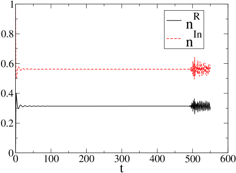
Figure 1: Time evolution of the contributions of a single reservoir ($n^{R}$) and the initial condition on the wire ($n^{In}$) to the density at that site, for $\gamma=\gamma^{\prime}=1$, $\beta=2$, $\mu=0$, and $V=-2$.

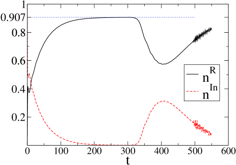
Figure 2: Time evolution of the contributions of the two reservoirs ($n^{R}$) and the initial conditions on wire ($n^{In}$) to the density at that site, for $\gamma=\gamma^{\prime}=1$, ${\bar{\gamma}}=2$, ${\bar{\gamma}^{\prime}}=0.2$, $\beta=2$, $\mu=0$, and $V=-2$.

System with auxiliary reservoir: We now introduce an auxiliary reservoir with the same temperature, chemical potential and number of sites as the original reservoir. However, we take the hopping amplitude in this reservoir to be ${\bar{\gamma}}=2$, so that its bandwidth of $[-4,4]$ includes the energy of the bound state of the original system. We take the coupling of the auxiliary reservoir to site 0 to be ${\bar{\gamma}^{\prime}}=0.2$. We now solve the equations of motion of this new system consisting of two reservoirs and one site. Fig. 2 shows the total contribution of the two reservoirs by a solid line, and the contribution coming from an initial density of one at site 1 by a dashed line. We see that the solid line approaches a value of $0.907$ (this deviates slightly from the equilibrium value of $0.909$ because $\bar{\gamma}^{\prime}$, though small, is not zero), while the dashed line vanishes around the same time. Using the results in Sec. VI, we can compute the contributions of the reservoir and the auxiliary reservoir to the net density. We get

$$n^{R}~{}=~{}\int_{-2}^{2}d\omega~{}\frac{\rho(\omega)f(\omega,\mu,T)}{|\omega-V-g^{+}(\omega)-{\bar{\gamma}}^{\prime 2}\bar{g}^{+}(\omega)|^{2}}~{}=~{}0.1614...~{},$$

$$n^{\bar{R}}~{}=~{}\int_{-4}^{4}d\omega~{}\frac{{\bar{\gamma}}^{\prime 2}\bar{\rho}(\omega)f(\omega,\mu,T)}{|\omega-V-g^{+}(\omega)-{\bar{\gamma}}^{\prime 2}\bar{g}^{+}(\omega)|^{2}}~{}=~{}0.7458...~{}.$$ (73)

Hence the total density is $n=n^{R}+n^{\bar{R}}=0.9072...$ which is consistent with the value obtained from the numerics. Comparing with Eq. (71) we note that the auxiliary reservoir only contributes to equilibration of the bound state.

In Fig. 3, we show an example where the potential $V=-0.5$ is such that there are no bound states. In this case we find, as expected, that the wire equilibrates even with a single reservoir. Adding an auxiliary reservoir leaves the density essentially unchanged.

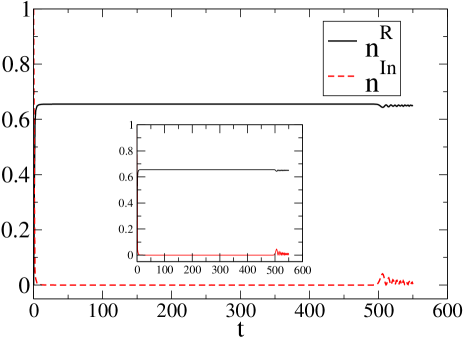
Figure 3: Time evolution of the contributions of a single reservoir ($n^{R}$) and the initial conditions on wire ($n^{In}$) to the density at that site, for $\gamma=\gamma^{\prime}=1$, $\beta=2$, $\mu=0$, and $V=-0.5$. The inset shows the time evolution for the case with two reservoirs.

The time scale of approaching these steady values is of the order of $\tau={\bar{\gamma}}/{\bar{\gamma}}^{{}^{\prime}2}=50$. This is due to the fact that the self-energy of the auxiliary reservoir is proportional to ${\bar{\gamma}}^{{}^{\prime}2}/{\bar{\gamma}}$. This governs the rate at which the auxiliary reservoir fills up site 1, and it is inversely proportional to $\tau$. For times $t>>\tau$, we obtain the correct equilibrium value of the density at site 0 (up to a small error due to the finiteness of $\bar{\gamma}^{\prime}$). Further, the vanishing of the dashed line means that the steady state density at site 0 does not depend on the initial density at that site. Once again, we see in Fig. 2 that for large times of the order of the reservoir sizes, both the contributions start deviating from their steady values.

The deviations which begin appearing in Figs. 1-3 at large times of the order of the reservoir sizes can be understood as follows. After the wire is suddenly connected to one end of a reservoir at time $t=0$, there is a recurrence time of the reservoir which is given by the time it takes for the effect of that connection to propagate to the other end of the reservoir, and then return to the wire. If the reservoir has a size $L$, and the Fermi velocity in the reservoir is $v_{F}$ (this is equal to $2\gamma\sin k_{F}$ and $2{\bar{\gamma}}\sin k_{F}$ for the original and auxiliary reservoirs respectively), the recurrence time is given by $2L/v_{F}$. Since we have taken $\mu=0$ (half-filling), we have $k_{F}=\pi/2$, and $v_{F}=L/\gamma$ and $L/{\bar{\gamma}}$ in the two reservoirs respectively. In Figs. 1-3, we see deviations occurring at a time given by $L=500$ due to the original reservoir, while in Fig. 2, we also see deviations occurring at a time equal to $L/{\bar{\gamma}}=250$ due to the auxiliary reservoir.

The presence of the recurrence times imply that one must take the limits of certain quantities going to infinity in a particular order, in order to numerically obtain the correct steady state values of the density matrix. The coupling $\bar{\gamma}^{\prime}$ of the auxiliary reservoirs to the wire must be taken to zero so that the steady state values do not depend on the details of those reservoirs (at least in the equilibrium case); this means that $\tau$ must go to infinity. On the other hand, the recurrence time $2L/v_{F}$ must also go to infinity. The steady state will then exist for times $t$ which satisfy $\tau<<t<<2L/v_{F}$.

Approach to equilibrium: Let us briefly discuss the way in which equilibrium is approached at times which are small compared to the recurrence times discussed above. One again, there are two different time scales here, one for the original reservoirs and the other for the auxiliary reservoirs (if there is a bound state present). For the original reservoirs, let us consider an integral of the form given in the second term in Eq. (47), namely, $\int_{E_{1}}^{E_{2}}d\omega~{}\rho(\omega)e^{-i\omega t}$, where the function $\rho(\omega)$ has no singularities in the range $[E_{1},E_{2}]$. Let us also suppose that $\rho(\omega)$ has the power-law forms $(\omega-E_{1})^{\alpha_{1}}$ and $(E_{2}-\omega)^{\alpha_{2}}$ at the two ends of the integral, where $\alpha_{1},~{}\alpha_{2}>-1$ so that the integral exists. Then one can use the method of steepest descent to show that in the limit $t\to\infty$, the above integral only gets a contribution from the end points, and those contributions vanish as $e^{-iE_{1}t}/t^{\alpha_{1}+1}$ and $e^{-iE_{2}t}/t^{\alpha_{2}+1}$ respectively bender . For the original reservoirs with $\gamma=\gamma^{\prime}=1$, this approach to equilibrium occurs at times of the order $1/\gamma$, and it is therefore hard to see the power-law fall-off in Figs. 1 and 4. For the auxiliary reservoirs, the time scale of equilibration is given by a different expression if there is a bound state present. The relevant integral is then given by $\int_{{\bar{E}}_{1}}^{{\bar{E}}_{2}}d\omega~{}\rho(\omega)e^{-i\omega t}$, where the function $\rho(\omega)$ is large in the vicinity of the bound state energy $\lambda_{b}$, namely, $\rho(\omega)\sim({\bar{\gamma}}^{{}^{\prime}2}/{\bar{\gamma}})/[(\omega-\lambda_{b})^{2}+({\bar{\gamma}}^{{}^{\prime}2}/{\bar{\gamma}})^{2}]$ where ${\bar{\gamma}}/{\bar{\gamma}}^{{}^{\prime}2}$ is large. We then see that the dominant contribution to the integral comes from the vicinity of $\omega=\lambda_{b}$ and is given by $e^{-t~{}{\bar{\gamma}}^{{}^{\prime}2}/{\bar{\gamma}}}$. We can see this exponential decay in Fig. 2, till the effect of the shortest recurrence times starts becoming visible.

VII.2 Wire with two sites

In the presence of two bound states, the steady state properties can be time dependent. We now illustrate this with the example of a two-site wire. We take both sites (labeled 0 and 1) to have an on-site potential $V=-3$. The site 0 is connected to a one-dimensional semi-infinite reservoir (going from $-1$ to $-L$ as in the previous example), while site 1 is only coupled to site 0. The Green’s function is thus

$$G^{+}(\omega)=\left(\begin{array}[]{cc}\omega-V-g^{+}(\omega)&1\cr 1&\omega-V\end{array}\right)^{-1}$$ (76)

Let us look at the density at site $0$ in the long time limit. From the equation of motion solution in Sec. V, we expect the density to have contributions from both the initial density matrix on the wire ($n^{In}$) and from the reservoir ($n^{R}$). We choose the initial wire density matrix to be diagonal, with $\langle c^{\dagger}_{0}c_{0}\rangle=1$. Then from Eq. (47) we get

$$n^{In}~{}=~{}|\Psi_{b_{1}}(0)|^{4}~{}+~{}|\Psi_{b_{2}}(0)|^{4}~{}+~{}2~{}|\Psi_{b_{1}}(0)|^{2}|\Psi_{b_{2}}(0)|^{2}~{}\cos{(\lambda_{b_{1}}-\lambda_{b_{2}})t}~{}.$$ (77)

The contribution from the reservoirs consists of two parts: one corresponding to the extended states $n^{R}_{ext}$, and the other to the bound states $n^{R}_{bnd}$. These are given by

$$n^{R}_{ext} = \int_{-2}^{2}d\omega~{}|G^{+}_{00}|^{2}~{}\rho(\omega)~{}f(\omega,\mu,T)$$

$$n^{R}_{bnd} = |\Psi_{b_{1}}(0)|^{4}~{}\int_{-2}^{2}d\omega~{}\frac{\rho(\omega)f(\omega,\mu,T)}{(\omega-\lambda_{b_{1}})^{2}}~{}+~{}|\Psi_{b_{2}}(0)|^{4}~{}\int_{-2}^{2}d\omega~{}\frac{\rho(\omega)f(\omega,\mu,T)}{(\omega-\lambda_{b_{2}})^{2}}~{},$$ (78)

$$+~{}2~{}|\Psi_{b_{1}}(0)|^{2}|\Psi_{b_{2}}(0)|^{2}~{}\cos{(\lambda_{b_{1}}-\lambda_{b_{2}})t}~{}\int_{-2}^{2}d\omega~{}\frac{\rho(\omega)f(\omega,\mu,T)}{(\omega-\lambda_{b_{1}})(\omega-\lambda_{b_{2}})}~{}.$$

The bound state eigenvalues are obtained by solving, for $\omega=-2\cosh{\alpha}<0$, the equation

$$Det~{}[\left(\begin{array}[]{cc}\omega-v-g^{+}(\omega)&1\cr 1&\omega-v\end{array}\right)]~{}=~{}0~{}.$$ (81)

With $g^{+}(\omega)=-e^{-\alpha}$ this gives the equation

$$e^{3\alpha}+2ve^{2\alpha}+v^{2}e^{\alpha}+v~{}=~{}0~{},$$

which, for $V=-3$, has two solutions with $\alpha>0$. These give the eigenvalues $\lambda_{b_{1}}=-2.257...$ and $\lambda_{b_{2}}=-4.137...$. The eigenvectors can also be found easily after normalizing them over the entire system. At site 0, we get

$$|\Psi_{b}(0)|^{2}~{}=~{}\frac{(1-e^{-2\alpha})(v+2\cosh{\alpha})^{2}}{(1-e^{-2\alpha})+(v+2\cosh{\alpha})^{2}}~{}.$$

This gives $|\Psi_{b_{1}}|^{2}=0.2947...$ and $|\Psi_{b_{2}}|^{2}=0.5421...$. Then from Eq. (77) and Eq. (78) we get

$$n^{In} = 0.381~{}+~{}0.3196~{}\cos(1.879t)~{},$$

$$n^{R}_{ext} = 0.1097~{},$$

$$n^{R}_{bnd} = 0.05654~{}+~{}0.045~{}\cos(1.879t)~{}.$$ (82)

We verify these results by an exact numerical solution of the time evolution of the system with the two-site wire and a one-dimensional reservoir with $L=600$ sites. In Fig. 4, we compare the analytic results with the numerical solution and find very good agreement between the two. The inset shows the long time behavior; we see that the effect of the finite size of the reservoir shows up at the recurrence time $2L/v_{F}=600$. In Fig. 5, we show the effect of adding a weakly coupled (${\bar{\gamma}}^{\prime}=0.3$) auxiliary reservoir with ${\bar{\gamma}}=3$. As expected, in this case there is no contribution from the initial density of the wire, and the reservoir contribution gives the equilibrium value (till the effect of the recurrence time of the auxiliary reservoir, $L/{\bar{\gamma}}=200$, shows up).

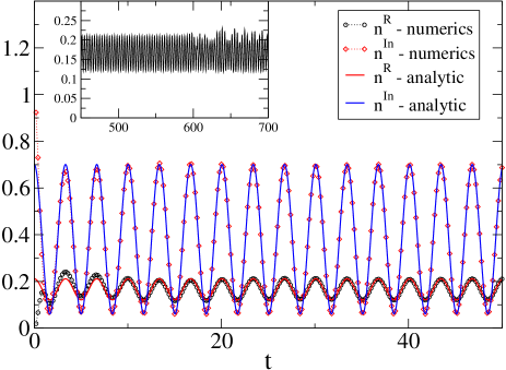
Figure 4: Time evolution of the contributions of the reservoir ($n^{R}$) and initial conditions on wire ($n^{In}$) to the density at the first site of a two-site system, for $\gamma=\gamma^{\prime}=1$, $\beta=2,~{}\mu=0$ and $v=-3$. The analytic predictions are also plotted.

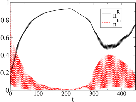
Figure 5: Time evolution of the contributions of the two reservoirs ($n^{R}$) and the initial density on site ($n^{In}$) to the density at the first site of a two-site system, for $\gamma=\gamma^{\prime}=1$, ${\bar{\gamma}}=3$, ${\bar{\gamma}^{\prime}}=0.3$, $\beta=2$, $\mu=0$, and $V=-3$.

VIII Interacting systems

Let us briefly consider how interactions can be studied within the NEGF formalism. We note that this formalism works with a one-particle Hamiltonian, e.g., the self-energy in Eq. (2) is given in terms of the energy of a single electron which is entering or leaving the wire. One way to deal with interactions is therefore to do a Hartree-Fock (HF) decomposition. For instance, if we have a Hubbard model with an on-site interaction between spin-up and spin-down electrons of the form $Uc_{n\uparrow}^{\dagger}c_{n\uparrow}c_{n\downarrow}^{\dagger}c_{n\downarrow}$, we can approximate it by as

$$U~{}[~{}\langle c_{n\uparrow}^{\dagger}c_{n\uparrow}\rangle~{}c_{n\downarrow}^{\dagger}c_{n\downarrow}~{}+~{}c_{n\uparrow}^{\dagger}c_{n\uparrow}~{}\langle c_{n\downarrow}^{\dagger}c_{n\downarrow}\rangle~{}-~{}\langle c_{n\uparrow}^{\dagger}c_{n\uparrow}\rangle~{}\langle c_{n\downarrow}^{\dagger}c_{n\downarrow}\rangle~{}]~{}.$$ (83)

We see that the first two terms modify the on-site potential. A self-consistent NEGF calculation can then be implemented as follows agarwal .

• Start with the Hamiltonian with no interactions, and calculate the density matrix. The diagonal elements of the density matrix give the densities at different sites.

• Use the HF approximation to compute the Hamiltonian with interactions, and use that to calculate the density matrix again.

• Repeat the previous step till the density matrix stops changing.

• Use the converged density matrix to calculate the site densities or the current.

The important point is that in an interacting system, the density affects the on-site potential and therefore the current. If there is a bound state present, it will affect the current by modifying the density, even though the bound state does not directly contribute to the current. Hence a proper treatment of bound states is necessary in order to calculate the current. Numerically, it is found that the presence of a bound state has a significant effect on the conductance of an interacting system agarwal .

The effect of on-site Coulomb interactions on the conductance through a quantum dot has been studied earlier in Ref. meir2, using a self-consistent truncation of the equations of motion for the Green’s function. The density on the dot plays an important role in that analysis; it is therefore clear that the presence of a bound state would affect the conductance.

IX Discussion

In conclusion, we have pointed out that in the presence of bound states and no additional mechanisms for equilibration, the NEGF formalism gives a non-unique density matrix. We have shown that the equation of motion approach, which gives a simple and straightforward method of deriving the results of NEGF for non-interacting systems, also provides a clear understanding of the ambiguity in the density matrix when bound states are present.

We have then presented a way of resolving the ambiguity which arises when there are bound states. Namely, for each reservoir, we introduce an auxiliary reservoir with the same temperature and chemical potential; the auxiliary reservoir is taken to have a larger bandwidth (so that the bound state energy lies within that bandwidth), and a much smaller coupling to the wire than the original reservoir. We then find that the contribution of the bound state is completely determined by the properties of the auxiliary reservoirs. If we let the couplings of the auxiliary reservoirs tend to zero, we get the correct equilibrium density matrix including the contribution from the bound states. In particular, we find that the bound state contribution is unique and independent of the details of the auxiliary reservoirs in the equilibrium case. However we again find that in the non-equilibrium case, the bound state contribution is not unique and depends on the details of the auxiliary reservoirs and the way in which the limit of zero coupling is taken.

One might suspect that the sudden switching on of the wire-reservoir interactions could be a reason for the problem of equilibration. However we have also studied the case where the coupling is switched on adiabatically and verified that the equilibration problem remains.

For non-interacting systems, bound states do not directly contribute to the current, and so transport properties are not affected. However in the presence of electron-electron interactions, a simple mean-field treatment suggests that bound states affect the local density which in turn affects the current. Thus transport properties of interacting systems can be affected in a non-trivial way in the presence of bound states.

Acknowledgments

DS thanks Supriyo Datta and Amit Agarwal for stimulating discussions, and the Department of Science and Technology, India for financial support under projects SR/FST/PSI-022/2000 and SP/S2/M-11/2000. AD thanks Subhashish Banerjee for a critical reading of the manuscript and also for bringing to our notice some relevant references.

Appendix A Green’s function properties

The single particle Green’s function for the coupled system of wire and reservoirs is given by

$${\mathcal{G}}^{+}(t)=-ie^{-iHt}\theta(t)~{}.$$ (84)

It satisfies the equation of motion

$$i\frac{\partial{\mathcal{G}}^{+}}{\partial t}-H{\mathcal{G}}^{+}=\delta(t)~{}.$$ (85)

The Fourier transform ${\mathcal{G}}^{+}(\omega)=\int_{-\infty}^{\infty}dt~{}{\mathcal{G}}^{+}(t)e^{i\omega t}$ is thus given by

$${\mathcal{G}}^{+}(\omega)=\frac{1}{(\omega+i\epsilon)\hat{I}-\hat{H}}~{},$$ (86)

which can also be represented as

$${\mathcal{G}}^{+}_{rs}(\omega) = \sum_{Q}\frac{\Psi_{Q}(r)\Psi_{Q}^{*}(s)}{\omega+i\epsilon-\lambda_{Q}}$$

$$= \sum_{Q}\frac{\Psi_{Q}(r)\Psi_{Q}^{*}(s)}{\omega-\lambda_{Q}}~{}-~{}i\pi~{}\sum_{Q}~{}\Psi_{Q}(r)\Psi_{Q}^{*}(s)~{}\delta(\omega-\lambda_{Q})~{},$$

where $\Psi_{Q}$ and $\lambda_{Q}$ respectively denote eigenfunctions and eigenvalues of the full system. Now what we need is the part of the full system Green’s function defined between points on the wire. Let us try to express this part, which we will genote by $G^{+}(\omega)$, in terms of the isolated reservoir Green’s functions given by:

$$g^{+}_{L}(\omega)=\frac{1}{\omega+i\epsilon-H^{L}}~{},~{}~{}~{}~{}g^{+}_{R}(\omega)=\frac{1}{\omega+i\epsilon-H^{R}}$$ (87)

of the isolated reservoirs. We rewrite the Green’s function equation, Eq. (86), by breaking it up into various parts corresponding to the wire and reservoirs. Thus we get

$$\left(\begin{array}[]{ccc}(\omega+i\epsilon)\hat{I}-H^{W}&-~{}V^{L}&-~{}V^{R}\cr-~{}V^{L^{\dagger}}&(\omega+i\epsilon)\hat{I}-H^{L}&0\cr-~{}V^{R^{\dagger}}&0&(\omega+i\epsilon)\hat{I}-H^{R}\cr\end{array}\right)\left(\begin{array}[]{ccc}G^{+}&G^{+}_{WL}&G^{+}_{WR}\cr G^{+}_{LW}&G^{+}_{L}&G^{+}_{LR}\cr G^{+}_{RW}&G^{+}_{RL}&G^{+}_{R}\cr\end{array}\right)=\left(\begin{array}[]{ccc}\hat{I}&0&0\cr 0&\hat{I}&0\cr 0&0&\hat{I}\cr\end{array}\right).$$ (97)

This gives the following equations:

$$[(\omega+i\epsilon)\hat{I}-H^{W}]G^{+}~{}-~{}V^{L}G^{+}_{LW}~{}-~{}V^{R}G^{+}_{RW} = \hat{I}~{},$$

$$-~{}V^{L^{\dagger}}~{}G^{+}(\omega)~{}+~{}[~{}(\omega+i\epsilon)\hat{I}-H^{L}~{}]~{}G^{+}_{LW} = 0~{},$$

$$-~{}V^{R^{\dagger}}~{}G^{+}(\omega)~{}+~{}[~{}(\omega+i\epsilon)\hat{I}-H^{R}~{}]~{}G^{+}_{RW} = 0~{}.$$ (98)

Solving the last two equations gives $G^{+}_{LW}(\omega)=g^{+}_{L}(\omega)~{}V^{L^{\dagger}}~{}G^{+}(\omega)$ and $G^{+}_{RW}(\omega)=g^{+}_{R}(\omega)~{}V^{R^{\dagger}}~{}G^{+}(\omega)$. Using this in the first equation then gives

$$[~{}(\omega+i\epsilon)\hat{I}-H^{W}-V^{L}g^{+}_{L}(\omega)~{}V^{L^{\dagger}}-V^{R}~{}g_{R}^{+}(\omega)~{}V^{R^{\dagger}}~{}]~{}G^{+}(\omega)~{}=~{}\hat{I}~{},$$

$$\Rightarrow~{}G^{+}(\omega)~{}=~{}\frac{1}{\omega+i\epsilon-H^{W}-\Sigma^{+}_{L}-\Sigma^{+}_{R}}~{},$$ (99)

$${\rm where}~{}~{}~{}\Sigma^{+}_{L}(\omega)~{}=~{}V^{L}g^{+}_{L}(\omega)~{}V^{L^{\dagger}}~{},~{}~{}~{}~{}\Sigma^{+}_{R}(\omega)~{}=~{}V^{R}~{}g_{R}^{+}(\omega)~{}V^{R^{\dagger}}~{}.$$

Appendix B Equilibrium properties

Let us calculate the expectation value of the density matrix for the case where the entire system of wires and reservoirs are described by a grand canonical ensemble at chemical potential $\mu$ and temperature $T$. For points on the wire this is given by

$$n^{eq}_{lm}~{}=~{}\langle~{}c^{\dagger}_{m}~{}c_{l}~{}\rangle_{eq} = \sum_{Q}\Psi_{l}(Q)\Psi_{m}^{*}(Q)~{}f(\lambda_{Q},\mu,T)$$

$$= \int_{-\infty}^{\infty}d\omega~{}\sum_{Q}~{}\Psi_{l}(Q)\Psi_{m}^{*}(Q)~{}\delta(\omega-\lambda_{Q})~{}f(\omega,\mu,T)$$

$$= \int_{-\infty}^{\infty}d\omega~{}\frac{1}{2\pi i}[G^{-}(\omega)-G^{+}(\omega)]_{lm}~{}f(\omega,\mu,T)~{}.$$ (101)

Now from Eq. (99) we get

$$(G^{+})^{-1}-(G^{-})^{-1} = (\Sigma^{-}_{L}-\Sigma^{+}_{L})+(\Sigma^{-}_{R}-\Sigma^{+}_{R})+2i\epsilon~{}=~{}2\pi i(\Gamma_{L}+\Gamma_{R})+2i\epsilon~{},$$

$$\Rightarrow~{}G^{-}-G^{+} = 2\pi i~{}G^{+}(\Gamma_{L}+\Gamma_{R})~{}G^{-}~{}+~{}2i\epsilon~{}G^{+}G^{-}~{}.$$ (102)

Therefore we get for the equilibrium density matrix

$$n^{eq}_{lm}=\int_{-\infty}^{\infty}d\omega~{}[G^{+}(\Gamma_{L}+\Gamma_{R})G^{-}]_{lm}~{}f(\omega,\mu,T)+\int_{-\infty}^{\infty}d\omega~{}\frac{\epsilon}{\pi}~{}[G^{+}G^{-}]_{lm}~{}f(\omega,\mu,T)~{}.$$ (103)

The second part is non-vanishing only if the equation

$$Det~{}[\omega\hat{I}-H^{W}-\Sigma^{+}_{L}(\omega)-\Sigma^{+}_{R}(\omega)]~{}=~{}0$$ (104)

has solutions for real $\omega$. These correspond to the bound states of the coupled system. As usual, the limit $\epsilon\rightarrow 0$ is implied in Eq. (103). The second term in Eq. (103) survives in that limit if there is a bound state, since $\epsilon~{}G^{+}G^{-}\sim\epsilon/[(\omega-\lambda_{b})^{2}+\epsilon^{2}]=\pi\delta(\omega-\lambda_{b})$ in that case. In fact it is easy to see that the second term in Eq. (103) reduces precisely to the following form:

$$\int_{-\infty}^{\infty}d\omega~{}\frac{\epsilon}{\pi}~{}[G^{+}G^{-}]_{lm}~{}f(\omega,\mu,T)~{}=~{}\sum_{b}~{}\Psi_{l}(b)\Psi_{m}^{*}(b)~{}f(\lambda_{b},\mu,T)~{},$$ (105)

which can also be seen directly from Eq. (B).

References

- (1)
- (2) S. Datta, Electronic transport in mesoscopic systems (Cambridge University Press, 1995).
- (3) Y. Imry, Introduction to Mesoscopic Physics (Oxford University Press, 1997).
- (4) M. Büttiker, Y. Imry, and R. Landauer, Phys. Rev. B 31, 6207 (1985); Y. Imry and R. Landauer, Rev. Mod. Phys. 71, S306 (1999).
- (5) L. V. Keldysh, Sov. Phys. JETP 20, 1018 (1965).
- (6) C. Caroli, R. Combescot, P. Nozieres, and D. Saint-James, J. Phys. C 4, 916 (1971).
- (7) S. Datta, Superlattices and Microstructures 28, 253 (2000); F. Zahid, M. Paulsson and S. Datta, in Advanced Semiconductors and Organic Nano-Techniques, edited by H. Morkoc (Academic Press, New York, 2003).
- (8) Y. Meir and N. S. Wingreen, Phys. Rev. Lett. 68, 2512 (1992); A. P. Jauho, N. S. Wingreen, and Y. Meir, Phys. Rev. B 50, 5528 (1994).
- (9) A. Kamenev, in Nanophysics: Coherence and Transport, Les Houches Summer School Session LXXXI, edited by H. Bouchiat, Y. Gefen, S. Gueron, G. Montambaux, and J. Dalibard (Elsevier, Amsterdam, 2005).
- (10) M. Tsukada, K. Tagami, K. Hirose, and N. Kobayashi, J. Phys. Soc. Jpn. 74, 1079 (2005).
- (11) A. Dhar and B. S. Shastry, Phys. Rev. B 67, 195405 (2003).
- (12) G. W. Ford, M. Kac, and P. Mazur, J. Math. Phys. 6, 504 (1965).
- (13) G. Y. Hu and R. F. O’Connell, Phys. Rev. B 36, 5798 (1987).
- (14) S. Camalet, J. Lehmann, S. Kohler, and P. Hänggi, Phys. Rev. Lett. 90, 210602 (2003); S. Camalet, S. Kohler and P. Hänggi, Phys. Rev. B 70,155326 (2004).
- (15) U. Zurcher and P. Talkner, Phys. Rev. A 42, 3278 (1990).
- (16) D. Segal, A. Nitzan and P. Hänggi, J. Chem. Phys. 119, 6840 (2003).
- (17) P. Hänggi and G.-L. Ingold, Chaos 15, 026105 (2005).
- (18) J. Taylor, H. Guo and J. Wang, Phys. Rev. B 63, 245407 (2001).
- (19) P. Pomorski, L. Pastewka, C. Roland, H. Guo, and J. Wang, Phys. Rev. B 69, 115418 (2004).
- (20) C. M. Bender and S. A. Orszag, Advanced Mathematical Methods for Scientists and Engineers (McGraw-Hill, New York, 1978).
- (21) A. Agarwal and D. Sen, Phys. Rev. B 73, 045332 (2006).
- (22) Y. Meir and N. S. Wingreen, and P. A. Lee, Phys. Rev. Lett. 66, 3048 (1991).