Local tunneling spectroscopy as signatures of the Fulde-Ferrell-Larkin-Ovchinnikov state in $s$- and $d$-wave superconductors

Abstract

The Fulde-Ferrell-Larkin-Ovchinnikov (FFLO) states for two-dimensional $s$- and $d$-wave superconductors (s- and d-SCs) are self-consistently studied under an in-plane magnetic field. While the stripe solution of the order parameter (OP) is found to have lower free energy in s-SCs, a square lattice solution appears to be energetically more favorable in the case of d-SCs. At certain symmetric sites, we find that the features in the local density of states (LDOS) can be ascribed to two types of bound states. We also show that the LDOS maps for d-SCs exhibit bias-energy-dependent checkerboard patterns. These characteristics can serve as signatures of the FFLO states.

The inhomogeneous superconducting state known as the Fulde-Ferrell-Larkin-Ovchinnikov (FFLO) state was predicted in the mid-1960’s for a superconductor (SC) in a strong exchange field, due to ferromagnetically aligned impurities FFLO . When a high magnetic field ($H$) is applied parallel to the layers of a quasi-two-dimensional (q-2D) SC, the Zeeman effect dominates over the orbital effect. Then the FFLO state can also have lower free energy than a homogeneous superconducting state maki66 ; gru66 .

A number of q-2D High-$T_{c}$ SCs and q-1D and -2D organic SCs have been suggested to have the FFLO phase in the low-temperature ($T$) and high ($H$) limit Buzdin ; Tanatar ; Balicas ; Shimahara02 ; Houzet ; Singleton ; Burkhardt . Recent interest is on the q-2D heavy fermion compound CeCoIn₅, which becomes a $d$-wave SC (d-SC) below a $T_{c}\sim$ 2.3K Petrovic ; Movshovich ; Izawa . With a strong $H$ applied parallel to its conducting planes, heat capacity measurements reveal a second order phase transition into a new superconducting phase, which strongly suggests that the system may have realized the FFLO phase Bianchi03 ; Radovan . Various other measurements  Capan ; Watanabe ; martin ; kakuyanagi also support the existence of the FFLO state.

The direct observation of superconducting order parameter (OP) modulation is a challenging task. The quasiparticle local density of states (LDOS) is a useful quantity to measure for this purpose. It could be directly detected in scanning tunneling microscopy (STM), which measures the local tunneling conductance between a normal-metal tip and a SC. Vorontsov et al. Vorontsov have calculated the LDOS of 2D d-SC by solving quasi-classical Eilenberger equations, but only 1D OP modulations have been considered. References [21] and [22] treated the OP as a small parameter near the phase boundary, and predicted for d-SC that the energetically favored state is a square lattice, but they did not investigate the LDOS. In this letter, using a tight-binding model, we have self-consistently determined the spatial variation of the FFLO-state OP in the low $T$ limit, for both 2D s-SCs and d-SCs, with an $H$ applied parallel to the conducting plane. We have then calculated the magnetization density and the LDOS. Our results show that for 2D s-SCs (d-SCs), 1D-stripes (2D-lattice) solutions are more energetically favorable. As a signature of 1D-stripes solutions for s-SCs, the LDOS spectrum shows two low-energy peaks on top of a low-energy bump, which indicate a midgap-states hu94 -formed mini-band with higher LDOS near the edges. In addition to two low-energy peaks arising from similar midgap-states, LDOS spectrum for d-SCs shows two additional low-energy peaks, which are outside the other two peaks in energy, and originate from finite-energy Andreev bound states (ABS) localized around saddle points of the OP, providing definitive signatures of 2D modulations in the OP. Measuring fixed-bias spatial maps at these peak energies can confirm this interpretation.

We begin with a model system on a 2D square lattice with a pairing interaction $V$ between two electrons on the same site for s-SCs, or on the nearest-neighbor sites for d-SCs, which in the mean-field approximation leads to the discrete Bogoliubov-de-Gennes (BdG) equations:

$$\sum_{j}\left({H_{ij,\sigma}\atop\Delta_{ij}^{*}}{\Delta_{ij}\atop{-H_{ij,\bar{\sigma}}^{*}}}\right)\left(u_{j\sigma}^{n}\atop v_{j\bar{\sigma}}^{n}\right)=E_{n}\left(u_{j\sigma}^{n}\atop v_{j\bar{\sigma}}^{n}\right),$$ (1)

where the single particle Hamiltonian $H_{ij,\sigma}=-t_{ij}-(\mu+\sigma h)\delta_{ij}$ with $\mu$ the chemical potential, $h$ the Zeeman energy or the exchange interaction, and $t$ the effective hopping integral between two nearest-neighbor sites. $(u_{j\sigma}^{n},v_{j\bar{\sigma}}^{n})$ are the Bogoliubov quasiparticle amplitudes on the $j$-th site. The superconducting OP satisfies the self-consistency condition $\Delta_{ij}=\frac{V}{4}\sum_{n}(u_{i\uparrow}^{n}v_{j\downarrow}^{n*}+u_{j\uparrow}^{n}v_{i\downarrow}^{n*})\tanh(E_{n}/2k_{B}T)$. The s-SC OP at site $i$ is $\Delta_{ii}$ and the d-SC OP at site $i$ is defined as $\Delta_{i}=(\Delta_{i,i+e_{x}}+\Delta_{i,i-e_{x}}-\Delta_{i,i+e_{y}}-\Delta_{i,i-e_{y}})/4$, where $e_{x,y}$ denotes the unit vector along $x,y$ direction. For a 2D system with the magnetic field parallel to the superconducting plane, there is no orbital effect. (That is, the Doniach phase coupling Doniach between neighboring layers of q-2D layered superconductors is neglected.) In case there are more than one solutions for a set of parameters, we compare their free energies Song in order to find the energetically favored state. We apply this method in real space to study the FFLO state with a real OP. A weak point of our approach is that we are unable to obtain solutions with periods not commensurate with the lattice size. That the lattice size used here can not be too large prevents us from obtaining solutions for small $h$ and the complete phase diagram. The advantage of our approach is that it allows us to obtain the LDOS accurately and the physics associated with the spatial structure of the LDOS can be understood in terms of quasiparticle ABSs.

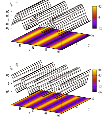
Figure 1: Plots of the OP $\Delta_{ii}$ as a function of position for an s-SC. For (a), $V=2.0$, $h=0.25$; for (b), $V=2.5$, $h=0.4$. Here the chemical potential $\mu=-0.4$.

The OP is calculated self-consistently by solving the BdG equations iteratively, with the OP initially uniform on all sites. The calculation is made on $16\times 16$ supercells each of which is a $32a\times 32a$ lattice and $8\times 32$ supercells each of which is a $64a\times 16a$ lattice, with $a$ the lattice constant. The value of the OP at $H=0$ is determined by the chemical potential $\mu$ and the pairing interaction $V$. The modulation period of the OP is close to $\frac{\pi\hbar v_{f}}{h}$ kakuyanagi , where $v_{f}$ is the Fermi velocity, which is determined by $\mu$. Thus one can adjust the period by changing either $\mu$ or $h$. To change $h$, we have to change $V$ as well, because an FFLO state exists only for $h$ in an interval $[\mu_{0}H_{c1},\mu_{0}H_{c2}]$ FFLO , where $\mu_{0}$ is the magnetic moment of an electron, and the lower and upper critical fields $H_{c1}$ and $H_{c2}$ are both proportional to the superconducting gap at zero $H$. In order to obtain solutions that are commensurate with the lattice, we relax the restriction on $\mu$ and $V$ from the values appropriate to any specific material. Throughout our calculation, we let $t=1$ and $T=0.001$.

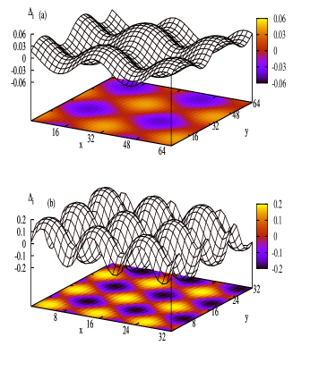
Figure 2: Plots of the OP $\Delta_{i}$ as a functions of position for a d-SC. For (a), $V=1.0$, $h=0.15$ and $\mu=-0.4$; for (b), $V=2.0$, $h=0.4$ and $\mu=-0.4$.

The energetically favored solution in s-SCs always forms 1D stripes, which fits closely to the form $\Delta_{0}\cos(qx)$, with $\Delta_{0}$ the maximum value of the OP which is not necessarily the value of the OP at zero field. We use a $64a\times 16a$ lattice to obtain longer period solutions. Figure 1 shows the OP $\Delta_{ii}$ as a function of position for two choices of $V$ and $h$ at $\mu=-0.4$ for s-SCs. The 1D modulation of the OP with a periodicity $64a/3$ is plotted in Fig. 1(a) with $V=2.0$ and $h=0.25$. Using $V=2.5$, we see in Fig. 1(b) that the periodicity becomes $16a$ at $h=0.4$. We find that the periodicity decreases from $16a$ to $64a/5$ as the Zeeman energy increases from $h=0.4$ to 0.45. For $V=2.0$ and $V=2.5$, the OPs at zero field are $0.34t$ and $0.57t$ respectively. The nodal lines where the OP changes sign are along (010) or the y direction.

The OP of the energetically favored states in d-SCs always forms a square lattice, which fits very closely to the form of $\Delta_{0}[\cos(qx)+\cos(qy)]$, as shown in Fig. 2. As a consequence, the nodal lines of the OP are in (110) and (1$\bar{1}$0) directions. The lattice used for our numerical calculations is $32a\times 32a$. 1D modulation solutions for d-SCs by using a $64a\times 16a$ lattice are also obtained, but they have higher free energy per site than 2D lattice solutions on a $32a\times 32a$ lattice. Fig. 2(a) shows the profile of the OP at $V=1.0$. Here, the OP at zero field is $0.057t$. In order to show the periodic structure of spatial profiles more clearly, for this set of parameters, we have plotted our results on a $64a\times 64a$ lattice by spatial repetition. Fig. 2(b) presents the profile of the OP at $V=2.0$. For this $V$, the OP at zero field is $0.23t$.

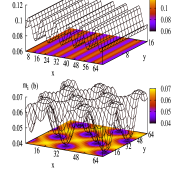
Figure 3: The spatial profile of magnetization $m_{i}$ of the FFLO state. (a) is for an s-SC with $V=2.0$, $h=0.25$ and $\mu$=-0.4. (b) is for a d-SC with $V=1.0$, $h=0.15$ and $\mu=-0.4$.

The magnetization $m_{i}$=$n_{i\uparrow}$-$n_{i\downarrow}$, with $n_{i\uparrow}$ ($n_{i\downarrow}$) as the number of spin-up (-down) electrons at site $i$, has modulations shown in Fig. 3. The parameters of Fig. 3 (a) are the same as those in Fig. 1 (a). The parameters of Fig. 3 (b) are the same as those in Fig. 2 (a). The period of modulation here is one half of that of the OP. The magnetization in an s-SC (a d-SC) forms 1D stripes (2D lattice). The magnitude of the magnetization is highest at the nodal lines of the OP.

The LDOS of spin-up and -down quasi-particles can be calculated from

$$\rho_{i\sigma}(E)=\sum_{n}[|u^{n}_{i\sigma}|^{2}\delta(E_{n}-E)+|v^{n}_{i\bar{\sigma}}|^{2}\delta(E_{n}+E)]$$ (2)

where the delta function $\delta(x)$ has been approximated by $\epsilon/\pi(x^{2}+\epsilon^{2})$. $\epsilon$ is set to 0.01 in our calculation.

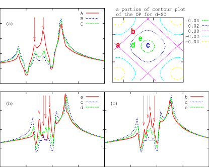
Figure 4: The spin-up LDOS spectrum in the FFLO state. (a): the LDOS at three different locations (A, B, and C, see text,) for an s-SC with $V=2.0$, $h=0.25$ and $\mu=-0.4$. In the upper-right corner, the contour plot of the OP for a d-SC is displayed with five symmetric sites. (b) and (c): Plots similar to (a) for a d-SC with $V=1.0$, $h=0.15$ and $\mu=-0.4$ at sites a, b, c, d and e (see text). The locations of the LDOS peaks are marked by arrows.

In Fig. 4(a), we plot the spin-up LDOS for an s-SC at three sites with reference to Fig. 1(a). Curve A is for a site on the nodal line, curve B is for a site where $|\Delta_{ii}|$ has the maximum absolute value, and curve C is for a midpoint between sites in A and B. In the upper-right corner of Fig. 4, we have the contour plot of the OP for a d-SC with reference to Fig. 2(a). Here a is the saddle point where two nodal lines intersect, b is the mid-site between two neighboring saddle points, c is the site where the OP has the maximum magnitude, and d and e are respectively the mid-points between a-c and b-c. The spin-up LDOS at these symmetric sites are shown in Figs. 4(b) and (c). The spin-down LDOS spectra (not shown) are simply the curves in Fig. 4 shifted to the right by $2h$. Notice that there is a van Hove peak located at $E=0.17$ ($E=0.27$) in Fig. 4(a) [Figs. 4(b) and 4(c)]. The LDOS spectrum is skewed by this van Hove peak. These plots reveal that there are two kinds of ABSs in the d-wave case: One due to the sign change of the OP across the nodal lines, and is similar to the midgap states hu94 . These states would have essentially zero energy if not for the Zeeman shifts to $\mp h$ for spin-up and -down quasiparticles, and broadening into a mini-band due to tunneling between the different nodal lines in a periodic FFLO state. This feature already exist in an s-SC, as shown in Fig. 4(a), and is the signature of a 1D FFLO state. The semiclassical orbit of such a state is a round trip along a straight-line segment across a nodal line, ending with two Andreev reflections involving opposite signs of the OP on the two sides of the nodal line. The same mechanism also gives rise to the inner two peaks in Figs. 4(b) and 4(c) which are for a d-SC. The second kind of ABSs is essentially localized at the saddle points of the OP. Because the FFLO state in d-SC is a 2D lattice, the absolute-OP is very much suppressed in a cross-shaped region at every saddle point, which yields a potential well for a quasiparticle and thus generates two finite-energy ABSs (per spin) at every saddle point. Zeeman shifts also apply to these states, and communication between the saddle points turns these states into two narrow mini-bands. The semiclassical orbits of these states are round trips along straight line segments across the saddle points, ending with two Andreev reflections involving only one sign of the OP. Thus these are not related to the midgap states, and should not have zero energy before Zeeman shift and broadening. The LDOS plot at a saddle point [the curve a in Fig. 4(b)] exhibits two strong peaks corresponding to two ABSs located at $-h\pm\epsilon_{0}$ with $\epsilon_{0}=0.10$, where $-h$ is the Zeeman shift. One can see that curve a is modified by two weak-inner peaks originated in the midgap states. Because of non-locality of these states, 4 low-energy peaks show up at various symmetric points in Figs.4(b) and 4(c). They are located at $E=-0.25$, $-0.17$, $-0.13$ and $-0.05$. (Removing the Zeeman shift there would be at $E=\pm 0.10$ and $\pm 0.02$, representing two $\pm E$ pairs of ABSs of different nature.)

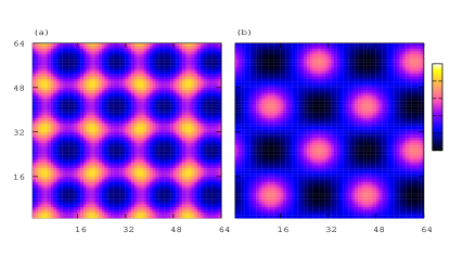
Figure 5: The LDOS maps for spin-up quasiparticles at certain low-energy-peak biases $E$ for d-SC with $V=1.0$, $h=0.15$ and $\mu=-0.4$. For (a), $E=-0.13$. For (b), $E=-0.25$.

For an s-SC, the LDOS map for spin-up quasiparticles at either of the two low-energy peaks, not presented here, forms simple 1D stripes and its intensity is highest at the nodal lines of the OP, as is expected for zero-energy ABS (or midgap states) formed near the nodal lines.

For a d-SC, the structure of the spin-up LDOS maps at the four low-energy-peak biases are richer in physics, and are presented in Figs. 5(a) and 5(b). Fig. 5(a) shows the LDOS map at $E=-0.13$ (with similar result at $E=-0.17$.) The intensity is highest at points on nodal lines halfway between two neighboring saddle points, and is lowest at both the saddle points and the absolute-OP maxima. The high-intensity spots form a $16a\times 16a$ checkerboard pattern with unit vectors along the (100) and (010) directions. Figure 5(b) is at $E=-0.25$ (with similar result if $E=-0.05$). The highest intensity is at saddle points of the OP, and they form a $16\sqrt{2}a\times 16\sqrt{2}a$ checkerboard pattern but the unit vectors are along (110) and $(1{\bar{1}}0)$. Thus the two peaks at $E=-0.17$ and $-0.13$ correspond to zero-energy ABS formed near the nodal lines, similar to the case in the s-SC. On the other hand, the two peaks at $E=-0.25$ and $-0.05$ correspond to finite-energy ABSs formed near the saddle points. Note that if the STM tip is unpolarized, then the measured LDOS should come equally from the spin-up and spin-down contributions. Even under this situation our calculation indicates that the LDOS maps remain qualitatively unchanged as compared to Fig. 5.

In Summary, using a tight-binding model, we have studied, in the low $T$ limit, the FFLO state in a 2D SC with a magnetic field applied in plane. The superconducting OP is self-consistently determined. The spatial profile of the energetically-favored solution is found to form 1D stripes for an s-SC, and a 2D lattice for a d-SC. The spatially-varying magnetization and the quasiparticle LDOS spectrum have been calculated. At all symmetric sites of the FFLO lattice, we find that the low-energy features in the LDOS can be ascribed to two types of ABSs, one is related to zero-energy ABSs (or midgap states) and the other is not. LDOS maps are presented for a d-SC at certain low-energy-peak biases. They are shown to have bias-dependent checkerboard patterns which are different from the spatial profile of the OP. Measuring such maps can clearly reveal the nature of the two different types of ABSs. These characteristics provide clear signatures of the 2D FFLO state in d-SCs. In case the phase of CeCoIn₅ has a competing antiferromagnetic order, we need to use a model suitable for the heavy fermion system to reexamine this problem.

This work is supported by a grant from the Robert A. Welch Foundation under NO. E-1146.

References

- (1) P. Fulde and R. A. Ferrell, Phys. Rev. A 135, 550 (1964); A. I. Larkin and Yu N. Ovchinnikov, Zh. Eksp. Teor. Fiz. 47, 1136 (1964) [Sov. Phys. JETP 20, 762 (1965)].
- (2) K. Maki, Phys. Rev. 148, 362 (1966).
- (3) L. Gruenberg and L. Hunther, Phys. Rev. Lett. 16, 996 (1966).
- (4) A. I. Buzdin and V. V. Tugushev, Sov. Phys. JETP 58, 428 (1983); A. I. Buzdin and S. V. Polonskii, Sov. Phys. JETP 66, 422 (1987).
- (5) H. Burkhardt and D. Rainer, Ann. Phys. 3, 181 (1994).
- (6) M.A. Tanatar et al., Phys. Rev. B 66, 134503 (2002).
- (7) L. Balicas et al., Phys. Rev. Lett. 87, 067002 (2001).
- (8) H. Shimahara, J. Phys. Soc. Jpn. 71, 1644 (2002); H. Shimahara, Physica B 329, 1442 (2003).
- (9) M. Houzet et al., Phys. Rev. Lett. 88. 227001 (2002).
- (10) J. Singleton et al., J. Phys:Condens. Matter 12, L641 (2000).
- (11) K. Izawa et al., Phys. Rev. Lett. 87, 057002 (2001).
- (12) C. Petrovic et al., J. Phys. Cond. Matt. 13, L337 (2001).
- (13) R. Movshovich et al., Phys. Rev. Lett. 86, 5152 (2001).
- (14) A. Bianchi et al., Phys. Rev. Lett. 91, 187004 (2003).
- (15) H. Radovan et al., Nature 425, 51 (2003)
- (16) C. Capan et al., Phys. Rev. B 70, 134513 (2004)
- (17) T. Watanabe et al., Phys. Rev. B 70, 020506(R) (2004).
- (18) C. Martin et al., Phys. Rev. B 71, 020503(R) (2005).
- (19) K. Kakuyanagi et al., Phys. Rev. Lett. 94, 047602 (2005).
- (20) A. B. Vorontsov, J. A. Sauls and M. J. Graf, cond-mat/0506257.
- (21) K. Maki and H. Won, Physica B 322, 315 (2002).
- (22) H. Shimahara, J. Phys. Soc. Japan 67, 736 (1998).
- (23) C.-R. Hu, Phys. Rev. Lett 72, 1526 (1994); Phys. Rev. B 57, 1266 (1998).
- (24) W. Lawrence and S. Doniach, Proceeding of the Twelfth Interational Conference on Low Temperature Physics, E. Kanda (ed.), Academic Press of Japan, Kyoto, 361 (1971).
- (25) J. B. Ketterson and S. N. Song, Superconductivity, Cambridge University Press, Cambridge; New York, 262 (1999).