Effect of microscopic disorder on magnetic properties of metamaterials

Abstract

We analyze the effect of microscopic disorder on the macroscopic properties of composite metamaterials and study how weak statistically independent fluctuations of the parameters of structure elements can modify their collective magnetic response and left-handed properties. We demonstrate that even a weak microscopic disorder may lead to a substantial modification of the metamaterial magnetic properties, and 10% deviation in the parameters of the microscopic resonant elements may lead to a substantial suppression of wave propagation in a wide frequency range. A noticeable suppression occurs also if more than 10% of resonant magnetic elements possess strongly different properties, but in this latter case the defects can create an additional weak resonant line. These results are of the key importance for characterizing and optimizing the novel composite metamaterials with left-handed properties at terahertz and optical frequencies.

I Introduction

Fabricated composite conductive structures for electromagnetic waves or metamaterials acquire a growing attention of researches during the last years due to their unique properties of magnetic permeability and left-handed wave propagation. Being composed of three-dimensional arrays of identical conductive elements, the metamaterials have much in common with conventional optical crystals scaled to support the propagation of microwave or Terahertz radiation. In contrast to crystals, metamaterials allow tailoring their macroscopic properties by adjusting the type and geometry of the structural elements. In particular, it is possible to obtain negative permeability values in magnetically resonant metamaterials at the frequencies up to hundreds of Terahertz NRexp ; tera . This appears to be especially useful for the practical realization of the negative refraction phenomenon Pendry .

The simplest method to create a magnetically resonant metamaterial is to assemble a periodic mesh of the resonant conductive elements (RCEs), where each element is much smaller than the radiation wavelength, and it can be well approximated by a linear LC contour. Introduction of a small slit provides the contour with a certain capacitance while its shape determines the self-inductance. As a result, a resonance of induced currents and corresponding magnetization resonance occurs. Remarkably, the resistive losses in RCEs are low enough to provide the quality factor of the resonance of the order of $10^{3}$ NRexp .

During recent years, a number of ideas have been suggested for achieving better characteristics Tretyakov , tunability PRB ; BG ; Reynet , nonlinear wave coupling PRlow ; ZSK3 ; PRE in composite metamaterials by inserting different types of active and passive electronic complements into the resonant circuits. One of the common features of these seemingly different approaches is to modify the macroscopic properties by identical insertions into the microscopic structure of the metamaterial assuming a technologically ideal fabrication process. It was always assumed that all RCEs are identical, and no analysis of the effect of random deviations or disorder was carried out. However, we should expect that even weak parameter fluctuations in the microscopic parameters may become critical near the magnetic resonance. On the other hand, after a certain operation time, a small amount of RCEs could experience a breakdown operating in a way different from other elements. Thus, the problem of disorder appears naturally in the theory of composite metamaterials.

Recently, the study of defect elements on transmission properties was studied in experiments with one- and two-dimensional metamaterial structures Zhao . The very first study of the effect of disorder in the microscopic structure of metamaterials has been made in Ref. Disorder , where the magnetic susceptibility for a spatially uniform system EPJ has been averaged with respect to random variations of the RCE resonant frequency, and the resulting change of the frequency dispersion of the left-handed composite system has been found analytically. The method used in Ref. Disorder is based on the macroscopic averaging performed prior to the statistical averaging. This is possible only under the assumption that the resonant frequency is a slowly varying random function of coordinate and its correlation length $r_{c}$ satisfies the inequality

$$r_{\text{resp}}\ll r_{c}\ll\lambda,$$ (1)

where $r_{\text{resp}}$ is the characteristic length of the local response (which is usually of the order of a few lattice constants EPJ ), and $\lambda$ is the wavelength of the electromagnetic radiation propagating in the metamaterial. However, the opposite case

$$r_{c}\ll r_{\text{resp}},$$ (2)

appears to be more realistic because even the nearest neighboring RCEs are statistically independent. Then the primary characteristic of the problem is not the average susceptibility itself but the current distribution, and the magnetic properties of the disordered system are determined by a macroscopic average of the current. If the averaging length is large with respect to the correlation length, i.e., if the inequality (2) is fulfilled, then the macroscopic current is a self-averaged quantity LGP , and it should coincide with its ensemble average. In this case, the magnetic properties of the system are described by a statistical mean current.

Below we study systematically the effect of disorder on the averaged characteristics and susceptibility of the metamaterials, and consider two practically important models of the disordered composite metamaterials assuming the capacitances $C_{{\bf n}}$ of different RCEs to be random quantities. In the first model, we assume that the capacitances are completely uncorrelated, i.e. the inequality (2) is automatically satisfied, but the fluctuations are weak. The second model corresponds to small volume density $\tilde{n}$ of inserted defect RCEs acting as impurities with substantially different capacitance $\tilde{C}$. The difference can be very strong here covering two practically important cases of casual RCE breakdown, $\tilde{C}\rightarrow\infty$, and absence of some RCEs, $\tilde{C}\rightarrow 0$. The impurities make the medium microscopically inhomogeneous. The volume in which the local response is formed has to contain a large number of impurities. In accordance with the condition (2), this implies an additional but not very restrictive condition: concentration volume density of impurities should not be extremely small, $\tilde{n}\gg\lambda^{-3}$.

The paper is organized as follows. In Sec. II we develop an appropriate theoretical method based on the response function of the discrete composite medium , which allows describing the properties and response of rather general microscopically inhomogeneous media. Section III is devoted to the study of effects of small deviations in each resonant element. In Sec. IV, we deal with the case of strong but rarefied impurities. Our general conclusions are accompanied by some particular examples calculated numerically for the typical metamaterial parameters. Finally, in Sec. V we discuss the quality and reliability requirements for electronic components to be used as RCE insertions in the composite magnetic metamaterials.

II Response function of magnetic metamaterials

First we consider an ideal composite metamaterial created by a three-dimensional lattice of identical RCEs. The RCEs are placed in the parallel planes normal to the $z$ axis (see Fig. 1), and they form a three-dimensional structure. We denote $N$ the total macroscopic number of the lattice sites with the index ${\bf n}$. For the external fields oscillating with the frequency $\omega$, the relation between the external electromotive forces, $\mathcal{E}_{\bf n}$, applied to RCEs, and the induced currents $I_{\bf n}$ is given by the mutual impedance matrix Landau $\hat{Z}$ with $N^{2}$ elements:

$$\sum_{{\bf m}}Z_{\bf nm}\ I_{\bf m}=\mathcal{E}_{\bf n}.$$ (3)

where $Z_{{\bf n}{\bf m}}=Z({\bf n}-{\bf m})$ for a periodic structure. The diagonal elements of the matrix $\hat{Z}$ coincide with the RCE self-impedance:

$$Z(0)=-i\omega L+\frac{i}{\omega C}+R,$$ (4)

while the non-diagonal ones are determined by the mutual inductance:

$$Z({\bf n}-{\bf m})=-i\omega M({\bf n}-{\bf m})$$ (5)

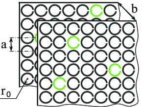
Figure 1: Schematic of two layers of the metamaterial with random insertions of defect resonant elements (shown in green).

We define the discrete Green’s function of the composite metamaterial as the distribution of currents $G(\bf n)$ when only one RCE with the index ${\bf n=0}$ is exposed to the action of the unitary external electro-motive force, i.e. $\mathcal{E}_{\bf n}=\delta_{\bf n,0}$. Then, Eq. (3) yields

$$\sum_{{\bf m}}Z({\bf n-m})G({\bf m-l})=\delta_{\bf n,l}$$ (6)

for arbitrary indices $\bf n$ and $\bf l$. By the other words, discrete Green’s function is the inverse matrix of $\hat{Z}$: $\hat{Z}\hat{G}=\hat{I}.$

The inversion of the difference matrix can be easily performed via the Fourier transform in the reciprocal space. The latter consists of $N$ wave vectors $\bf{k}$ within the first Brillouin zone. We define the Fourier transform $\tilde{f}({\bf k})$ of a discrete function $f({\bf n})$ as

$$\tilde{f}({\bf k})=\frac{1}{N}\sum_{{\bf n}}f({\bf n})e^{-i{\bf k}{\bf n}}$$

so that the inverse transform has the form

$$f({\bf n})=\sum_{{\bf k}}\tilde{f}({\bf k})e^{i{\bf k}{\bf n}}.$$

For the Fourier spectra, using convolution theorem, Eq. (6) reduces to a simple form $Z({\bf k})G({\bf k})=1$, that allows us to write the discrete Green’s function as follows,

$$G({\bf n})=\frac{1}{N}\sum_{{\bf k}}\frac{e^{i{\bf k}{\bf n}}}{\displaystyle{\sum_{{\bf m}}Z({\bf m})e^{-i{\bf k}{\bf m}}}}.$$ (7)

The poles of the Green’s function [i.e. zeros of the denominator in Eq. (7)] determine the spectrum of linear waves that can be excited in the composite metamaterial. In the magnetostatic approximation, only a part of the spectrum can be revealed. Conventional relativistic light-like electromagnetic waves remain beyond the validity of this approach. However, as we demonstrate below, small wave vectors and high group velocities of the light-like waves make their contribution negligible. The excitations which determine the Green’s function on a microscopic scale can be well explored in the magnetostatic approximation. Being first mentioned in Ref. EPJ as Biot-Savart excitons, these linear magnetostatic excitations were named soon magnetoinductive waves Katya1 ; Katya2 . However, these waves can be treated, at least formally, as a classical analogue of linear excitations of spin systems or magnons, and we use the term magnons below in this paper. The spectra of magnons were thoroughly studied in one- and two-dimensional structures. The spectrum of a three-dimensional structure was explored only in the nearest and next-nearest neighbor approximations Katya1 ; Domains , which provide only a qualitative information. As it will be discussed in Sec. III.2 below, in order to obtain a quantitatively reliable results we should take into account hundreds of neighbors.

After changing the summation over the macroscopic number of $\bf k$-vectors by the integration over the first Brillouin zone, $B_{1}$, we obtain

$$G({\bf n})=\frac{1}{(2\pi)^{3}n}\ \int\limits_{B_{1}}\frac{e^{i\bf{kn}}\ d^{3}k}{\displaystyle{\sum_{{\bf m}}Z(\bf m)e^{-i\bf km}}},$$ (8)

where $n$ is the volume density of RCEs. With the help of Eqs. (4), (5) we can rewrite the denominator in the following way

$$G({\bf n})=\frac{i\omega C}{(2\pi)^{3}n}\ \int\limits_{B_{1}}\frac{\Omega^{2}({\bf k})\ e^{i\bf{kn}}\ d^{3}k}{\omega^{2}-\Omega^{2}({\bf k})+i\omega\gamma({\bf k})}.$$ (9)

Here the dispersion $\Omega({\bf k})$ is defined as

$$\Omega^{2}({\bf k})=\frac{\omega_{0}^{2}}{1+L^{-1}\sum\limits_{\bf n}M({\bf n})e^{i\bf kn}},$$ (10)

and the resonance width is

$$\gamma({\bf k})=\frac{\Omega^{2}({\bf k})}{Q\omega_{0}},$$ (11)

where $\omega_{0}=(LC)^{-1/2}$ and $Q=\omega_{0}L/R$ are the RCE resonant frequency and quality factor, respectively.

To isolate the contribution of singular poles, we split the integral in Eq. (9) into the real and imaginary parts,

$$G({\bf n})=\frac{\omega C}{(2\pi)^{3}n}\ \left[A({\bf n})+iB({\bf n})\right],$$ (12)

where the imaginary part allows a straightforward numerical integrating,

$$B({\bf n})=\int\limits_{B_{1}}\frac{\Omega^{2}({\bf k})\left[\omega^{2}-\Omega^{2}({\bf k})\right]\ e^{i{\bf kn}}\ }{\left[\omega^{2}-\Omega^{2}({\bf k})\right]^{2}+\omega^{2}\gamma^{2}({\bf k})}\ d^{3}k,$$ (13)

whereas the real part

$$A({\bf n})=\int\limits_{B_{1}}\frac{\omega\ \Omega^{2}({\bf k})\gamma({\bf k})\ e^{i{\bf kn}}\ }{\left[\omega^{2}-\Omega^{2}({\bf k})\right]^{2}+\omega^{2}\gamma^{2}({\bf k})}\ d^{3}k$$ (14)

has the contribution at the surface $S_{\bf K}$ built by the magnon wave vectors ${\bf K}(\omega)$ obeying the relation $\Omega({\bf K}(\omega))=\omega$. Since the RCE quality factor is high, the singular part dominates in Eq. (14). In the vicinity of the surface $S_{\bf K}$, we write $\Omega({\bf k})\simeq\omega+{\bf k\cdot v(K)}$, where ${\bf v(K)}$ stands for the group velocity. Next, we integrate along the surface normal reducing the volume integration in Eq. (14) to the surface integral over $S_{\bf K}$,

$$A({\bf n})=\pi\omega\int\limits_{S_{\bf K}}\frac{e^{i\bf{Kn}}\ d^{2}K}{v({\bf K})},$$ (15)

which is now more suitable for numerical calculations.

Analyzing Eqs. (13), (15), it is easy to conclude that accounting for the light-like modes would not lead to any noticeable corrections. These modes are located in the center of the Brillouin zone near the point ${\bf k}=0$ and their contribution to the integral $B$ is apparently small. On the other hand, the light group velocity is about two orders of magnitude higher than that of the magnons. Therefore, the light-like part in $A$ is also negligible.

III Weak fluctuations

III.1 Modified magnetic permeability

In order to model the effect of weak disorder in the composite media, we assume that the values of the RCE self-impedances experience random uncorrelated deviations due to the capacitance fluctuations. This may correspond to the results of a real fabrication process when the capacitances of different resonators are not identical, and they can be treated as independent quantities. In this case the correlation radius coincides with the lattice constant, $r_{c}=a$, and the inequality (2) is satisfied. Obviously, strong uncertainty should totally destroy the macroscopic metamaterial response. We assume here that the fluctuations are weak and study their effect on the permeability in the second order of the perturbation theory with respect to capacitance fluctuations, using the methods known from the solid state physics LKTs .

We define the local fluctuations of the RCE impedance as

$$\delta_{{\bf n}}=\frac{1}{\omega}\left(\frac{1}{C_{{\bf n}}}-\frac{1}{C}\right),$$ (16)

where

$$\frac{1}{C}\equiv\bigg{<}\frac{1}{C_{\bf n}}\bigg{>},$$ (17)

where angle brackets stand for statistical averaging. To calculate the magnetic permeability, we follow the procedure described in Ref. EPJ and study the metamaterial exposed to a homogeneous external field ${\bf H}^{(0)}$. Then Eq. (3) takes the form,

$$\sum_{{\bf m}}Z({\bf n}-{\bf m})I_{{\bf m}}+i\delta_{{\bf n}}I_{\bf n}=\mathcal{E},$$ (18)

where $\mathcal{E}=i\mu_{0}\omega SH_{z}^{(0)}$, and $S$ is the RCE area. Iterating Eq. (18), we obtain

$$I_{{\bf n}}=I_{0}-i\sum_{{\bf m}}G({\bf n}-{\bf m})\delta_{{\bf m}}I_{0}-\\ \sum_{{\bf m},{\bf p}}G({\bf n}-{\bf m})G({\bf m}-{\bf p})\delta_{{\bf m}}\delta_{{\bf p}}I_{{\bf p}},$$ (19)

where $I_{0}$ is the current induced in RCEs without parameter fluctuations,

$$I_{0}=\mathcal{E}\sum_{{\bf n}}G({\bf n})=\frac{\mathcal{E}}{Z_{0}},\ \ \ Z_{0}\equiv\sum_{\bf n}Z({\bf n}).$$ (20)

The assumption of weak fluctuations allows us to substitute $I_{0}$ instead of $I_{{\bf p}}$ into the last term of Eq. (19).

The important step in our subsequent analysis is macroscopic averaging of this equation. The size of the (macroscopic) volume of averaging should be small with respect to the wavelength of the external field. On the other hand, this size is much larger than the radius of the capacitance correlations. Therefore, from the statistical point of view, the volume of averaging can be considered infinite. As a result, instead of volume averaging the statistical averaging can be performed LGP . Taking into account that $\langle\delta_{{\bf n}}\rangle=0$, and the capacitances of different RCEs are statistically independent, $\langle\delta_{{\bf m}}\delta_{{\bf p}}\rangle\propto\delta_{{\bf m,p}}$ we obtain that in the second order of the perturbation theory the average current induced in RCEs can be presented as [cf. Eq. (20)]

$$\langle I_{{\bf n}}\rangle=\frac{\mathcal{E}}{Z_{\text{eff}}},$$ (21)

where the effective impedance

$$Z_{\text{eff}}=Z_{0}+\delta^{2}G({\bf 0}),$$ (22)

involves the square of the standard deviation $\delta^{2}=\langle\delta_{\bf n}^{2}\rangle$.

After obtaining the effective impedance, we can perform the rest of the procedure described in Ref. EPJ and finally write the magnetic permeability as follows,

$$\mu_{zz}=\dfrac{iZ_{\text{eff}}-(2/3)\omega\mu_{0}nS^{2}}{iZ_{\text{eff}}+(1/3)\omega\mu_{0}nS^{2}}.$$ (23)

We note that the fluctuations contribute to both imaginary and real parts of $Z_{\text{eff}}$. The imaginary part of the correction is determined by $B({\bf 0})$ and it affects mainly the real part of the permeability. The real part of the correction leads to an increase of $\text{Im}(\mu_{zz})$, i.e., enhances the effective dissipation. Remarkably, this occurs even when RCE losses are absent, and the energy is dissipated without conversion into heating, i.e. this dissipation mechanism is analogous of the Landau damping. The nature of this non-heating dissipation becomes clear if we note that it is determined by the term $A({\bf 0})$, which combines the contributions from all magnetostatic waves excited at the given frequency $\omega$. This suggests that the incident radiation experiences scattering on the microscopic fluctuations. Similar effect arising in electromagnetic media without positional order (see, e.g. Ref. TretBook and references therein) is known as scattering loss or Raleigh scattering. In our case, very small correlation radius suppresses the scattering into light-like modes, but the scattering into magnons is strong.

III.2 Weak disorder in a typical metamaterial

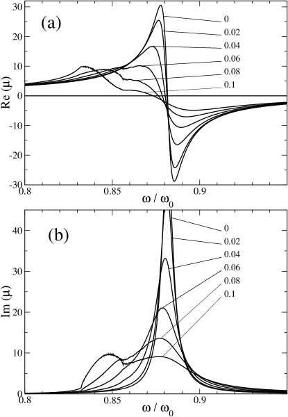
Figure 2: Real (a) and imaginary (b) parts of the magnetic permeability of metamaterial without fluctuations and with weak capacitance fluctuations, $\delta\omega_{0}C$, marked on the plots.

As a particular example of our theory, we calculate the averaged magnetic permittivity numerically for typical metamaterial parameters with a weak disorder. We assume circular RCEs with radius $r_{0}=2\text{mm}$, wire thickness $l=0.1~{}\text{mm}$, which leads to the self-inductance $L=8.36~{}\text{nHn}$ (see Ref. Landau ). To obtain RCEs with the resonant frequency $\omega_{0}=6\pi\cdot 10^{9}\text{rad/s}$ ($\nu_{0}=3\text{GHz}$), we take $C=0.34~{}\text{pF}$. The lattice constants are $a=2.1r_{0}$ in the plane and $b=r_{0}$ in the $z$ direction. The RCE quality factor $Q$ can reach the values of $10^{3}$ NRexp . However, we expect that insertion of diodes or other electronic components can lower this value to $Q=10^{2}$.

First, we calculate the linear spectrum of magnon waves from Eq. (10) and find a strong evidence of long-range interaction effects: the lattice sum converges rather slow. In particular, in order to get an accuracy of a few percent, we have to expand the summation radius to at least ten lattice constants. Further increase of the summation limits would be unjustified since the sum should be calculated over the distances much smaller than the wavelength of radiation. We believe that the problem of exact calculation of magnon spectrum in the three-dimensional case needs a separate detailed consideration. On the other hand, we observe that the maximum uncertainty in the spectrum takes place along specific directions perpendicular to the edges of the Brillouin zone. Therefore, the resulting error in the integrals determining the discrete Green’s function is extremely small.

Evaluating numerically the integrals $A(\bf 0)$ and $B(\bf 0)$ according to Eqs.(13), (15) we obtain the effective impedance and corresponding magnetic permeability. The frequency dispersion of the permeability $\mu_{zz}$ is presented in Fig. 2 for the unperturbed metamaterial and for several values of the standard deviation. Apparently, already a 10% uncertainty changes dramatically the permeability frequency dispersion near the resonance. The effect is most pronounced at the frequencies below the resonance. In a wide range, the imaginary part of $\mu$ becomes comparable with the real part, and the weakly disordered nondissipative medium becomes strongly dissipative. In the range of negative $\mu$ above the resonance, the losses are also considerably higher than in a perfect metamaterial. As a result, the frequency range appropriate for the negative refraction shrinks.

IV Rarefied strong defects

IV.1 Concentration expansion

We consider now the metamaterial with a small amount of randomly distributed defective RCEs which differ strongly from the regular RCEs, and therefore can be treated as impurities. We assume that the dimensionless concentration of impurities $c=\tilde{n}/n$ is low, i.e. $c\ll 1$. As above, we assume that the deviations from the structure parameters appear due to the difference in RCE capacitances, and the capacitance of the impurity, ${\tilde{C}}$, can even become very large corresponding to a casual breakdown. We neglect any correlation between the impurities but assume that two impurities cannot be placed on the same site. The applicability condition, $\tilde{n}\gg\lambda^{-3}$, defines the lower limit for the impurity concentration, $c_{min}\sim 10^{-3}$ for a typical metamaterial. Above this limit, we can calculate statistically averaged current and construct its concentration expansion using standard techniques Lifshits ; LGP .

In the system with impurities, the microscopic current distribution is substantially inhomogeneous. We are interested in the normalized averaged value defined as

$$\langle I\rangle=\frac{1}{N}\sum_{{\bf n}}I_{\bf n},$$ (24)

where the summation is performed over a volume containing a macroscopic number of impurities. The concentration expansion of the averaged current can be written in the following form  Lifshits ; LGP

$$\langle I\rangle=I_{0}+c\sum_{{\bf p}_{1}}\left[I_{1}({\bf p}_{1})-I_{0}\right]+\\ \frac{c^{2}}{2}\sum_{{\bf p}_{1}\neq{\bf p}_{2}}\left[I_{2}({\bf p}_{1},{\bf p}_{2})-I_{1}({\bf p}_{1})-I_{1}({\bf p}_{2})+I_{0}\right]+\ldots.$$ (25)

Here

$$I_{1}({\bf p}_{1})\equiv\frac{1}{N}\sum_{{\bf n}}I_{\bf n}^{(1)}({\bf p}_{1})$$ (26)

is the averaged current if a single impurity is located at the site ${\bf p}_{1}$, while

$$I_{2}({\bf p}_{1},{\bf p}_{2})\equiv\frac{1}{N}\sum_{{\bf n}}I_{\bf n}^{(2)}({\bf p}_{1},{\bf p}_{2})$$

is that for two impurities placed at the sites ${\bf p}_{1},{\bf p}_{2}$. The terms of higher order involve the averaged solutions for more impurities. Clearly, we can write formally the expressions for any term of the expansion Lifshits . However, in this paper we focus on the strongest effects which are linear in the impurity concentration. To calculate the corresponding coefficient, we should find first the corresponding current distribution.

The impedance matrix equation (3) in an impure system exposed to a homogeneous external field takes the form

$$\sum_{{\bf m}}Z({\bf n}-{\bf m})I_{{\bf m}}+i\Delta\sum_{{\bf p}}\delta_{{\bf n,p}}\ I_{{\bf p}}=\mathcal{E},$$ (27)

where the summation in the second term in the l.h.s. is performed over the impurity sites ${\bf p}$ only, and

$$\Delta=\frac{1}{\omega}\left(\frac{1}{\tilde{C}}-\frac{1}{C}\right).$$ (28)

Inverting the matrix $\hat{Z}$, we rewrite Eq. (27) as follows,

$$I_{{\bf n}}=I_{0}-i\Delta\sum_{{\bf p}}G({\bf n}-{\bf p})I_{{\bf p}}.$$ (29)

If a single impurity is located at the site ${\bf p}_{1}$, Eq. (29) taken at ${\bf n}={\bf p}_{1}$ yields

$$I_{{\bf p}_{1}}=\frac{I_{0}}{1+i\Delta G({\bf 0})}$$ (30)

and the current distribution in this case is

$$I_{{\bf n}}^{(1)}({\bf p}_{1})=I_{0}\left[1-\frac{i\Delta G({\bf n}-{\bf p}_{1})}{1+i\Delta G({\bf 0})}\right].$$ (31)

Averaging this expression according to Eq.(26) and substituting the result into Eq. (25) leads to the same results (21) and (23) for the averaged current and the magnetic permeability correspondingly, where the effective impedance is

$$Z_{\text{eff}}=Z_{0}+c\ \frac{i\Delta}{1+i\Delta G({\bf 0})}.$$ (32)

IV.2 Effective magnetic permeability

To illustrate our results with a specific example, we take typical parameters of metamaterials used above in Sec. III.2. First, we study the effect of impurities with an infinite capacitance, $\tilde{C}\rightarrow\infty$, which corresponds, for instance, to a casual breakdown of varactor diode insertions. Next, we deal with other impurities which either do not contribute to the magnetization or are just absent; this latter case is modelled by setting $\tilde{C}\rightarrow 0$. Although these cases are two opposite extreme limits, the resulting averaged permeabilities look similar and differ only by few percents. This result is not surprising, because in both cases the currents induced in the defect RCEs are either small or vanish.

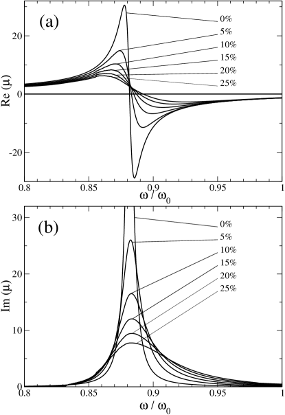
Figure 3: (a) Real and (b) imaginary parts of the magnetic permeability of metamaterials without and with impurities (impurity concentration is shown near the curves).

In Fig. 3 we present the real and imaginary parts of the magnetic permeability for several concentrations of missing RCEs. As follows from those results, the resonance is attenuated much more than one could expect from the fact that a small part of RCEs do not contribute to the resonance. The reasons for that enhancement are scattering losses which decrease the effective quality factor by an order of magnitude or more. We see also that the metamaterial is more sensitive to such perturbations in the frequency range of negative $\mu$. The composite medium can tolerate 5% or less malfunctioning RCEs, but for 10% and more a substantial damping of the resonance occurs, and the imaginary part of the permeability becomes comparable with the real one.

The impurities with a finite resonant frequency, $\tilde{\omega}_{0}\neq 0$, which strongly differs from the main frequency $\omega_{0}$, cause observable effects even if their concentration is extremely low. As seen in Fig. 4, only 1% of such impurities can build up their own weak resonance, with the position of the resonance shifted from the impurity eigenfrequency.

In the linear approximation used here, the effect of mutual interaction of impurities is neglected. Therefore, we are not accounting for the magnons arising at frequencies close to the impurity resonance. We expect that the corresponding scattering losses will broaden the resonance. However, the detailed analysis of this and related phenomena is beyond the scope of this paper.

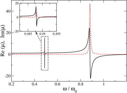
Figure 4: (color online) Real (solid) and imaginary (dashed) parts of the permeability of metamaterial with 1% of randomly distributed defects with the eigenfrequency $\tilde{\omega}_{0}=0.5\omega_{0}$. The inset shows a blow up of the impurity resonance.

V Concluding remarks

We have demonstrated that even a weak microscopic disorder in the conducting elements of composite metamaterials can lead to a substantial modification of their resonant magnetic response. According to our results, already 10% disorder in the parameters causes substantial scattering of the incident radiation into magnetization waves. This modifies strongly the macroscopic permeability of the metamaterial leading to the increase of losses. We believe the study of disorder and effective losses is of a critical importance for engineering novel metamaterials with various electronic elements inserted into their microscopic resonators. The inserted elements should possess no more than a few percent deviation of their capacitance and/or inductance to ensure that the metamaterial properties are not distorted dramatically. Another restriction concerns the insertion stability. The data obtained demonstrate that the metamaterial tolerates no more than 10% disorder in the parameters of the resonant conductive elements. Casual breakdown of a greater part of the insertions causes strong damping of the wave propagation in metamaterials.

Our results that even a small amount of defects can build up a noticeable additional magnetic resonance look useful for suggesting a simple methods for the sensitive quality control of metamaterials. If an RCE contains not a single capacitive element but a combination of insertions with an ordinal slit, a casual insertion breakdown would switch the RCE to another resonant frequency. The corresponding narrow gap (or peak) in the metamaterial transmission can be used as a sensitive indicator of the concentration of damaged RCEs.

Finally, we point out that the effects of microscopic disorder would be crucially important in the nanostructured metamaterials even with simple RCEs without electronic components. Clearly, the fabrication of resonant elements on such scales is less accurate, so that random fluctuations of the RCE shapes can lead to deviations of the self-inductance and capacitance. Disorder in position of RCEs determines the deviations of mutual inductance. We expect that the results obtained here can be important for qualitative estimations of nanostructured left-handed media. However, the problem requires a separate and more systematic analysis.

References

- (1) R.A. Shelby, D.R. Smith, and S. Schultz, Science 292, 77 (2001).
- (2) S. Linden, C. Enkrich, M. Wegener, J.F. Zhou, T. Koschny, and C.M. Soukoulis, Science 306, 1351 (2004).
- (3) J.B. Pendry, Phys. Rev. Lett. 85, 3966 (2000).
- (4) S.A. Tretyakov, Microwave and Opt. Techn. Lett. 31, 163 (2001).
- (5) M. Gorkunov and M. Lapine, Phys. Rev. B 70, 235109 (2004).
- (6) S. O’Brien, D. McPeake, S.A. Ramakrishna, and J.B. Pendry, Phys. Rev. B 69, 241101(R) (2004).
- (7) O. Reynet and O. Acher, Appl. Phys. Lett. 84, 1198 (2004).
- (8) M. Lapine, M. Gorkunov, and K.H. Ringhofer, Phys. Rev. E 67, 065601(R) (2003).
- (9) A.A. Zharov, I.V. Shadrivov, and Yu.S. Kivshar, Phys. Rev. Lett. 91, 037401 (2003).
- (10) M. Lapine and M. Gorkunov, Phys. Rev. E 70, 066601 (2004).
- (11) X.P. Zhao, Q. Zhao, L. Kang, J. Song, and Q.H. Fu, Phys. Lett. A (2005).
- (12) A.A. Zharov, I.V. Shadrivov, and Yu.S. Kivshar, J. Appl. Phys. 97, 113906 (2005).
- (13) M. Gorkunov, M. Lapine, E. Shamonina, and K.H. Ringhofer, Eur. Phys. J. B 28, 263 (2002).
- (14) I.M. Lifshits, S.A. Gredeskul, and L.A. Pastur, Introduction to the Theory of Disodered Systems (New York, Wiley, 1989).
- (15) L.D. Landau and E.M. Lifschitz, Electrodynamics of Continuous Media (Pergamon Press, Oxford, 1984).
- (16) E. Shamonina, V.A. Kalinin, K.H. Ringhofer, and L. Solymar, J. Appl. Opt. 92, 6252 (2002).
- (17) M.C.K. Wiltshire, E. Shamonina, I.R. Young, and L. Solymar, Electron. Lett. 39, 215 (2003).
- (18) I.V. Shadrivov, A.A. Zharov, N.A. Zharova, and Yu.S. Kivshar, cond-mat/0501653 (2005).
- (19) I.M. Lifshitz and L.N. Rosentsveig, Zh. Eksp. Teor. Fiz. 16, 967 (1946).
- (20) S. Tretyakov, Analytical Modelling in Applied Electromagnetics (Artech House, Boston, 2003).
- (21) I.M. Lifshits, Nuovo Cim. Suppl. 3, 716 (1956).