Surfaces of Constant Temperature in Time

Abstract

The inverse relationship between energy and time is as familiar as Planck’s constant. From the point of view of a system with many states, perhaps a better representation of the system is a vector of characteristic times (one per state) for example, in the case of a canonically distributed system. In the vector case the inverse relationship persists, this time as a relation between the $L_{2}$ norms. That relationship is derived herein. An unexpected benefit of the vectorized time viewpoint is the determination of surfaces of constant temperature in terms of the time coordinates. The results apply to all empirically accessible systems, that is situations where details of the dynamics are recorded at the microscopic level of detail. This includes all manner of simulation data of statistical mechanical systems as well as experimental data from actual systems (e.g. the internet, financial market data) where statistical physical methods have been applied.

Surfaces of Constant Temperature in Time David Ford
Naval Postgraduate School
Monterey, California

I Introduction

Perhaps the most obvious relation between energy and time is given by the expression for the energy of a single photon $E=\hbar\nu$. In higher dimensions a similar energy-time relation

$$\|H\|_{2}=\frac{const.}{\|t\|_{2}}$$

holds for the $L_{2}$ norms of state energies and characteristic times associated with a canonically distributed system. This relationship is made precise herein. A by-product of the result is the possibility of the determination of surfaces of constant temperature given sufficient details about the trajectory of the system through its path space.

As an initial value problem, system kinetics are determined once an initial state and energy function are specified. In the classical setting, representative cell occupation numbers may be assigned any compact region of position, $\mathbf{q}$, momentum, $\mathbf{p}$, space Uhlenbeck and Ford (1963). An important model of a quantum system is provided by lattices of the Ising type Glauber (1963), Mazenko et al. (1978). Here the state of the system is typically specified by the configuration of spins.

Importantly, two systems that share exactly the same state space may assign energy levels to those states differently. In the classical context one may, for example, hold the momenta fixed and vary the energy by preparing a second system of slower moving but more massive particles. In the lattice example one might compare systems with the same number of sites but different coupling constants, etc.

Consider a single large system comprised of an ensemble of smaller subsystems which all share a common, finite state space. Let the state energy assignments vary from one subsystem to the next. Equivalently, one could consider a single, fixed member of the ensemble whose Hamiltonian, $H_{subsystem}$, is somehow varied (perhaps by varying external fields, potentials and the like Schrodinger (1989)). Two observers, A and B, monitoring two different members of the ensemble, $\mathcal{E}_{A}$ and $\mathcal{E}_{B}$, would accumulate the same lists of states visited but different lists of state occupation times. The totality of these characteristic time scales, when interpreted as a list of coordinates (one list per member of the ensemble), sketch out a surface of constant temperature in the shared coordinate space.

II Restriction on the Variations of $H_{subsystem}$

From the point of view of simple arithmetic, any variation of $H_{subsystem}$ is permissible but recall there are constraints inherent in the construction of a canonical ensemble. Once an energy reference for the subsystem has been declared, the addition of a single constant energy uniformly to all subsystems states will not be allowed.

Translations of $H_{subsystem}$ are temperature changes in the bath. The trajectory of the total system takes place in a thin energy shell. If the fluctuations of the subsystem are shifted uniformly then the fluctuations in the bath are also shifted uniformly (in the opposite direction). This constitutes a change in temperature of the system. This seemingly banal observation is not without its implications. The particulars of the situation are not unfamiliar.

A similar concept from Newtonian mechanics is the idea of describing the motion of a system of point masses from the frame of reference of the mass center. Let $\{H_{1},H_{2},\ldots,H_{N}\}$ be the energies of an $N-$state system. A different Hamiltonian might assign energies to those same states differently, say $\{\tilde{H}_{1},\tilde{H}_{2},\ldots,\tilde{H}_{N}\}$. To describe the transition from the energy assignment $\mathbf{H}$ to the assignment $\mathbf{\tilde{H}}$ one might first rearrange the values about the original ‘mass center’

$$\frac{H_{1}+H_{2}+\ldots+H_{N}}{N}$$ (1)

and then uniformly shift the entire assembly to the new ‘mass center’

$$\frac{\tilde{H}_{1}+\tilde{H}_{2}+\ldots+\tilde{H}_{N}}{N}.$$ (2)

In the present context, the uniform translations of the subsystem state energies are temperature changes in the bath. As a result, the following convention is adopted. For a given set of state energies $\{H_{1},H_{2},\ldots,H_{N}\}$, only those changes to the state energy assignments that leave the ‘mass center’ unchanged will be considered in the sequel.

The fixed energy value of the “mass center” serves as a reference energy in what follows. For simplicity this reference is taken to be zero. That is

$$H_{1}+H_{2}+\ldots+H_{N}=0.$$ (3)

Uniform translation will be treated as a temperature fluctuation in what follows. An obvious consequence is that only $N-1$ subsystem state energies and the bath temperature $\theta$ are required to describe the statistics of a canonically distributed system.

III Two One-Dimensional Subspaces

In the event that a trajectory of the subsystem is observed long enough so that each of the $N$ states is visited many times, it is supposed that the vector of occupancy times spent in state, $\{\Delta t_{1},\Delta t_{2},\ldots,\Delta t_{N}\}$, is connected to any vector of N-1 independent state energies and the common bath temperature, $\{H_{1},H_{2},\ldots,H_{N-1},\theta\}$, by relations of the form

$$\frac{\Delta t_{k}}{\Delta t_{j}}=\frac{e^{-\frac{H_{k}}{\theta}}}{e^{-\frac{H_{j}}{\theta}}}$$ (4)

for any $k,j\in\{1,2,\ldots,N\}$. The value of the omitted state energy, $H_{N}$, is determined by equation (3).

The number of discrete visits to at least one of these states will be a minimum. Select one of these minimally visited states and label it the rare state. The observed trajectory may be decomposed into cycles beginning and ending on visits to the rare state and the statistics of a typical cycle may be computed. For each $k\in\{1,2,\ldots,N\}$, let $\Delta t_{k}$ represent the amount of continuous time spent in the $k^{th}$ state during a typical cycle. In the Markoff setting the $L_{1}$ norm

$$\sum_{k=1}^{N}\Delta t_{k}=\textrm{characteristic system time},$$ (5)

may serve as the Carlson depth. These agreements do not affect the validity of equation (4).

At finite temperature, it may be the case that the system is uniformly distributed. That is, the observed subsystem trajectory is representative of the limiting case where the interaction Hamiltonian has been turned off and the subsystem dynamics take place on a surface of constant energy.

In the left hand panel of figure 1, the $\theta-$axis coincides with the set of all state energies and bath temperatures corresponding to uniformly distributed systems. In the time domain, the ray containing the vector $\mathbf{1}$ (see the right hand panel) depicts the set of state occupancy times that give rise to uniformly distributed systems.

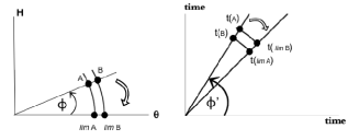
Figure 1: Schematic of the approach to the uniform distribution for dilatation pairs in both the energy and time domains.

For real constants $c_{\Delta t}$ and $c_{E}$ scale transformations of the type

$$\Delta\mathbf{t}\longrightarrow c_{\Delta t}\;\;\Delta\mathbf{t}$$

$$\{\mathbf{H},\theta\}\longrightarrow c_{E}\;\{\mathbf{H},\theta\}$$

dilatate points along rays in their respective spaces and leave equation (4) invariant.

The left hand panel of figure 1 shows a pair of energy, temperature coordinates: A and B, related by a dilatation scale factor $c_{E}$, rotated successively toward the coordinates $lim\,A$ and $lim\,B$ which lie on the line of uniform distribution (the $\theta$ axis) in the energy, temperature domain. Throughout the limit process (parameterized by the angle $\phi$) the scale factor $c_{E}$ is held constant. Consistent with the relations in equation (4), the points $t(A)$ and $t(B)$ (putative time domain images of the given energy, temperature domain points A and B) as well as the image of their approach to the uniform distribution in time ($\phi^{\prime}=cos^{-1}(\frac{1}{\sqrt{N}})$, where N is the dimensionality of the system), are shown in the right hand panel of the same figure.

As the angle of rotation $\phi^{\prime}$ (the putative image of $\phi$ in the time domain) is varied, there is the possibility of a consequent variation of the time domain dilatation scale factor $c_{\Delta t}$ that maps $t(A)$ into $t(B)$. That is, $c_{\Delta t}$ is an unknown function of $\phi^{\prime}$. However in the limit of zero interaction between the subsystem and the bath the unknown time domain scaling, $c_{\Delta t}$, consistent with the given energy, temperature scaling, $c_{E}$, is rather easily obtained.

At any step in the limit process as $\phi^{\prime}$ approaches $cos^{-1}(\frac{1}{\sqrt{N}})$ equation (4) implies that

$$\frac{\Delta t(B)_{k}}{\Delta t(B)_{j}}=\frac{\Delta t(A)_{k}}{\Delta t(A)_{j}}$$ (6)

for any $k,j\in\{1,2,\ldots,N\}$.

Assuming, as the subsystem transitions from weakly interacting to conservative, that there are no discontinuities in the dynamics, then equations (4) and (6) hold along the center line $\phi^{\prime}=cos^{-1}(\frac{1}{\sqrt{N}})$ as well.

In the conservative case with constant energy $H_{ref}$, the set identity

$$\{(\mathbf{q},\mathbf{p}):\mathbf{H}(\mathbf{q},\mathbf{p})-H_{ref}=0\}\equiv\{(\mathbf{q},\mathbf{p}):c_{E}\;(\mathbf{H}(\mathbf{q},\mathbf{p})-H_{ref})=0\}$$ (7)

together with scaling behavior of the position and momentum velocities given by Hamilton’s equations

$$\begin{split}\mathbf{\dot{q}(A)}\rightarrow&c_{E}\,\mathbf{\dot{q}(A)}\\ \mathbf{\dot{p}(A)}\rightarrow&c_{E}\,\mathbf{\dot{p}(A)}\end{split}$$ (8)

illustrate that the phase space trajectory associated with the energy, temperature domain point $limB$ is simply the trajectory at the point $limA$ with a time parameterization “sped up” by the scale factor $c_{E}$. See figure 2. This identifies the the scale factor associated with the points $t(limB)$ and $t(limA)$ as

$$\lim_{\phi^{\prime}\rightarrow cos^{-1}(\frac{1}{\sqrt{N}})}c_{\Delta t}(\phi^{\prime})=\frac{1}{c_{E}}.$$ (9)

Figure 2: The trajectory is everywhere tangent to both $\mathbf{H}$ and $\mathbf{c_{E}H}$ vector fields.

IV Matched Invariants Principle and the Derivation of the Temperature Formula

A single experiment is performed and two observers are present. The output of the single experiment is two data points (one per observer): a single point in in the $\Delta t$ space and a single point in the $(H;\theta)$ space.

In the event that another experiment is performed and the observers repeat the activity of the previous paragraph, the data points generated are either both the same as the ones they produced as a result of the first experiment or else both are different. If a series of experiments are under observation, after many iterations the sequence of data points generated traces out a curve. There will be one curve in each space.

$\it{The\;principle\;follows}$: in terms of probabilites, the two observers will produce consistent results in the case when the data points (in their respective spaces) have changed from the first experiment to the second but the probabilites have not. That is, if one observer experiences a dilatation so does the other.

Of course, if the observers are able to agree if dilatation has occurred they are also able to agree that it has not. In terms of probability gradients, in either space the dilatation direction is the direction in which all the probabilities are invariant. In the setting of a system with N possible states, the N-1 dimensional space perp to the dilatation is spanned by any set of N-1 probability gradients. We turn next to an application of the MIP.

Consider two points $\theta_{1}$ and $\theta_{2}$ along a ray colocated with the temperature axis in the $(H,\theta)$ space. Suppose that the ray undergoes a rigid rotation (no dilatation) and that in this way the two points are mapped to two new points $A$ and $B$ along a ray which makes an angle $\phi$ with the temperature axis. See the left hand panel of figure 3.

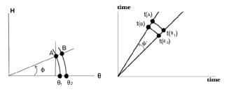
Figure 3: The temperature ratio is invariant with respect to rotation in either space

It’s pretty obvious that the temperature ratio is preserved throughout the motion. For whatever the angle $\phi$

$$\frac{\theta_{1}}{\theta_{2}}=\frac{\theta_{1}\;cos(\phi)}{\theta_{2}\;cos(\phi)}=\frac{\theta(A)}{\theta(B)}.$$ (10)

Let $t(\theta_{1})$ and $t(\theta_{2})$ be the images in the time domain of the points $\theta_{1}$ and $\theta_{2}$ in $(H,\theta)$ space. According to the matched invariants principle, since the rotation in $(H,\theta)$ space was rigid so the corresponding motion as mapped to the time domain is also a rigid rotation (no dilatations). See figure 3.

More precisely, to the generic point $A$ in $(H,\theta)$ space with coordinates $(H_{1},H_{2},\ldots,H_{N},\theta)$ associate a magnitude, denoted $\|\mathbf{H}\|$, and a unit vector $\hat{\mathbf{e}}_{\mathbf{H}}$. Recall that the $H$’s live on the hyperplane $H_{1}+H_{2}+\cdots+H_{N}=0.$ It will be convenient to express the unit vector in the form

$$\hat{\mathbf{e}}_{\mathbf{H}}=\frac{\{\frac{H_{1}}{\theta},\frac{H_{2}}{\theta},\ldots,\frac{H_{N}}{\theta},1\}}{\sqrt{(\frac{H_{1}}{\theta})^{2}+(\frac{H_{2}}{\theta})^{2}+\cdots+(\frac{H_{N}}{\theta})^{2}+1}}.$$ (11)

The angle between that unit vector and the temperature axis is determined by

$$cos(\phi)=\hat{\mathbf{e}}_{\theta}\cdot\hat{\mathbf{e}}_{\mathbf{H}}$$ (12)

where $\hat{\mathbf{e}}_{\theta}=\{0,0,\ldots,0,1\}$.

The temperature at the point $A$, is the projection of its magnitude, $\|\mathbf{H}_{A}\|$, onto the temperature axis

$$\theta(A)=\|\mathbf{H}_{A}\|\,cos(\phi).$$ (13)

Another interpretation of the magnitude $\|\mathbf{H}_{A}\|$ is as the temperature at the point $\theta_{1}$, the image of $A$ under a rigid rotation of the ray containing it, on the temperature axis. See figure 3. With this interpretation

$$\theta(A)=\theta_{1}\,cos(\phi).$$ (14)

An easy consequence of equation (3) is

$$\frac{H_{k}}{\theta}=\log[\frac{(\prod_{j=1}^{N}p_{j})^{\frac{1}{N}}}{p_{k}}].$$ (15)

In terms of the occupation times

$$\frac{H_{k}}{\theta}=\log[\frac{(\prod_{j=1}^{N}\Delta t_{j})^{\frac{1}{N}}}{\Delta t_{k}}].$$ (16)

An easy implication of equation (9) is that

$$\sqrt{\sum_{j=1}^{N}\Delta t_{j}^{2}}=\frac{\textrm{const.}}{\theta_{1}}.$$ (17)

for an arbitrary but fixed constant carrying dimensions of $\textrm{time}\cdot\textrm{energy}$.

Together equations (14), (16), and (17) uniquely specify the surfaces of constant temperature in time

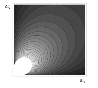
Figure 4: The constant temperature surfaces for a two dimensional system.

$$\theta(\Delta\mathbf{t})=\frac{\textrm{const.}}{\|t\|_{2}\,\sqrt{(\log[\frac{\prod}{\Delta t_{1}}])^{2}+(\log[\frac{\prod}{\Delta t_{2}}])^{2}+\cdots+(\log[\frac{\prod}{\Delta t_{N}}])^{2}+1}}$$ (18)

where,

$$\prod=(\Delta t_{1}\cdot\Delta t_{2}\ldots\Delta t_{N})^{\frac{1}{N}}.$$ (19)

The temperature formula (18) may be recast into the more familiar form

$$\|H\|_{2}=\frac{const.}{\|t\|_{2}}$$ (20)

With the temperature determined, equation (16) gives the state energies of a canonically distributed subsystem. From these, a wealth of useful macroscopic properties of the dynamics may be computed Ford (2004). Surfaces of constant temperature for a two state system are shown in figure 4.

References

- Uhlenbeck and Ford (1963) G. E. Uhlenbeck and G. W. Ford, Lectures in Statistical Mechanics. Proceedings of the Summer Seminar, Boulder, Colorado, Vol.1 (American Mathematical Society, 1963).
- Glauber (1963) R. Glauber, Time Dependent Statistics of the Ising Model (J. Math. Physics 4, 2, 1963).
- Mazenko et al. (1978) G. Mazenko, M. Nolan, and O. Valls, Application of Real-Space Renormalization Group to Dynamic Critical Phenomena (Phys Rev Lett 41, 7, 1978).
- Schrodinger (1989) E. Schrodinger, Statistical Thermodynamics (Dover, 1989).
- Landau and Lifshitz (1980) L. D. Landau and E. M. Lifshitz, Statistical Physics (Pergamon, 1980).
- Ford (2004) D. Ford (2004), eprint cond-mat/0402325.