The effect of collective spin-1 excitations on electronic spectra in high-$T_{c}$ superconductors

Abstract

We review recent experimental and theoretical results on the interaction between single-particle excitations and collective spin excitations in the superconducting state of high-$T_{c}$ cuprates. We concentrate on the traces, that sharp features in the magnetic-excitation spectrum (measured by inelastic neutron scattering) imprint in the spectra of single-particle excitations (measured e.g. by angle-resolved photoemission spectroscopy, tunneling spectroscopy, and indirectly also by optical spectroscopy). The ideal object to obtain a quantitative picture for these interaction effects is a spin-1 excitation around 40 meV, termed ’resonance mode’. Although the total weight of this spin-1 excitation is small, the confinement of its weight to a rather narrow momentum region around the antiferromagnetic wavevector makes it possible to observe strong self-energy effects in parts of the electronic Brillouin zone. Notably the sharpness of the magnetic excitation in energy has allowed to trace these self-energy effects in the single-particle spectrum rather precisely. Namely, the doping- and temperature dependence together with the characteristic energy- and momentum behavior of the resonance mode has been used as a tool to examine the corresponding self-energy effects in the dispersion and in the spectral lineshape of the single-particle spectra, and to separate them from similar effects due to electron-phonon interaction. This leads to the unique possibility to single out the self-energy effects due to the spin-fermion interaction and to directly determine the strength of this interaction in high-$T_{c}$ cuprate superconductors. The knowledge of this interaction is important for the interpretation of other experimental results as well as for the quest for the still unknown pairing mechanism in these interesting superconducting materials.

Contents

1. Introduction 1
2. Experimental evidence of a sharp collective spin excitation and its coupling to fermions 2
   2.1. Inelastic Neutron Scattering 2.1
        2.1.1. Magnetic coupling 2.1.1
        2.1.2. The magnetic resonance feature 2.1.2
        2.1.3. Bilayer effects 2.1.3
        2.1.4. Temperature dependence 2.1.4
        2.1.5. Doping dependence 2.1.5
        2.1.6. Dependence on disorder 2.1.6
        2.1.7. Isotope effect 2.1.7
        2.1.8. Dependence on magnetic field 2.1.8
        2.1.9. The incommensurate part of the spectrum 2.1.9
        2.1.10. The spin gap 2.1.10
        2.1.11. The spin fluctuation continuum 2.1.11
        2.1.12. Normal state spin susceptibility 2.1.12
   2.2. Angle resolved photoemission 2.2
        2.2.1. Fermi surface 2.2.1
        2.2.2. Normal-state dispersion and the flat-band region 2.2.2
        2.2.3. MDC and EDC 2.2.3
        2.2.4. Bilayer splitting 2.2.4
        2.2.5. Superconducting coherence 2.2.5
        2.2.6. EDC-derived dispersion anomalies 2.2.6
        2.2.7. The $S$-shaped MDC-dispersion anomaly 2.2.7
        2.2.8. The nodal kink 2.2.8
        2.2.9. Fermi velocity 2.2.9
        2.2.10. Spectral lineshape 2.2.10
        2.2.11. The antinodal quasiparticle peak 2.2.11
        2.2.12. The spectral dip feature 2.2.12
        2.2.13. Real part of self energy: renormalization of dispersion 2.2.13
        2.2.14. Imaginary part of self energy: quasiparticle lifetime 2.2.14
        2.2.15. Isotope effect 2.2.15
        2.2.16. Relation to pseudogap phase 2.2.16
   2.3. C-axis tunneling spectroscopy 2.3
   2.4. Optical spectroscopy 2.4
3. The collective mode as spin-1 exciton 3
   3.1. Theoretical models 3.1
   3.2. Characteristic energies 3.2
   3.3. The resonance mode 3.3
        3.3.1. Development of spin exciton 3.3.1
        3.3.2. Doping dependence 3.3.2
        3.3.3. Dependence on disorder 3.3.3
        3.3.4. Dependence on magnetic field 3.3.4
        3.3.5. Even and odd mode in bilayer cuprates 3.3.5
   3.4. The incommensurate response 3.4
   3.5. Effective low-energy theories 3.5
   3.6 Magnetic coherence in La_2-xSr_xCuO₄ 3.6
4. Coupling of quasiparticles to the magnetic resonance mode 4
   4.1. The coupling constant and the weight of the spin resonance 4.1
   4.2. Theoretical model 4.2
        4.2.1. Tight binding fit to normal state dispersion 4.2.1
        4.2.2. Model spectrum and basic equations 4.2.2
   4.3. Contribution from the spin fluctuation mode 4.3
        4.3.1. Characteristic electronic scattering processes 4.3.1
        4.3.2. Electronic self energy 4.3.2
        4.3.3. Renormalization function and quasiparticle scattering rate 4.3.3
        4.3.4. Spectral functions at the $M$ point 4.3.4
   4.4. Contribution of the spin fluctuation continuum 4.4
   4.5. Renormalization of EDC and MDC dispersions 4.5
   4.8. Bilayer splitting 4.6
   4.6. Tunneling spectra 4.7
   4.8. Doping dependence 4.8
5. Discussion of phonon effects 5
6. Open problems 6
7. Conclusions 7
Acknowledgements 8
References References

1 Introduction

Cuprate high-$T_{c}$ superconductivity, discovered in 1986 [1], arises when a sufficient amount of charge carriers (holes or electrons) is doped into an antiferromagnetic, Mott-insulating parent compound [2, 3]. It is one of the fields which continues to inspire both theoretical and experimental research. The development of new methods and the improvement of existing ones as a result of the research in cuprate superconductivity have influenced many other fields in condensed-matter physics. However, there is no generally accepted agreement about the pairing mechanism in these materials, and not even the normal state has been described in a satisfactory way up to date.

Due to dramatic improvements in the resolution in angle-resolved photoemission (ARPES) experiments during the last years, the properties of single-particle electronic excitations throughout the Brillouin zone have been thoroughly studied. An agreement has emerged that at least in the superconducting state electronic quasiparticle excitations are well defined [4, 5] and are the entities participating in superconducting pairing [6]. However, there are numerous anomalies, caused by self-energy effects, which complicate the dispersions and spectral lineshapes observed in ARPES experiments.

The recent developments in testing fermionic single-particle excitations in high-$T_{c}$ cuprate superconductors were to a large extend driven by a suggestion that several dispersion anomalies observed in angle-resolved-photoemission experiments can be explained in a unified picture invoking a strong coupling to a resonant magnetic mode at antiferromagnetic wavevector $(\pi,\pi)$, which is observed in inelastic-neutron-scattering experiments [7]. In this scenario, the finite momentum width of the resonance mode plays a crucial role, leading to scattering of quasiparticles that is maximal for points in the Brillouin zone separated by a $(\pi,\pi)$ wavevector, but to a less extend also present for scattering between points separated by a wavevector deviating from $(\pi,\pi)$. This crucial generalization of a model by Kampf and Schrieffer [8] allowed to explain the variety of observed effects in one single model.

The self-energy effects in the single-particle dispersions, which are being studied experimentally in great detail, open a unique possibility to determine the crucial parameters for a successful theoretical description of the high-$T_{c}$ phenomenon, namely the strength of the coupling between the electronic single-particle excitations and the collective excitations due to lattice modes (phonons) as well as electronic modes present in the spin-, charge- or pairing channel. The knowledge of these interaction strengths is pivotal for a correct theoretical description of both the normal and superconducting state of cuprate superconductors.

Numerous experimental techniques have been used to analyze collective excitations of various types. For example, inelastic neutron scattering (INS) is a direct probe of both the phonon spectrum and of the spectrum of electronic collective excitations. In particular, it is possible by spin-polarized INS techniques to separate electronic excitations of magnetic origin from non-magnetic excitations. The experimental results obtained in this way are the second crucial ingredient for the determination of the relevant coupling constants for electronic excitations in cuprates. Namely, in order to assign the correct collective excitations to the various self-energy effects observed by ARPES techniques, it is necessary to compare the temperature- and doping dependence of the self-energy effects with that of the corresponding collective modes observed by INS techniques. Only if both the energy range and the magnitude of the observed dispersion anomalies match the energy and intensity of the corresponding collective excitations, is it possible to extract the necessary information for the interaction constants.

Motivated by earlier work [8, 9, 10, 11, 12, 13, 14, 15, 16], a thorough study along these lines has emerged during the last years, which has found a clear correlation between the spin-fluctuation spectrum measured in INS experiments and the self-energy effects measured in ARPES experiments [17, 18, 19, 20, 21, 22, 23, 7, 24, 25, 26, 27, 28, 29, 30, 31]. This theoretical development stimulated great experimental interest. In particular, it led to doping- and temperature dependent studies of the self-energy effects related to the magnetic resonance excitation by ARPES experiments [32, 33, 34, 35, 36, 37, 38, 39, 40, 41, 42, 43], tunneling spectroscopy [44], and optical spectroscopy [45].

It turned out that it was also necessary to analyze the momentum dependence of the self-energy effects and to relate them to the momentum-width of the collective spin excitation [7, 25] in order to be able to distinguish it clearly from other collective modes like for example phonons. In high-$T_{c}$ cuprates phonons are generally accepted to couple to electrons in a moderate way, and on theoretical grounds phononic features should be observable in the single-particle spectra as well. Corresponding effects have been found and have been examined experimentally by INS [46, 47, 48] and ARPES [49, 50, 51, 52, 53, 54] as well as theoretically (see [55, 56, 57], and references therein). We concentrate in this review on the interaction of electronic single-particle excitations with collective spin excitations in cuprates. It has been shown e.g. by inelastic neutron scattering and by spatially resolved NMR techniques, that spin fluctuations play an important role not only above $T_{c}$ but also in the superconducting vortex state [58, 59, 60, 61]. The results of INS and ARPES experiments as well as other experimental techniques, as tunneling spectroscopy and optical spectroscopy, and the correlation between the data obtained from these different techniques, allowed for the first time a rather direct and precise determination of the coupling strength between conduction electrons and spin collective excitations in cuprate systems.

The dominant interaction for single-particle electronic excitations (quasiparticles) in three-dimensional metals and superconductors is the electron-phonon interaction. In contrast, for lower-dimensional systems the interaction between quasiparticles and collective electronic excitations becomes relevant. This is a direct result of the Pauli exclusion principle, which leads to stronger kinematic phase-space restrictions in higher dimensions. In quasi-twodimensional materials single particle excitations are in general modified (but not completely destroyed) by interactions with collective modes [62] (this is unlike to quasi-onedimensional materials where the interactions between single particle excitations and collective excitations are dominating the physics). It is therefore not surprising that in high-temperature cuprate superconductors, which are quasi-twodimensional materials, such collective excitations have a strong impact on quasiparticles. Experimentally it was observed, that at least in the superconducting state quasiparticle-like excitations are well defined, and to a large extend can be successfully described by a $d$-wave modification of the Bardeen-Cooper-Schrieffer theory of superconductivity [63]. The normal state of high-temperature superconductors poses more problems in this respect. For this reason the study of the homogeneous superconducting state might be easier than that of the normal state, and might give some support for the more difficult tasks of understanding the pseudogap phase and inhomogeneous superconducting phases. Thus, we concentrate in this review on the superconducting state and refer the reader for the interesting questions of the normal-state and pseudogap-state behavior to other reviews [64, 65, 66]. In Fig. 1 the typical phase diagram for the cuprate superconductors as a function of hole-doping is shown.

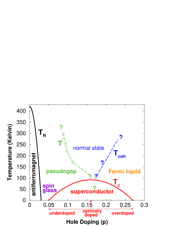
Figure 1: Typical phase diagram for high-$T_{c}$ cuprates over the number of doped holes per Cu ion, $p$. Superconductivity arises when the antiferromagnetic parent compound ($p=0$) is doped with a certain amount of charge carriers (here holes). Optimal doping corresponds to the doping value with highest $T_{c}$. The circles are recent data from Ref. [67] of an additional transition observed in neutron scattering experiments. Question marks denote regions of the phase diagram that are theoretically not well understood. (After Refs. [66, 67])

Superconductivity can also be achieved by electron doping. In this review, however, we restrict ourselves to the hole-doped materials, as the vast majority of INS and ARPES experiments were performed for those. So far in the experimental investigations of electron-doped cuprates the characteristic self-energy effects as well as the resonance mode in the spin excitation spectrum that are the main topic of this review have not been found.

We start in Section 2 with a review of the available experimental data, concentrating on the most recent data referring to self-energy effects observed by ARPES experiments and spin-collective modes observed by INS experiments. Then, in Section 3 we review theoretical developments concerning the interpretation of the collective spin-excitation as spin-1 excitonic mode below the spin-fluctuation continuum. In Section 4 we review the methods used to extract the interaction effects between the single-particle excitations and the collective spin-1 excitonic excitations from available experimental data. Using the results of INS experiments and normal state parameters obtained from ARPES experiments, the various self-energy effects observed in the superconducting state by ARPES and tunneling experiments are then compared with the theoretical results and are shown to give a consistent picture. Section 5 is devoted to the discussion on self-energy effects due to electron-phonon interaction. Finally, in Section 6 we discuss open problems and in Section 7 we summarize the important implications of this field of high-$T_{c}$ research for an understanding of superconductivity in these systems.

2 Experimental evidence of a sharp collective spin excitation and its coupling to fermions

2.1 Inelastic Neutron Scattering

Neutron scattering experiments have been important in the study of collective excitations in high-temperature superconductors. Inelastic neutron scattering experiments probe both collective excitations of the lattice (phonons) and collective excitations of the electronic system. In typical metals such electronic collective excitations are small perturbations to the liquid of quasiparticles above the Fermi sea ground state. The reason for this is, that the dynamics of single-particle excitations for such liquids can be described by a quantum transport equation for many body excitations which have signatures of single particles. In three dimensional systems, the only collective excitations which affect the collision terms of the transport equation in leading order in a controlled approximation are phonons. Cuprates are quasi-twodimensional, and it was shown that in two-dimensional systems quasiparticle collision terms are governed by electronic collective excitations even far from instabilities [62, 68]. But still, in these cases, the equilibrium properties of such quasi-twodimensional systems are expected to be unaffected by collective electronic modes in leading order in $T/E_{F}$, as long as singular corrections are not important in higher orders. For the importance of such singular corrections in two dimensions see Ref. [69] and references therein. In cuprates equilibrium properties show unusual behavior at least in the normal state [64]. Thus, it is possible that collective electronic modes play an important role even for equilibrium properties. Examples for such electronic modes are spin fluctuations (as a precursor for spin wave modes), charge fluctuations (precursor for density waves), combinations of both (‘stripes’, [70, 71, 72, 73, 74, 75, 76, 77, 78]), pair fluctuations, and combinations of all of those modes with lattice deformations (’polarons’).

There has been an enormous amount of work in revealing the properties of magnetic excitations in these materials. The magnetic part of the inelastic neutron scattering (INS) signal is usually much smaller than the signal from e.g. phonons, and special techniques had to be applied in order to extract it. Fortunately the magnetic response is strongly enhanced near the antiferromagnetic wavevector in cuprate superconductors, which allowed for an experimental analysis of the magnetic excitation spectrum in cuprates. The main focus of this study has been a strong peak at the antiferromagnetic wavevector, which is sharp in energy and has for optimally doped materials an excitation energy near 40 meV. We will concentrate in the following on the magnetic excitation spectrum observed in INS in the superconducting state of high-$T_{c}$ materials, with particular weight on the above-mentioned sharp resonant mode.

2.1.1 Magnetic coupling

In cuprate superconductors the superconducting structural units are either one single copper oxide layer or several closely spaced copper oxide layers. These units are separated by much larger distances than the layers within such units. Correspondingly, there is a hierarchy of magnetic superexchange couplings.

The in-plane magnetic superexchange coupling $J_{\parallel}$ is of the order of 120-150 meV. In the antiferromagnetic insulating state it can be obtained experimentally by fitting the spin wave velocity to quantum Monte-Carlo calculations. In La₂CuO₄ this procedure gave $J_{\parallel}=133$ meV [79].

The superexchange between different superconducting units is more than four orders of magnitude smaller than the primary coupling within one copper oxygen plane, $J_{\parallel}$. It is of the order of 0.02 meV [80, 81]. Inelastic neutron scattering experiments show that the neutron scattering signal in the metallic state of cuprates can be described by an incoherent superposition of the signals from different superconducting units. Thus, these units can be considered as magnetically decoupled. This is expected on theoretical grounds from the fact that the magnetic in-plane correlation lengths in cuprates are only a few lattice spacings.

The coupling $J_{\perp}$ between different planes within a superconducting unit, however, is only one order of magnitude less than $J_{\parallel}$, $J_{\perp}\sim 10$ meV [82]. Even in the metallic regime a strong magnetic coupling $J_{\perp}$ remains [81, 83, 84, 85]. This coupling is e.g. reflected in a pronounced $Q_{z}$-dependence of the inelastic neutron scattering signal for bilayer cuprates [85]. The corresponding signal is proportional to the imaginary part of the susceptibility

$$\chi({\bf Q},Q_{z},\omega)=\sum_{ij}e^{iQ_{z}(z_{i}-z_{j})}\chi^{ij}({\bf Q},\omega)$$ (1)

where

$$\chi^{ij}({\bf Q},\omega)=\langle T_{\tau}\hat{S}_{z}^{i}({\bf Q},\tau)\hat{S}_{z}^{j}(-{\bf Q},0)\rangle$$ (2)

with the spin-density operator $\hat{S}_{z}^{i}({\bf Q})=\sum_{{\bf k},\alpha\beta}c^{\dagger}_{i,{\bf k}+{\bf Q},\alpha}\;\hat{\sigma}^{z}_{\alpha\beta}\;c_{i,{\bf k},\beta}$ (here, ${\bf Q}$ and ${\bf k}$ are in-plane vectors). The fact that a pronounced $Q_{z}$-dependence is observed both in the normal and superconducting state indicates that there is no significant change in coherence between the planes within a bilayer due to onset of superconductivity [85].

The magnetic part of the spectrum measured in inelastic neutron scattering experiments describes the spectrum of spin fluctuations. In the superconducting state of cuprates it typically consists of three parts. The first is a continuum, which is gapped at low energies. The main feature for cuprates with $T_{c}$ around 90 K is a resonance feature peaked at the antiferromagnetic wave vector, and is present at energies below the continuum. Below the resonance energy, an incommensurate response develops [86, 87, 88], which however never extends to zero energy, but instead the spectrum is limited at low energies by the so called spin gap $E_{sg}$ [89]. As also above the resonance an incommensurate response is observed, the incommensurate response in superconducting cuprates shows a typical hour-glass shape [90, 91, 92, 93].

2.1.2 The magnetic resonance feature

The magnetic resonance mode was first observed in inelastic neutron scattering experiments for bilayer cuprates in the superconducting state, with energy near 40 meV in optimally doped compounds [94, 95, 96, 97, 98, 99]. This resonance is sharp (resolution limited, where the instrumental resolution is typically less than 10 meV) in energy and magnetic in origin [95]. It is centered in momentum around the antiferromagnetic wavevector ${\bf Q}=(\pi,\pi)$. In contrast to its sharpness in energy, in momentum the resonance has a finite width of typically $0.25\AA^{-1}$ (full width half maximum, FWHM).

The total momentum width of the spectrum is minimal at the resonance energy [100, 98], where it is (in contrast to the off-resonant momentum width) only weakly doping dependent, with a full momentum width of about $0.22\AA^{-1}$ [100, 101, 89]. This corresponds to a correlation length $\xi_{sfl}$ of about two lattice spacings. Note, however, that the spectrum above and below the resonance consists of incommensurate peaks which strongly overlap, and thus the total momentum width overestimates the momentum width of the incommensurate spin excitations.

A similar resonance feature is also observed in underdoped YBa₂Cu₃O_6+x, but at reduced energy [102, 103, 104, 106, 105]. Also in Bi₂Sr₂CaCu₂O_8+δ the resonance was found both in the optimally doped [99, 107] and overdoped [107] regime. For a comparison with tunneling and ARPES data, which were predominantly performed on Bi₂Sr₂CaCu₂O_8+δ, it is important to notice that the characteristic features are very similar to those for YBa₂Cu₃O_6+x.

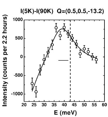
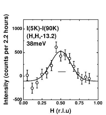
Figure 2: Magnetic resonance in the odd channel for overdoped Bi₂Sr₂CaCu₂O_8+δ ($T_{c}$=83 K). The difference spectra of the INS intensity measured at 5 K and 90 K at the antiferromagnetic wavevector as a function of energy shows a resonance peak at 38 meV (left picture). The constant energy scans at resonance energy, shown in the right picture, shows that the resonance is concentrated near the antiferromagnetic wavevector, however with a finite momentum width given in relative lattice units (i.e. units of inverse lattice constant). (From Ref. [107], Copyright ©2001 APS)

In Fig. 2 the INS data for overdoped Bi₂Sr₂CaCu₂O_8+δ are reproduced [107]. The dashed line in the left panel of Fig. 2 indicates the resonance energy for an optimally doped Bi₂Sr₂CaCu₂O_8+δ sample. Also the instrumental resolution is shown. The momentum width, shown in the right picture of Fig. 2 is somewhat broader than that for YBa₂Cu₃O_6+x.

Importantly, the resonance has not only been observed in bilayered cuprates, but also in the single layered cuprate Tl₂Ba₂CuO_6+δ [108]. Thus, it is not a specific feature of closely spaced layers within a unit cell, but an intrinsic property of the whole superconductor.

In the normal state these systems show a much weaker response, which is centered around ${\bf Q}=(\pi,\pi)$ and is broader in momentum than in the superconducting state. In the pseudogap state, some intermediate picture is observed, with a gradually sharpening response at the antiferromagnetic wavevector, which can be regarded as a precursor of the magnetic resonance mode below $T_{c}$ [109, 110, 89].

The resonant feature has not been observed in the single-layered system La_2-xSr_xCuO₄. In contrast, in this compound the magnetic excitations are strong both in the normal and superconducting state and located at incommensurate planar wave vectors ${\bf Q}_{\delta}=(\pi(1\pm\delta)),\pi)$ and $(\pi,\pi(1\pm\delta))$ [111, 112, 90, 113]. These incommensurate peaks are enhanced and sharpen in momentum at low energies ($E<5k_{B}T_{c}$) when entering the superconducting state [112]. However, it was recently shown [114] that a dispersion similar to that in YBa₂Cu₃O_6+x does also exist in optimally doped La_2-xSr_xCuO₄. In this case, however the maximal intensity is at the low-energy incommensurate part of the dispersion spectrum. The recent experiments [114, 115] support the idea that the resonance peak in the 90 K cuprates and the incommensurate response in the La_2-xSr_xCuO₄ possibly have a common origin.

The characteristic parameters for the resonance feature are summarized in Tab. 2.1.2 for the different studied compounds. In this table, the intensity of the mode $W({\bf Q})$ at the antiferromagnetic wavevector is defined by $W=\int{\rm d}\omega{\rm Im}\chi({\bf Q},\omega)$, and $\langle W({\bf Q})\rangle$ denotes the momentum average of $W({\bf q})$ over the entire Brillouin zone.

Characteristic parameters for the resonance feature in different cuprate superconductors as determined by inelastic neutron scattering experiments at low temperatures ($T\ll T_{c}$). Here, D is the doping (o=overdoped, u=underdoped, op=optimally doped), $S$ denotes the symmetry with respect to the exchange of the layers within the unit cell (e=even, o=odd), $\Omega_{res}$ is the resonance frequency, $\Delta Q$ its FWHM momentum width, $W({\bf Q})$ its weight at the antiferromagnetic wave vector, and $\langle W({\bf Q})\rangle$ denotes the momentum averaged resonance intensity. Ref. compound D $T_{c}$ S $\Omega_{res}$ $\Delta Q$ $W({\bf Q})$ $\langle W({\bf Q})\rangle$ [K] [meV] [$\AA^{-1}$] [$\mu_{B}^{2}/{\rm f.u.}$] [$\mu_{B}^{2}/{\rm f.u.}$] [109] YBa₂Cu₃O₇ op 93 o 40 0.25 1.6 0.043 [118] Y_0.85Ca_0.15Ba₂Cu₃O₇ o 75 o 34 0.45 e 35 0.18 [116] Y_0.9Ca_0.1Ba₂Cu₃O₇ o 85.5 o 36 0.36 1.2^∗ 0.042 [118]^∗ e 43 0.45 0.6^∗ 0.036 [92] YBa₂Cu₃O_6.85 u 89 o 41 0.25 1.8^∗ 0.07^† [118]^∗ e 53 0.41 0.55^∗ [109]^† [118] YBa₂Cu₃O_6.6 u 63 o 37 2.0 e 55 0.2 [109] YBa₂Cu₃O_6.7 u 67 o 33 0.25 2.1 0.056 [109] YBa₂Cu₃O_6.5 u 52 o 25 0.25 2.6 0.069 [117] YBa₂(Cu_0.97Ni_0.03)₃O₇ 80 o 35 0.49 1.6 0.2 [119] YBa₂(Cu_0.995Zn_0.005)₃O₇ 87 o 40 0.25 2.2 0.056 [117] YBa₂(Cu_0.99Zn_0.01)₃O₇ 78 o 38 0.44 [99] Bi₂Sr₂CaCu₂O_8+δ op 91 o 43 0.52 1.9 0.23 [107] Bi₂Sr₂CaCu₂O_8+δ o 83 o 38 [108] Tl₂Ba₂CuO_6+δ op 92.5 - 47 0.23 0.7 0.02

2.1.3 Bilayer effects

In doubly layered materials, under the assumption of coherent coupling between the planes within a bilayer, the dispersion is classified by the notion of bonding bands (BB) and antibonding bands (AB). In contrast, if the coupling is predominantly incoherent, a classification according to the layer index is more appropriate.

Because of the symmetry under exchange of the planes within a bilayer, the susceptibility $\chi_{ij}$ (where $i,j=1,2$ are layer indices) has only two independent components, $\chi_{\parallel}\equiv\chi_{11}=\chi_{22}$ and $\chi_{\perp}\equiv\chi_{12}=\chi_{21}$ [120]. Using those, the neutron scattering cross section for bilayer cuprates is given by

$$\frac{d^{2}\sigma}{d\Omega dE}\sim F^{2}({\bf Q})\left[\chi^{\prime\prime}_{\parallel}({\bf Q},\omega)+\cos(Q_{z}d)\chi^{\prime\prime}_{\perp}({\bf Q},\omega)\right],$$ (3)

where $\chi^{\prime\prime}_{\parallel,\perp}({\bf Q},\omega)$ is the imaginary part of the dynamical magnetic susceptibility within and between the layers, respectively, $d\approx 3.3\AA$ is the distance between the CuO₂ planes within a bilayer, and $F({\bf Q})$ is the magnetic form factor of the Cu²⁺ ion [109].

It is common to introduce components for excitations even and odd under interchange of planes within a bilayer, $\hat{S}_{z}^{e}=(\hat{S}_{z}^{1}+\hat{S}_{z}^{2})/2$ and $\hat{S}_{z}^{o}=(\hat{S}_{z}^{1}-\hat{S}_{z}^{2})/2$. The corresponding even and odd susceptibilities are,

$$\chi_{e} \equiv \langle T_{\tau}\hat{S}_{z}^{e}({\bf Q},\tau)\hat{S}_{z}^{e}(-{\bf Q},0)\rangle=\chi_{\parallel}({\bf Q},\omega)+\chi_{\perp}({\bf Q},\omega)$$ (4)

$$\chi_{o}({\bf Q},\omega) \equiv \langle T_{\tau}\hat{S}_{z}^{o}({\bf Q},\tau)\hat{S}_{z}^{o}(-{\bf Q},0)\rangle=\chi_{\parallel}({\bf Q},\omega)-\chi_{\perp}({\bf Q},\omega).$$ (5)

The neutron scattering cross section for bilayer cuprates is given in terms of even and odd susceptibilities by,

$$\frac{d^{2}\sigma}{d\Omega dE}\sim F^{2}({\bf Q})\Big{[}\sin^{2}(\frac{Q_{z}d}{2})\chi^{\prime\prime}_{o}({\bf Q},\omega)+\cos^{2}(\frac{Q_{z}d}{2})\chi^{\prime\prime}_{e}({\bf Q},\omega)\Big{]},$$ (6)

where $\chi^{\prime\prime}_{o/e}({\bf Q},\omega)$ is the imaginary part of the dynamical magnetic susceptibility in the odd and even channels, respectively [109].

In the case of coherent coupling of the planes within a bilayer the more appropriate classification is in terms of susceptibilities within the basis of bonding ($b$) and antibonding ($a$) bands. In this case, the odd susceptibility component describes scattering between opposite type of bands, and the even susceptibility describes scattering between same type of bands, according to [85]

$$\chi_{e}({\bf Q},\omega) = \frac{1}{2}\left[\chi_{aa}({\bf Q},\omega)+\chi_{bb}({\bf Q},\omega)\right]$$ (7)

$$\chi_{o}({\bf Q},\omega) = \frac{1}{2}\left[\chi_{ab}({\bf Q},\omega)+\chi_{ba}({\bf Q},\omega)\right].$$ (8)

The spin resonance was for a long time only observed in the odd channel [81], where it lies below a gapped continuum, the latter having a signal typically a factor of 30 less than the maximum at ${\bf Q}$ at the mode energy [83]. The continuum is gapped in both the even and odd scattering channels (the even channel is gapped by $\approx 60$ meV even in the normal state) [82].

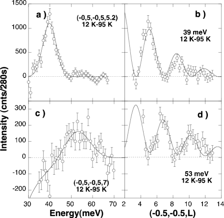
Figure 3: Differences of the INS intensity measured at 12 K and 95 K for an underdoped YBa₂Cu₃O_6.85 sample ($T_{c}=89$ K, [92]). a) and b) are for the odd channel, c) and d) for the even channel. The INS intensity as function of energy shows resonance peaks at 39 meV in the odd channel and at 53 meV in the even channel. The constant energy scans at resonance energy, shown in b) and d), reveal the typical sin-square modulation for the odd-channel mode and the cos-square modulation for the even-channel mode (full lines). (From Ref. [92], Copyright ©2004 APS).

Recently the resolution of neutron scattering experiments has increased considerably to allow for the observation of the resonance mode also in the channel even with respect to the layer-interchange within a bilayer. The corresponding mode has been observed in both overdoped and underdoped YBa₂Cu₃O_7-δ [116, 92, 118]. As shown in Fig. 3 b) and d) for underdoped YBa₂Cu₃O_6.85, the dependence of the magnetic INS signal as function of $Q_{z}$ shows the characteristic sin-squared and cos-squared modulations for the odd and even channels, respectively [92]. The corresponding resonance energies, as obtained from Fig. 3 a) and c), are 39 meV in the odd channel, and 53 meV in the even channel. The intensity in the even channel is much smaller than in the odd channel, which is the reason why it was for such a long time overlooked.

The peak energy in overdoped Y_0.9Ca_0.1Ba₂Cu₃O₇ for the odd channel is at 36 meV, lower than the mode energy in optimally doped YBa₂Cu₃O_7-δ. The corresponding peak width in momentum space around ${\bf Q}=(\pi,\pi)$ is $\Delta Q=0.36\pm 0.05\AA^{-1}$. The even channel resonance mode is at 43 meV, and has a $Q$-width of $\Delta Q=0.45\pm 0.05\AA^{-1}$. The intensity data of the two modes are shown in Table 2.1.2.

2.1.4 Temperature dependence

A sharp resonance mode is not observed above $T_{c}$ [96, 110]. However, a broadened version is present in the pseudogap state [89], which can be regarded as a pre-cursor for the resonance. On approaching $T_{c}$ from below the resonance energy does not change [98, 96, 102], however its intensity is vanishing toward $T_{c}$ for optimally doped compounds, following an order parameter like behavior [94, 95, 98, 102, 110]. The temperature dependence of the even and odd resonance mode intensity is, when properly rescaled, identical [116, 92]. This is shown in Fig. 4 for moderately underdoped YBa₂Cu₃O_6.85 and overdoped Y_0.9Ca_0.1Ba₂Cu₃O₇. The peak amplitude of both the even and odd mode vanish at $T_{c}$.

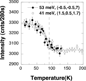
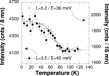
Figure 4: Temperature dependence of the neutron scattering intensity at the antiferromagnetic wavevector for the resonance mode in the even channel (full circles) and in the odd channel (open circles). The even mode intensity has been rescaled to that of the odd mode. The measurements were performed by INS in underdoped YBa₂Cu₃O_6.85 (left picture, $T_{c}$=89 K, [92]) and overdoped Y_0.9Ca_0.1Ba₂Cu₃O₇ (right picture, $T_{c}$=85.5 K, [116]) YBa₂Cu₃O_7-δ. (From Refs. [116], Copyright ©2003 APS, and [92], Copyright ©2004 APS).

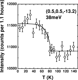
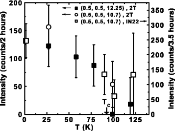
Figure 5: Temperature dependence of the neutron scattering intensity at the antiferromagnetic wavevector for the odd-channel resonance mode in overdoped Bi₂Sr₂CaCu₂O_8+δ (left picture, $T_{c}$=83 K, [99, 107]) and for the single layered compound Tl₂Ba₂CuO_6+δ near optimal doping (right picture, $T_{c}$=90 K, [108]). (From Ref. [107], Copyright ©2001 APS, and Ref. [108], Reprinted with permission from Science, Ref. [108]. Copyright ©2002 AAAS).

When going to stronger underdoped samples, the INS intensity at resonance energy and antiferromagnetic wavevector is present also above $T_{c}$ up to a temperature which characterizes pseudogap phenomena in cuprates [106]. This correlates with other thermodynamic quantities like the specific heat as function of temperature for different degrees of doping [106]. It was argued, that a similar correspondence exists also as a function of applied magnetic field [121, 122].

The characteristic temperature dependence of the mode intensity was observed also in overdoped Bi₂Sr₂CaCu₂O_8+δ [99, 107] and in the single layered compound Tl₂Ba₂CuO_6+δ near optimal doping, as shown in Fig. 5.

2.1.5 Doping dependence

The width of the resonance in the odd channel is smaller than the instrumental resolution (of typically less than 10 meV) for optimally and moderately underdoped materials. Strongly underdoped materials show a small broadening of the order of 10 meV [83, 109]. The mode frequency decreases with underdoping and has its maximal value of about 40 meV at optimal doping [102, 103, 104, 106]. In both underdoped and overdoped regimes, the resonance energy, $\Omega_{res}$, is proportional to $T_{c}$ with $\Omega_{res}\approx(5\ldots 5.5)k_{B}T_{c}$ [83, 109, 106, 99, 107].

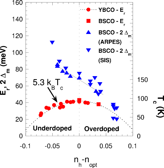
Figure 6: Doping dependence of magnetic-resonance energy, $\Omega_{res}$ ($\equiv E_{r}$), as measured by INS in YBa₂Cu₃O_7-δ [94, 95, 96, 98, 109, 89], and Bi₂Sr₂CaCu₂O_8+δ [99, 107]. For comparison, twice the maximal superconducting gap, $\Delta_{m}$, for Bi₂Sr₂CaCu₂O_8+δ, as determined from ARPES [123] and from SIS tunneling [44], is shown. (From Ref. [124], Copyright ©2004 WILEY-VCH).

In Fig. 6 we reproduce the data from Ref. [124]. As can be seen the resonance-mode energy tracks very precisely the curve for 5.3 $T_{c}$. Also shown are the values for twice the maximal superconducting gap as determined from ARPES [123] and from SIS break junctions tunneling data [44]. The resonance feature stays always below this continuum edge, indicating an excitonic origin. The doping dependence in Fig. 6 should be compared with the right panel in Fig. 41. The similarity is striking.

The total spectral weight related to the resonance peak remains approximately constant as a function of doping, and amounts to 0.06$\mu_{B}^{2}$ per formula unit at low temperatures [106, 109]. This represents about 2% of the spectral weight contained in the spin-wave spectra of the undoped materials. With underdoping the intensity of the resonance at ${\bf q}=(\pi,\pi)$ increases from about 1.6 $\mu_{B}^{2}$ for YBa₂Cu₃O₇ to about 2.6 $\mu_{B}^{2}$ per unit volume for YBa₂Cu₃O_6.5 [83, 109]. With overdoping, the intensity at the antiferromagnetic wavevector decreases, however there are no data available for strongly overdoped samples.

2.1.6 Dependence on disorder

In cuprates the superconducting transition temperature can be varied also without changing the carrier concentration by introducing disorder through impurity substitution in the CuO₂-layers. Due to the unconventional energy gap such impurities have a strong effect on equilibrium properties of the superconducting state, in contrast to conventional $s$-wave superconductors. Two types of impurities were used in substitution for Cu²⁺ ions in inelastic neutron scattering experiments. First, non-magnetic Zn²⁺ ions ($3d^{10},S=0$ configuration) [119, 117], and second, magnetic Ni²⁺ ions ($3d^{8},S=1$ configuration) [125, 117]. In general, the influence on the superconducting transition temperature of non-magnetic impurities is stronger than the influence of magnetic impurities in cuprates. The $T_{c}$ reduction is 3 times stronger for Zn²⁺ ions than for Ni²⁺ ions [126, 127]. It was found that for YBa₂(Cu_1-yNi_y)₃O₇ with $y=3\%$, $T_{c}=80$K, the resonance shifted to lower energy, preserving the ratio $\Omega_{res}/k_{B}T_{c}$, whereas for YBa₂(Cu_1-yZn_y)₃O₇ the shift of the resonance energy with impurity doping is much smaller [125, 117]. The intrinsic energy width of the resonance peak is very sensitive to both types of impurities, being $\Delta E=11$meV for YBa₂(Cu_0.997Ni_0.003)₃O₇ and $\Delta E=9$meV for YBa₂(Cu_0.999Zn_0.001)₃O₇ [117]. However, there are differences in the temperature dependence of the magnetic response function for the two types of impurities. Whereas Ni impurities do not measurably enhance the normal state response, a broad peak with characteristic energy somewhat lower than the resonance energy of pure YBa₂Cu₃O₇ appears in the normal state for systems containing Zn impurities [117].

2.1.7 Isotope effect

Very recently also the influence of an change of the oxygen isotope was studied in YBa₂Cu₃O_6.89 [128]. It was shown, that there is no shift in the resonance frequency when exchanging the oxygen isotope ¹⁶O by ¹⁸O. This shows the absence of interaction between the spin-1 excitation and phonons in high-$T_{c}$ cuprates near optimal doping. However, the amplitudes of the peaks are slightly different, and also the energy widths differ slightly; the energy integrated magnetic spectral weight, however, stays unaffected. This modifications could possibly be related to a certain amount of introduced disorder due to isotope exchange.

2.1.8 Dependence on magnetic field

It was found that a c-axis magnetic field suppresses the intensity of the magnetic resonance [122], as predicted from an analysis of specific heat data [121]. Since the same effect was not observed for in-plane fields [129], this indicates that the resonance is sensitive to the presence of Abrikosov vortices, and thus intimately connected to the nature of the superconducting ground state. This has obvious implications for microscopic theories of the resonance.

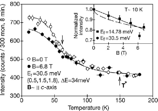
Figure 7: Effect of the magnetic field on the temperature dependence of the magnetic resonance intensity and field dependence of the resonance intensity in underdoped YBa₂Cu₃O_6.6 ($T_{c}=$ 62.7 K, odd resonance energy $\Omega_{res}=$ 34 meV) at the antiferromagnetic wavevector at $T\sim 10$K [122]. The magnetic field points in $c$-axis direction. Open circles are for zero field, full circles for $B=$6.8 T ($E_{f}$ denotes the final neutron energy). The inset shows the magnetic field dependence of the normalized resonance intensity at 10 K, the solid line corresponds to $I/I_{0}=1-(B/\mbox{36 T})$. The characteristic field of 36 T is not far from the upper critical field $B_{c2}=$45 T for this sample. (Reprinted with permission from Mcmillan Publishers Ltd: Nature, Ref. [122], Copyright ©2000 NPG).

As shown in the inset of Fig. 7, the experimental suppression goes like $1-H/H^{*}$, which is highly suggestive of a vortex core effect, as originally noted by Dai et al. [122]. It is interesting to remark that the sample studied experimentally had an anomalously long magnetic correlation length. Other samples studied by neutron scattering have a significantly smaller correlation length [89]. This fact probably lead to a larger effect of the magnetic field on the magnetic resonance than in other samples, allowing its experimental observation. The resulting temperature dependence for the resonance intensity with and without applied magnetic field is reproduced in Fig. 7. As the sample is strongly underdoped, there is a considerable magnetic intensity at the resonance energy left even above $T_{c}$, as mentioned in Subsection 2.1.4. The suppression of the mode intensity with magnetic field in $c$-direction is clearly visible below $T_{c}$.

2.1.9 The incommensurate part of the spectrum

There has been observed an incommensurate response both above and (for bilayer materials in the odd channel) below the magnetic resonance energy. The incommensurate spectrum above the resonance energy is broad in momentum and shows a dispersion similar to spin waves [104, 130, 131, 92, 93]. Below the resonance energy an incommensurate response was observed in underdoped [89, 88, 130, 86, 92] and optimally doped [89, 131, 110] YBa₂Cu₃O_6+x at the incommensurate wavevectors ${\bf q}=(\pi\pm\delta,\pi)$ and $(\pi,\pi\pm\delta)$. This kind of incommensurability is similar to that observed in La_2-xSr_xCuO₄ [132, 133, 114]. The corresponding four peaks in momentum space disperse away from the antiferromagnetic wavevector with energy decreasing from the resonance energy [130, 131, 92]. In contrast, above the resonance a new type of resonant feature arises, the so-called ‘Q^∗ mode’ [92, 134], which shows an incommensurate pattern along the zone diagonal with maxima at $(\pi\pm\delta^{\ast},\pi\pm\delta^{\ast})$ [115]. The resulting hour-glass shape dispersion below and above the resonance is shown in (110) direction in Fig. 8.

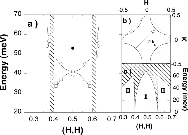
Figure 8: Dispersion of the incommensurate magnetic response for underdoped YBa₂Cu₃O_6.85 along the (110) direction of the magnetic Brillouin zone [92]. The open symbols in a) show the incommensurate spin excitations and the 41 meV resonance mode at the antiferromagnetic wavevector in the odd channel, the full circle shows the 53 meV resonance mode in the even channel. Below 30 meV the magnetic INS intensity is strongly reduced due to a spin-gap. In the hatched region no magnetic spin-excitations are observed. The electron-hole continuum for magnetic spin excitations is shown in c) along the (110) direction for a $d$-wave superconductor with maximal gap of 35 meV. The inset b) shows the wavevector within the fermionic Brillouin zone, for which the spin continuum goes to zero. (From Ref. [92], Copyright ©2004 APS).

As can be seen in a), the magnetic resonance is part of an incommensurate response which extends in energy down to an energy of $\sim 30$ meV (for smaller energies the intensity drops below the background level). In a certain distance from the antiferromagnetic wavevector on either side, the dispersion is interrupted by a momentum region, in which no resonant magnetic spin-excitations are observed. This region, shown as hatched area in Fig. 8, can be identified with the region in which particle-hole-continuum excitations exist. For a $d$-wave superconductor such a region extends all the way down to zero energy, as shown in Fig. 8 c), corresponding to continuum excitations due to node-node scattering. The corresponding wavevector is given by the node-node wavevector, $2k_{N}$, which in superconducting cuprates is slightly displaced from the $(\pi,\pi)$ antiferromagnetic wavevector as can be seen from Fig. 8 b).

In connection with the fact, that the resonance is part of a dispersive spin excitation branch, it is important to realize that the momentum width of the resonance is inhomogeneously broadened as a result of a finite energy window in experiments. Depending on the degree of flatness of the dispersion near the resonance energy the measured momentum width can differ considerably. This is a possible reason why in Bi₂Sr₂CaCu₂O_8+δ the resonance has a much broader momentum width than in YBa₂Cu₃O_6+x.

2.1.10 The spin gap

In fact, the incommensurate excitations are not observed experimentally down to zero energy. Instead, in the low energy region of the incommensurate excitations the INS intensity drops drastically. This ‘spin-gap’ was measured in the superconducting state of La_2-xSr_xCuO₄ [133, 135], where it is of size 3-6 meV, as well as in the superconducting state of YBa₂Cu₃O_6+x. In both systems the spin-gap phenomenon was shown to be sensitive to disorder, with impurities introducing additional states below the spin gap [136, 125]. For La_2-xSr_xCuO₄ it was shown in addition that the spin gap is sensitive to an applied magnetic field in $c$-direction, which also introduces additional states [58].

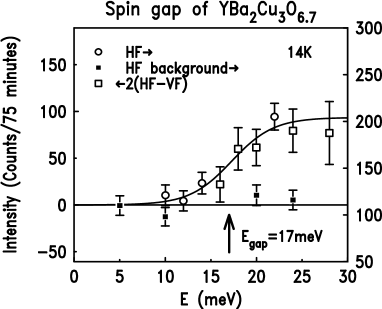
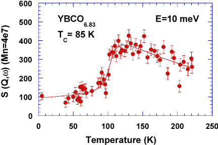
Figure 9: Left: Spin gap in YBa₂Cu₃O_6.7 ($T_{c}=$67 K, $\Omega_{res}=$ 33 meV) at $T=$14 K [109]. Right: Temperature dependence of the INS peak intensity at low energy in YBa₂Cu₃O_6.83 [83]. (From Refs. [109] Copyright ©2000 APS, and [83], Copyright ©1998 Springer).

In Fig. 9, left picture, the spin gap is shown for underdoped YBa₂Cu₃O_6.7, in which case it amounts to 17 meV [109]. In general the spin-gap magnitude follows closely $T_{c}$ according to $E_{sg}=3.8k_{\rm B}T_{c}$ [89]. Only at very low doping it deviates from this linear relation, and shows a smaller spin-gap, e.g. of 5 meV in YBa₂Cu₃O_6.5 [109]. The temperature dependence of the INS intensity at low energy is shown in Fig. 9, right picture. It shows that in underdoped materials the spin-gap persists to temperatures above $T_{c}$.

2.1.11 The spin fluctuation continuum

In addition to the resonance and the dispersive features above and below it, there is also a spin fluctuation continuum, which extends to high energies, see Fig. 8 c. In Fig. 10 the local (wavevector integrated) susceptibility is shown. The continuum extends well above 200 meV.

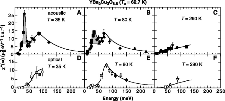
Figure 10: Wavevector integrated frequency dependent magnetic susceptibility for odd (acoustic) and even (optical) modes in underdoped YBa₂Cu₃O_6.6 ($T_{c}$=62.7 K, [106]), for several temperatures. The resonance is shadowed. Below the resonance there are contributions from an incommensurate response, and above the resonance there is a continuum spectrum with a lower threshold of twice the superconducting gap at the Fermi surface points which are connected by a $(\pi,\pi)$ wavevector. (Reprinted with permission from Science, Ref. [106]. Copyright ©1999 AAAS).

The continuum is more clearly visible in the local susceptibility, as it has a much broader momentum width than the resonance feature and the low-energy incommensurate response. The momentum width of the resonance and of the continuum part of the spectrum show different doping dependence. Also, the doping dependence of the total spectral weight is different for the resonance peak and the continuum part of the spectrum. The ratio between the spectral weight of the resonance and the spectral weight of the continuum actually decreases with underdoping, due to a stronger increase of the continuum part of the spectrum [109].

In optimally and overdoped materials the continuum part of the spectrum becomes very small in (energy resolved) intensity and only the resonance part of the spectrum can be observed there. However, because the continuum is spread over a large energy scale, the total (energy integrated) intensity can still be considerable.

2.1.12 Normal state spin susceptibility

In the normal state the spin susceptibility is peaked at the commensurate wavevector ${\bf Q}=(\pi,\pi)$ except for La_2-xSr_xCuO₄ which shows four incommensurate peaks in the normal state. As function of energy, it is peaked around a characteristic frequency $\Omega_{max}$, which decreases with underdoping [81, 100, 137, 83, 84]. An example is shown in Fig. 11 for optimally doped YBa₂Cu₃O_6.92.

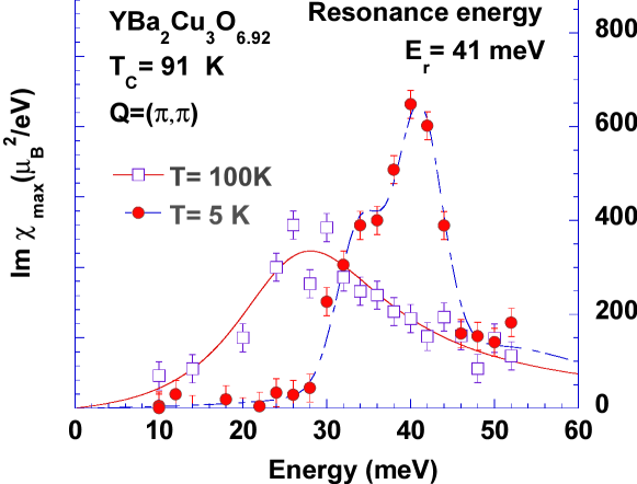
Figure 11: Frequency dependent spin susceptibility at antiferromagnetic wavevector ${\bf Q}=(\pi,\pi)$ in absolute units, for odd (acoustic) excitations in optimally doped YBa₂Cu₃O_6.92 ($T_{c}$=91 K, [138]). Shown are data for the normal state (squares) and for the superconducting state (circles). The normal state susceptibility is characterized by a broad maximum around $\Omega_{max}\sim 30$ meV, that does not coincide with the resonance energy in the superconducting state of $\Omega_{res}\approx 41$ meV. (From Ref. [138] Copyright ©1999 AIP, and [100] Copyright ©1995 Elsevier).

The peak intensity decreases with increasing doping [137, 83, 84]. The overall momentum width of the commensurate response in the normal state was shown to scale with $T_{c}$ [101]. For optimally and overdoped materials the normal state susceptibility at the antiferromagnetic wavevector can be reasonably well described by an overrelaxational form,

$$\chi({\bf Q},\Omega)=\frac{\chi_{{\bf Q}}}{\displaystyle 1-i\;\Omega/\Omega_{max}}.$$ (9)

The spin-fluctuation frequency $\Omega_{max}$ characterizes the normal state response. In the pseudogap state for underdoped cuprates, Eq. (9) is not a good description at low $\Omega\sim E_{sg}$, because of the persistence of the spin-gap. It has been shown that the spin excitation spectrum in the pseudogap state is qualitatively different from that in the superconducting state, showing no resonance feature and a steep incommensurate dispersion with a strongly anisotropic in-plane geometry [139].

2.2 Angle resolved photoemission

Angle resolved photoemission experiments have achieved several important goals in characterizing high-$T_{c}$ materials. First, they showed that a large and well defined Fermi surface exists in these materials. Thus, one can expect that the important fermionic excitations reside near this Fermi surface and thus populate only a small fraction of the phase space. Second, they showed the presence of a shallow extended saddle point in the regions of the Brillouin zone, where the $d$-wave oder parameter is maximal (antinodal regions). Third, it turned out that ARPES spectra near the nodal directions (where the $d$-wave order parameter vanishes) and near the antinodal directions of the Brillouin zone are very different from each other. Near the antinode spectra are dominated by strong self-energy effects, with characteristic $S$-shaped regions in the dispersion and non-trivial line-shapes of the spectra. These self-energy effects persist also away from the antinodes, and continuously evolve into the nodal spectra, which have a simpler line-shape, and where the dispersion anomalies appear in form of kinks. Fourth, the line-widths of the spectra contain important information about the scattering of quasiparticles.

2.2.1 Fermi surface

The existence of a well defined normal state Fermi surface was an object of discussion for some time. The matter is settled in the meanwhile, and a consistent picture has emerged [140, 141]. The existence of a large, hole-like Fermi surface in the normal state was taken as support for the validity of Luttinger’s theorem [142, 143, 144, 145], a conclusion that was confirmed for underdoped, optimally doped and moderately overdoped materials [146]. An example for the quality of experimental Fermi surfaces for Bi₂Sr₂Ca_n-1Cu_nO_2n+4 materials (with $n=1,2,3$ layers per unit cell) is shown in Fig. 12 for different doping levels. The Fermi surface is large and hole-like, showing only slight variations with doping.

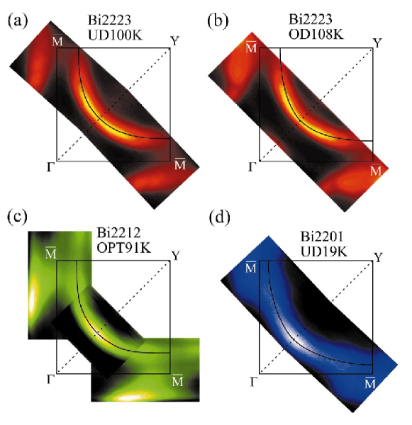
Figure 12: Experimental normal state Fermi surfaces for Bi₂Sr₂Ca_n-1Cu_nO_2n+4 with $n=1,2,3$. (From Ref. [147], Copyright ©2003 APS).

It was found that on the strongly overdoped side of (Bi,Pb)₂(Sr,La)₂CuO_6+δ (Pb-Bi2201) the Fermi surface stays hole-like [148, 149] even when $T_{c}$ is reduced to less than 4 K. For even stronger overdoping ($T_{c}<2$K) a transition to an electron-like Fermi surface was suggested [150, 151]. A similar change of the topology of the Fermi surface was observed in L_2-xSr_xCuO₄ [152, 153, 154], where the transition takes place for $x\approx 0.2$, and the Luttinger sum-rule is fulfilled above and below the transition [153, 154]. Concerning Bi-2212, recent measurements have shown that in heavily overdoped Bi₂Sr₂CaCu₂O_8-δ the bonding Fermi-surface sheet stays hole-like, whereas for the antibonding Fermi-surface sheet a change in the Fermi-surface topology from hole-like to electron-like takes place with increasing doping [155]. The critical doping value was determined as 0.23, corresponding to $T_{c}=55$K. Recently also Tl₂Ba₂CuO_6+δ (Tl2201) was studied in the overdoped range, finding a single large hole-like Fermi-surface for samples with $Tc=63$ K and $T_{c}=30$ K; it was concluded that a topological transition will eventually take place at even higher doping levels for this system as well [156]. The important observation is, that this change in Fermi-surface topology is not accompanied by any abrupt changes in $T_{c}$ as a function of doping. Also, it takes place at a doping level which does not correspond to the extrapolation of the pseudogap crossover line to zero temperature (at doping level 0.19 for Bi2212).

Whereas for overdoped materials the Fermi surface in the normal state is well defined, in optimally and underdoped materials a pseudogap phase exists above the superconducting transition temperature, in which the Fermi surface is present in form of Fermi-surface arcs near the nodal points, separated by gapped antinodal regions [157]. The length of the arcs increases with temperature, until at a characteristic temperature $T^{\ast}$ the arcs join each other and the Fermi surface is restored [157].

2.2.2 Normal-state dispersion and the flat-band region

Typically, for all high-$T_{c}$ cuprates the dispersion of electronic states around the Fermi surface is characterized by the presence of saddle points close to the chemical potential. For simple tetragonal symmetry the corresponding points are the so-called $M$-points in the two-dimensional Brillouin zone, situated at $(0,\pi)$ and $(\pi,0)$ (in units of the inverse lattice constant). To clarify the notation we show in Fig. 13 schematically the behavior of the dispersion in one quarter of the Brillouin zone.

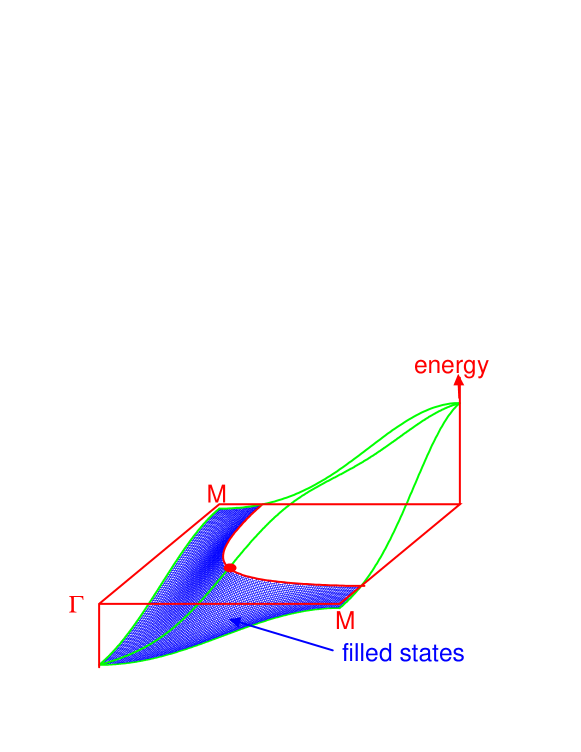
Figure 13: Typical normal state dispersion for a single layered high-$T_{c}$ cuprate shown in one quarter of the Brillouin zone. The filled states are shown as shadowed surface. The Fermi surface is shown as thick curve. At the $M$-points of the Brillouin zone the dispersion has Van Hove singularities very close to the chemical potential. In the superconducting state only the nodal points of the Fermi surface remain, shown as a thick dot in the figure.

Such a dispersion is typical for single layered cuprates. For cuprates with more than one layer per unit cell a splitting of the bands is expected. The case for bilayer compounds, in which a splitting of the Fermi surface into two occurs, will be discussed further below.

The proximity of the van-Hove singularity is seen in Fig. 13 near the points marked ‘$M$’. Also seen as thick dot is the position of the order-parameter node on the Fermi surface, when the material enters a $d$-wave superconducting state. The Fermi velocity in cuprates is of the order of eV$\AA$. This means, that in the vicinity of this node, excitations with energies within the range of $\pm 100$ meV are restricted to a very narrow shell around the Fermi surface. The same is not true for the regions around the $M$-points, as the Van-Hove singularity is within the range of typical excitation energies.

In fact, the dispersion near the $M$-points of the Brillouin zone shows a surprisingly flat behavior in the direction parallel to the Fermi surface [158, 159, 160, 144]. The binding energy of that flat-band region is comparable to the maximal superconducting $d$-wave gap near optimal doping, and increases with underdoping. In the superconducting state the flatness of the dispersion for near-optimally doped materials is even more pronounced. It was suggested [158] that these saddle point singularities may be extended van-Hove singularities in the sense that the quasiparticle mass diverges in one direction, or becomes very large.

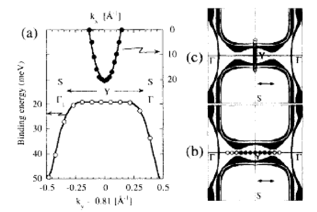
Figure 14: (a) Experimental band dispersion near the van-Hove singularity for untwinned YBa₂Cu₄O₈ ($T_{c}=82$K) at the $Y$-point $(0,\pi)$ of the Brillouin zone. Shown in (b) and (c) are the positions in momentum space where the ARPES spectra were taken. Filled dots correspond to the flat band region. Superimposed is the theoretically calculated Fermi surface projected on the basal plane of the Brillouin zone. (From Ref. [160], Copyright ©1994 APS).

As an example, the dispersion near the saddle points for the compound YBa₂Cu₄O₈ is shown in Fig. 14. In YBa₂Cu₄O₈ the symmetry classification is somewhat different from the case of Bi₂Sr₂CaCu₂O_8-δ, and the saddle point corresponds here to the $Y$ point of the Brillouin zone (see Fig. 14 b,c). From Fig. 14 (a) the flat band region in the direction from the saddle points toward the center of the Brillouin zone is evident. In contrast, the dispersion perpendicular to this is parabolic with Fermi crossings close by.

If not stated otherwise, we will neglect from now on throughout this paper deviations from tetragonal symmetry, which occurs in several high-$T_{c}$ cuprate materials, as these deviations are not important for the understanding of the physics of superconductivity. Accordingly, we use a notation adapted for simple tetragonal symmetry, and commonly used for the system best studied in ARPES, namely Bi₂Sr₂CaCu₂O_8-δ.

From the line-widths of the excitations near the $M$-points one can conclude that scattering is strong between the $M$-point regions. As a result, the flat dispersion at the saddle points is probably a many-body effect, and not a property of the bare electronic structure [141]. Also, for the same reason the flat-band region does not lead to any singularity in the density of states, as there are no sharp quasiparticles present there. However, it can lead to a sizable particle-hole asymmetry.

Finally, for underdoped materials the $M$ point regions stay gapped above the superconducting transition temperature, and these gapped regions are connected by Fermi-surface arcs that grow out of the nodal points of the Brillouin zone [157]. This simultaneous presence of gapped and non-gapped regions leads to the pseudogap-effect.

2.2.3 MDC and EDC

For the experimental study of cuprates it turned out important to consider not only spectra for fixed momentum in the Brillouin zone as function of binding energy (energy distribution curves, EDC), but also spectra for fixed energy as function of momentum along a certain cut in the fermionic Brillouin zone (momentum distribution curves, MDC). The difference is illustrated in Fig. 15 for a typical set of spectra taken on optimally doped Bi₂Sr₂CaCu₂O_8+δ at $T=40$K.

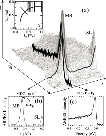
Figure 15: (a) The experimental ARPES intensity as function of binding energy $\omega$ and momentum ${\bf k}$ for optimally doped Bi₂Sr₂CaCu₂O_8+δ at $T=40$K (SL is a superlattice image, MB is the main quasiparticle band). (b) Momentum distribution curves (MDC) from (a). (c) Energy distribution curves (EDC) from (a). The diagonal line in the $\Gamma-Y$ direction of the zone inset, crossing the Fermi surface, shows the corresponding ${\bf k}$ cut. (From Ref. [34], Copyright ©2001 APS).

The corresponding MDC is shown in (b) and the EDC in (c). It is clearly seen that the EDC poses several problems. First, it has a strongly asymmetric line-shape, which does not allow for the determination of the quasiparticle lifetime in a simple way. Instead, the full energy dependent self energy must be extracted in order to characterize quasiparticles. In addition, there is an energy-dependent background at higher energies, which must be subtracted. In contrast, the MDC in panel (b) shows a Lorentzian lineshape (note that MB is the main band; the additional feature, denoted by SL, is due to a superstructure), and the background is rather momentum independent and can easily be subtracted. Also seen in Fig. 15 is that the maxima of the MDC and EDC dispersions at $\omega=0$ and ${\bf k}={\bf k}_{F}$, respectively, do not coincide. Accordingly, it is very important to specify which spectra are used in order to study dispersion anomalies. It turned out that both types of spectra contain important information. In the beginning years of experimental research in the field of cuprates almost exclusively EDC spectra were analyzed. Only in recent years the resolution of experiments became good enough for analyzing MDC’s as well. In Refs. [30, 24, 25] the importance of MDC spectra for comparison with theoretical models was pointed out.

The line shape of the ARPES signal is determined by the spectral function $A(\epsilon,{\bf k})$ (multiplied with the Fermi distribution function). The fact, that the MDC line shape (in contrast to the EDC lineshape) is approximately Lorentzian, can be quantified in terms of a self energy $\Sigma(\epsilon,{\bf k})$ with real part $\Sigma^{\prime}$ and imaginary part $\Sigma^{\prime\prime}$, that in the normal state is related to the spectral function by,

$$A(\epsilon,{\bf k})=\frac{1}{\pi}\;\frac{\Sigma^{\prime\prime}(\epsilon,{\bf k})}{[\epsilon-\xi_{{\bf k}}-\Sigma^{\prime}(\epsilon,{\bf k})]^{2}+[\Sigma^{\prime\prime}(\epsilon,{\bf k})]^{2}\;,}$$ (10)

where $\xi_{{\bf k}}=\epsilon_{{\bf k}}-\mu$ is the bare band-structure dispersion. It is clear from this expression, that the experimental findings are consistent with the notion of a weak momentum dependence and a strong energy dependence of the self energy. Indeed, for momentum independent $\Sigma$ and for $\xi_{{\bf k}}\approx{\bf v}_{F0}({\bf k}-{\bf k}_{F0})$, the MDC is a Lorentzian with a half-width half-maximum (HWHM) of $W_{MDC}=\Sigma^{\prime\prime}(\epsilon)/v_{F0}$ (assuming for simplicity that the MDC-cut is parallel to ${\bf v}_{F0}$).

2.2.4 Bilayer splitting

Bilayer splitting for cuprate superconductors with two conducting layers per unit cell was predicted long ago on theoretical grounds [161, 162], but only in recent years was found in experiments. It is most clearly pronounced in overdoped materials, where it was found first [163, 164].

For dominantly coherent coupling between the planes the appropriate basis is in terms of bonding and antibonding bands. Their dispersion is given in terms of the dispersion for a single layer, $\xi_{{\bf k}}$, by

$$\xi_{\bf k}^{(b)} = \xi_{\bf k}-t_{\perp}({\bf k})$$

$$\xi_{\bf k}^{(a)} = \xi_{\bf k}+t_{\perp}({\bf k})$$ (11)

with an interlayer hopping term $t_{\perp}({\bf k})$. The interlayer hopping has the form [165, 166]

$$t_{\perp}({\bf k})=\frac{1}{4}t_{\perp}\left[\cos(k_{x}a)-\cos(k_{y}a)\right]^{2}\;.$$ (12)

It describes coherent hopping between the CuO₂ planes. Sometimes, a momentum independent incoherent hopping term is added on the right side of Eq. (12).

In Figs. 16 and 17 the main experimental results for the bilayer splitting are shown.

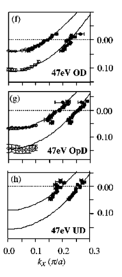
Figure 16: Left: Bilayer-split normal state Fermi surface of heavily overdoped Bi₂Sr₂CaCu₂O_8+δ ($T_{c}$=65 K). (The two weaker features are shadow Fermi surfaces due to superstructure). Solid and dashed lines represent the bonding and antibonding Fermi surfaces, respectively. (From Ref. [167], Copyright ©2002 APS). Right: Normal state dispersion at $k_{y}=1.27\pi$ as a function of $k_{x}$ for Bi₂Sr₂CaCu₂O_8+δ. OD refers to overdoped ($T_{c}$=55 K) at $T=$80 K, OpD to optimally doped ($T_{c}$=91 K) at $T=$100 K, and UD to underdoped ($T_{c}$=78 K) at $T=$100 K. The open circles are peak centroids from EDC’s and the closed circles from MDC’s. The lines are parabolas separated by 70 meV, and shifted with respect to the OD ones by -30 meV for OpD, and by -40 meV for UD. A fit to $\delta\xi({\bf k})=0.5t_{\perp}[\cos(k_{x}a)-\cos(k_{y}a)]^{2}$ gives $t_{\perp}=(57\pm 4)$ meV and a maximum splitting of $114\pm 8$ meV. (From Ref. [168], Copyright ©2004 APS).

First, the bilayer splitting is strongly anisotropic and follows the theoretical predictions [165, 166]. The functional dependence of the bilayer splitting on the momentum, Eq. (12), is experimentally verified [163, 164]. An example for the fit to this functional form is shown on the left in Fig. 17.

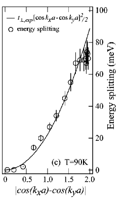
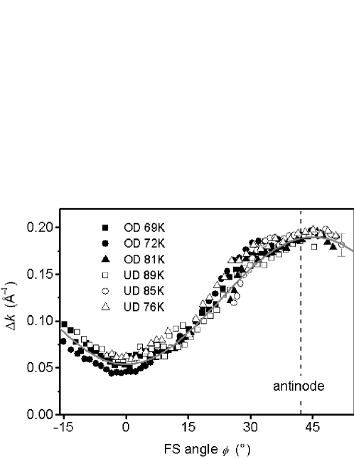
Figure 17: Left: Energy splitting along the antibonding Fermi surface for an overdoped Bi₂Sr₂CaCu₂O_8+δ sample ($T_{c}=$65 K). The curve is $0.5t_{\perp}[\cos(k_{x}a)-\cos(k_{y}a)]^{2}$ with the experimentally determined fitting parameter $t_{\perp}=44\pm 5$ meV. (From Ref. [163], Copyright ©2001 APS). Right: Width of the main Fermi surface, $\Delta k$, versus the Fermi surface angle $\phi$, seen from $(\pi,\pi)$ and measured from the nodal line, for (Bi,Pb)₂Sr₂CaCu₂O_8+δ at several amounts of doping (the $T_{c}$ is indicated). The solid line represents $\Delta k(\phi)=\Delta k_{0}+\Delta k_{1}\sin^{2}(2\phi)$. (From Ref. [146], Copyright ©2002 APS).

According to Eq. (12) the bilayer splitting is zero along the nodal direction $k_{x}=k_{y}$. Near the $M$-point of the Brillouin zone the bilayer splitting is maximal. Recently, it was suggested that a small bilayer splitting of approximately 23 meV remains for Bi₂Sr₂CaCu₂O_8+δ also in nodal direction [169, 171]; furthermore, in YBa₂Cu₃O_6+x a nearly five times larger nodal bilayer splitting has been observed [170].

The second issue refers to the doping dependence of the bilayer splitting. In optimally and underdoped compounds the bilayer splitting was also reported [172, 173, 174, 41], and its magnitude was shown to be independent of doping [172, 168, 170]. As can be seen in Fig. 16, the maximal bilayer splitting amounts to $\approx 114$ meV for all studied values of doping, which suggests a value $t_{\perp}\approx 57$ meV. Thus, with underdoping the bilayer splitting is not lost, but the coherence between the bonding and antibonding bands worsens [175]. The idea, that the bilayer splitting stays constant as a function of doping, is also supported by the observation that the total momentum width of the Fermi surface in the normal state depends strongly on the position on the Fermi surface, but almost not on doping, as illustrated on the right in Fig. 17. This indicates an unresolved bilayer splitting as source for the strong anisotropy of the momentum width for all doping levels, which itself is doping independent [146]. The bilayer splitting in optimally and underdoped materials is of the same order as the linewidth of the quasiparticle excitations, and strong scattering between the bonding and antibonding band can lead to the destruction of coherence between the layers [175]. In this case, the strong mixing between bonding and antibonding band often allows to consider both as a single entity. Assuming as scattering mechanism a spin-fermion interaction this scattering increases with underdoping and is weak in overdoped materials.

2.2.5 Superconducting coherence

First experiments showing particle-hole coherence in the superconducting state were performed by Campuzano et al. [176]. There it was shown that the hole dispersion branch shows a back-bending effect when crossing the Fermi momentum, as expected from BCS theory of superconductivity. Recent improvements in the resolution of ARPES spectroscopy allowed for an impressive experimental verification of particle-hole coherence in the superconducting state including the BCS coherence factors. The main results are reproduced in Fig. 18.

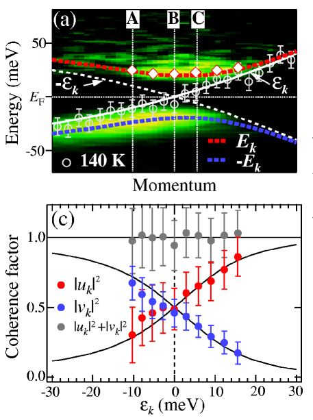
Figure 18: (a) ARPES intensity plot for overdoped Bi₂Sr₂Ca₂Cu₃O_10+δ ($T_{c}$=108 K) in the superconducting state ($T=$60 K). Shown as open white circles is also the dispersion for the normal state ($T=$140 K). The two thick dashed curves are calculated from the BCS spectrum $E_{k}=\sqrt{\epsilon_{k}^{2}+|\Delta_{k}|^{2}}$, where for $\epsilon_{k}$ the white full line is used, and for $|\Delta_{k}|$ the experimental peak energy from 60 K spectra is employed. The white dashed curve shows $-\epsilon_{k}$. (c) shows the coherence factors as experimentally determined from the ARPES intensity (solid circles) compared to the BCS coherence factors derived from the ARPES dispersion (solid lines). (From Ref. [6], Copyright ©2003 APS).

As can be inferred from this figure, the particle-hole mixing is clearly seen in the dispersion both of the hole as well as of the particle branch. The minimum gap between the particle and hole branch is at $k_{F}$, the dispersive features are almost symmetric with respect to $E_{F}$ and both the particle and the hole bands show the typical back-bending effect at $k_{F}$. Matsui et al. [6] also studied the spectral intensity of the two bands as function of ${\bf k}-{\bf k}_{F}$. These weights determine the coherence factors in BCS theory, and they are shown in Fig. 18 (c). The agreement with the BCS theory is striking. The experimental values are very close to

$$|u_{{\bf k}}|^{2}=1-|v_{{\bf k}}|^{2}=\frac{1}{2}\left(1+\frac{\xi_{{\bf k}}}{E_{{\bf k}}}\right)$$ (13)

with $E_{{\bf k}}=\sqrt{\xi_{{\bf k}}^{2}+|\Delta_{{\bf k}}|^{2}}$. Here, $\Delta_{{\bf k}}=\Delta_{0}[\cos(k_{x}a)-\cos(k_{y}a)]/2$ is the $d$-wave gap and $\xi_{{\bf k}}$ is the normal state dispersion which was obtained from the experimental peak positions at 140 K. Note, that the sum of the squares of the coherence factors adds up to one. As $|u_{k}|^{2}$ and $|v_{k}|^{2}$ were determined independently, this condition was not imposed but is an experimental verification of the sum rule $|u_{{\bf k}}|^{2}+|v_{{\bf k}}|^{2}=1$.

This study unambiguously established the Bogoliubov-quasiparticle nature of the sharp superconducting quasiparticle peaks near $(\pi,0)$. It is striking, that in spite of all anomalies observed in high-$T_{c}$ superconductors the superconducting coherence of the quasiparticle peaks is described by these simple BCS formulas.

2.2.6 EDC-derived dispersion anomalies

Important information about the interaction of quasiparticles with collective excitations is obtained by studying anomalous behavior of the quasiparticle dispersion. Such anomalies are due to self-energy effects which arise when quasiparticles couple strongly to collective excitations with finite frequency, leading to inelastic scattering processes. There are two types of experimental dispersions one can study: EDC-derived dispersions and MDC-derived dispersions.

Advances in the momentum resolution of ARPES have led to a detailed mapping of the spectral function in the high $T_{c}$ superconductor Bi₂Sr₂CaCu₂O_8+δ throughout the Brillouin zone [33, 34]. In these first systematic experimental studies of self-energy effects the emphasis was on the EDC-derived dispersions and on the spectral line-shapes as function of energy. The main results of Kaminski et al. [34] are reproduced in Fig. 19. The link of these data to the finite momentum width of the magnetic resonance mode [7, 25] led to a vivid discussion about the fundamental question of what are the relevant low-lying collective excitations that couple to conduction electrons in cuprate superconductors.

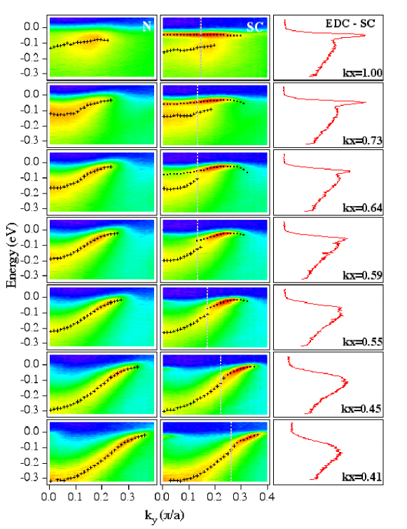
Figure 19: (Left) Normal ($T=$140 K) and (middle) superconducting state ($T=$40 K) ARPES intensity measured on optimally doped Bi₂Sr₂CaCu₂O_8+δ ($T_{c}$=89 K) throughout the Brillouin zone along cuts indicated in the inset of Fig. 15. (Right) superconducting state EDC’s from the momenta indicated by the dashed lines in the middle panels. (From Ref. [34], Copyright ©2001 APS).

On the right column in Fig. 19 superconducting EDC spectra are shown for positions in the Brillouin zone near the Fermi surface, varying from the region near the $M$-point (top spectrum) to the region near the zone diagonal (bottom spectrum), where the node of the $d$-wave order parameter is situated. The spectra near the $M$-point show a characteristic low-energy ‘peak’ and a broader high-energy ‘hump’, separated by a ‘dip’ in the spectrum. The peak and hump-maxima define dispersion branches, that are presented in the middle column as EDC-derived dispersions in the superconducting state. The corresponding normal state EDC dispersions are shown in the left column.

The data indicate a seemingly unrelated effect near the $d$-wave node of the superconducting gap, where the dispersion shows a characteristic ‘kink’ feature: for binding energies less than the kink energy, the spectra exhibit sharp peaks with a weaker dispersion; beyond this, broad peaks with a stronger dispersion [177, 33, 34]. The kink feature near the node is seen both in EDC and MDC derived dispersions. This MDC-derived kink is present at a particular energy all around the Fermi surface [33], and away from the node the dispersion as determined from MDC-derived spectra shows an S-like shape in the vicinity of the kink [30]. The similarity between the excitation energy where the kink is observed and the dip energy at $M$, however, suggests that these effects are related [7].

As seen in Fig. 19, away from the node the kink in the dispersion as determined from EDC spectra develops into a ‘break’; the two resulting branches are separated by an energy gap, and overlap in momentum space. Towards $M$, the break evolves into a pronounced spectral ‘dip’ separating the almost dispersionless quasiparticle branch from the weakly dispersing high energy branch. The kink, break, and dip features all occur at roughly the same energy, independent of position in the zone [34], the kink being at a slightly smaller energy than the break feature [38]. Additionally, the observation that the spectral width for binding energies greater than the kink energy is much broader than that for smaller energies [177, 33, 34] is very similar to the difference in the linewidth between the peak and the hump at the $M$ points.

Another important result comes from the comparison of the dispersions along the $(0,0)\to(0,\pi)$ direction and the $(0,\pi)\to(\pi,\pi)$ direction, which is reproduced in Fig. 20.

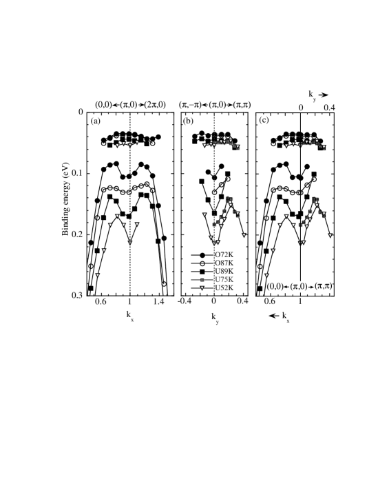
Figure 20: Doping dependence of the dispersion from (a) $(\pi,0)\to(\pi\pm\pi,0)$, (b) $(\pi,0)\to(\pi,\pm\pi)$, and (c) both directions, for the peak and hump in the superconducting state of Bi₂Sr₂CaCu₂O_8+δ. U is underdoped and O is overdoped. (From Ref. [32], Copyright ©1999 APS).

Apart from the increase of the binding energy with underdoping of the high-binding-energy branch one observes a pronounced dispersion minimum also in the direction $(0,0)\to(0,\pi)$. This minimum resembles a mixing between the $(0,\pi)$ and $(\pi,0)$ regions in the Brillouin zone due to scattering, which increases with underdoping.

Finally, the dispersion anomalies were observed also in overdoped materials, taking into account the well resolved bilayer splitting. In this case dispersion anomalies very similar to the ones discussed above, are observed for the bonding band in the antinodal region [163, 36, 178]. These careful experiments show very clearly that for overdoped materials self-energy effects are strong in the antinodal region, however become weak toward the nodal regions. At the nodal point these self-energy effects are unobservable for strongly overdoped materials, whereas other effects, presumably due to electron-phonon scattering, remain observable in the nodal region of the Brillouin zone.

Different experiments focussed on different scattering mechanisms, divided mainly between coupling to phonons and to antiferromagnetic spin fluctuations. Whereas certainly both scattering mechanisms are at work in cuprates, it is of considerable interest to determine the respective coupling constants. For this goal it is important to differentiate between the separate scattering channels. Fortunately this became possible through the careful studies by several groups [38, 36, 178, 39, 40]. These studies are important also from the point of view that they show the intrinsic nature of the dispersion anomalies, which persist even when the bilayer split bands are resolved.

2.2.7 The $S$-shaped MDC-dispersion anomaly

The traditional way of analyzing ARPES data has been that for EDC’s, namely at fixed momentum as a function of binding energy. A much improved precision in momentum space during recent years, however, made it possible to analyze in detail also MDC curves in cuprates, taken at fixed binding energy as a function of momentum [177, 33, 179]. MDC’s have been used in the high temperature cuprate superconductors to study a variety of phenomena, for example as a test for the marginal Fermi liquid hypothesis [179, 37], or to elucidate a dispersion kink along the nodal direction [33], the origin of which was subject of a long debate [34, 49, 38].

In the normal state, it is relatively straightforward to analyze MDC’s, as there is no energy gap complicating the dispersion; the same applies for the superconducting state along the nodal direction [34]. However, qualitative changes occur in the MDC’s due to the energy gap. By analyzing MDC dispersions, one can gain important information on many-body effects in the superconducting state.

             

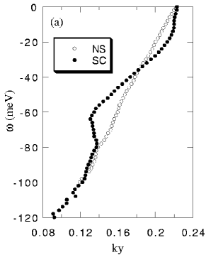
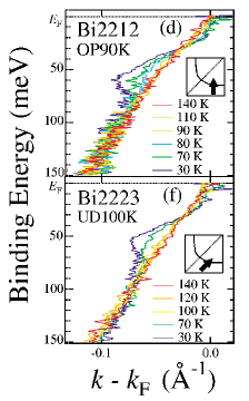
Figure 21: Left: Experimental MDC dispersion in the superconducting state (SC, T=40K) versus that in the normal state (NS, T=140K) of an optimally doped ($T_{c}$=90K) Bi₂Sr₂CaCu₂O_8+δ sample. k_y is in units of $\pi/a$. For this momentum cut, k_x=0.59$\pi/a$. (From Ref. [30], Copyright ©2001 APS). Right: Experimental MDC peak dispersions for Bi2212 (Bi₂Sr₂CaCu₂O_8+δ) and Bi2223 (Bi₂Sr₂Ca₂Cu₃O_10+δ) measured along the cuts indicated in the insets as arrow, for several temperatures from above to below $T_{c}$. The strongest effects correspond to lowest temperatures. (From Ref. [39], Copyright ©2003 APS).

In Fig. 21, MDC dispersions are shown in both the normal and superconducting states roughly midway between the nodal and the antinodal point of the Brillouin zone. The normal state dispersion shows roughly a linear behavior in ${\bf k}$ in the energy range of interest. In the range of 20-60 meV, the superconducting dispersion is also linear, but with a slope approximately half that of the normal state, as noted earlier by Valla et al. [37]. This implies an additional many-body renormalization of the superconducting state dispersion relative to that in the normal state.

Below the gap energy, the MDC derived dispersion shows a completely different behavior when compared with the EDC derived dispersions. The former shows an almost vertical branch toward the chemical potential, whereas the latter shows a backbending from the chemical potential. This effect is, however, easily explained within a BCS picture when taking into account finite lifetime effects of the quasiparticles [30].

Another, more interesting renormalization effect is the $S$-shaped dispersion in the range between 60 and 80 meV, before recovering back to the normal state dispersion at higher binding energies. This $S$-shaped part of the MDC dispersion corresponds to the ‘break’-region in the EDC-derived dispersions, or to the ‘dip’ feature in the EDC’s. Such effects are typical of electrons interacting with a bosonic mode [180, 16], and the mode in the current case has been identified as a spin exciton by some authors [15, 34, 38] and a phonon by others [49]. However, in explaining the effect, one has to bear in mind that the $S$-shaped dispersion anomaly is associated with the superconducting state, which gives an additional restriction for possible interaction mechanisms.

The $S$-shaped regions are observed also when bilayer splitting is resolved, in this case in the bonding band. An example is shown in Fig. 22.

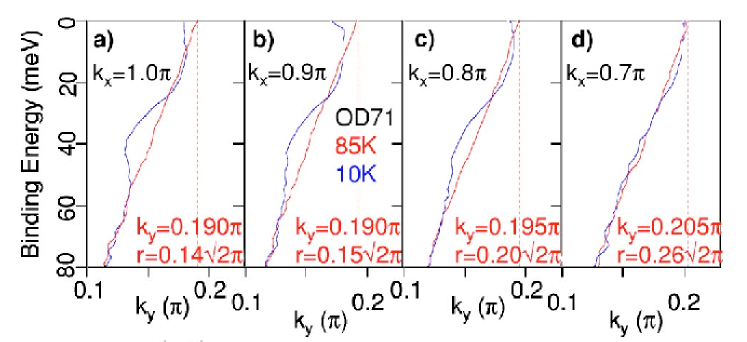
Figure 22: Dependence of the MDC dispersion of the bonding band for an overdoped ($T_{c}=71$ K) Bi₂Sr₂CaCu₂O_8+δ sample on the position in the Brillouin zone. Here, $r$ denotes the radial distance from the $(\pi,0)$ point. The dashed lines mark the Fermi surface crossings. (From Ref. [36], Copyright ©2003 APS).

In this case, for an overdoped sample, however, the degree to which the corresponding effects spread toward the nodal region is smaller than in optimally and underdoped materials.

The $S$-shaped dispersion in the MDC spectra is not observed in nodal direction. Instead, a kink-like feature is present [33, 34, 49, 38, 39], which sharpens in the superconducting state, and this extra sharpening has a temperature dependence similar to that of the antinodal dispersion [38, 40].

2.2.8 The nodal kink

In nodal direction the dispersion is linear in the high-energy and low-energy regions, with different slopes respectively. The two regions are separated by a ‘kink’, which is rather sharp in the superconducting state [179, 33, 34, 49]. This kink is seen both in the EDC and MDC derived dispersion. However, because the MDC width above the kink is rather large, the EDC and MDC derived dispersions differ at high energies.

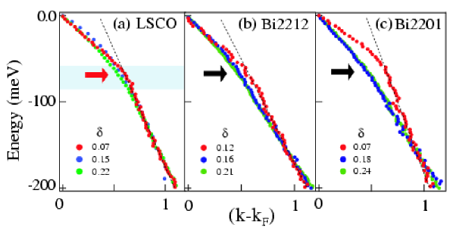
Figure 23: MDC-derived dispersion for La_2-xSr_xCuO₄ (LSCO), Bi₂Sr₂CaCu₂O_8+δ (Bi2212), and Bi₂Sr₂CaCuO_6+δ (Bi2201), for several doping levels as indicated (optimal doping corresponds to $\delta=0.16$), along the nodal ($\Gamma-Y$) direction. Data are taken at 20 K (a,b) and 30 K (c). (From Ref. [140], Copyright ©2003 APS, reprinted by permission from Mcmillan Publishers Ltd: Nature, Ref. [49] Copyright ©2001 NPG).

The nodal kink is seen in a large number of materials with different amounts of doping. As can be seen in Fig.  23, it increases with underdoping and decreases with overdoping. In strongly overdoped samples it is almost absent. As a function of temperature, it is sharp below $T_{c}$ and becomes more rounded in the normal state.

The derivative of the nodal dispersion curve shows a jump at the kink position, and constant parts below and above. These constants define a Fermi velocity $v_{F}$ and a high-energy velocity $v_{HE}$.

2.2.9 Fermi velocity

Experimentally, because the dispersion of the EDC maxima and the MDC maxima differ from each other, it is important to specify how the Fermi velocity is extracted from the data. Clearly, the picture is complicated by a strong energy dependence of self-energy effects. Here the fact helps, that self-energy effects are weakly momentum dependent. Thus, although the line shape of the EDC’s is highly non-trivial both at anti-nodal as well as at nodal points, the shape of the MDSs is very well approximated by a Lorentzian. From Eq. (10) one can see that the velocity at binding energy $\epsilon$ is given by,

$${\bf v}(\epsilon)=\frac{\displaystyle{\bf v}_{0}(\epsilon)+\partial_{{\bf k}}\Sigma^{\prime}(\epsilon,\hat{\bf k})}{\displaystyle 1-\partial_{\epsilon}\Sigma^{\prime}(\epsilon,\hat{\bf k})},$$ (14)

where $\hat{\bf k}$ is the position of the MDC maximum, and it was assumed that the momentum variation of $\Sigma^{\prime\prime}$ is negligible. Assuming that (away from the saddle point) the bare velocity is a constant in the energy region of interest, ${\bf v}_{0}(\epsilon)\equiv{\bf v}_{F0}$, and taking into account that the momentum dependence of the self energy is weak (this follows from the fact that the MDC spectra are Lorentzian), then one can neglect the energy dependence of $\partial_{{\bf k}}\Sigma^{\prime}(\epsilon,\hat{\bf k})$ and the main energy dependence comes from the renormalization factor $Z(\epsilon,{\bf k})=1-\partial_{\epsilon}\Sigma^{\prime}(\epsilon,{\bf k})$. It is clear that the ratio between the velocities $v_{HE}$ and $v_{F}$ in Fig. 24 gives directly the ratio between the quasiparticle renormalization factor $Z=Z(0,{\bf k}_{F})$ and a high energy renormalization $Z_{HE}(\epsilon)$, which is only weakly energy dependent [181].

The Fermi velocity near the nodal point is large and of the order of 1.8 eV$\AA$ [34, 182] and virtually doping independent [182]; weak systematic changes with doping are e.g. in YBa₂Cu₃O_6+x within 0.2 eV$\AA$ [170]. This is in contrast to the slope of the dispersion above roughly 70 meV, which changes strongly with doping and amounts to 2.5-5.5 eV$\AA$ [38, 182, 170]. In Fig. 24 the two velocities are shown for several cuprates as function of doping.

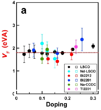
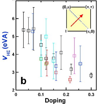
Figure 24: Normal state quasiparticle velocity along the nodal direction, obtained from momentum-distribution curves, for various cuprates as function of doping. The high energy dispersion is separated by a kink at about 70 meV from the low energy dispersion with different slope. Accordingly, the velocities differ for the low-energy region and the high-energy region. (a) Low energy (determined from 0-50 meV) Fermi velocity and (b) high energy (determined from 100-200 meV) velocity. (Reprinted by permission from Mcmillan Publishers Ltd: Nature, Ref. [182] Copyright ©2001 NPG).

The angular dependence of the Fermi velocity $v_{F}$ along the Fermi surface is shown in Fig. 25. It is rather isotropic in the normal state, however is renormalized differently in the superconducting state, leading to an anisotropy along the Fermi surface. From Fig. 25 one can see that the Fermi velocity is reduced near the $(\pi,0)$ points of the Brillouin zone, however only slightly so near the nodes.

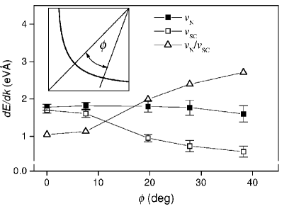
Figure 25: Fermi velocities for optimally doped Bi₂Sr₂CaCu₂O_8+δ ($T_{c}=$91 K) in normal (solid squares) and superconducting (open squares) state as function of Fermi surface angle $\phi$ defined in the inset. The ratio between normal state and superconducting state Fermi velocities is also shown as open triangles. (From Ref. [37], Copyright ©2000 APS).

It is interesting to note, that the higher energy part of the nodal dispersion is linear to highest measured energies [183], and does not extrapolate to the Fermi crossing [33, 49]. This suggests, that the high energy dispersion is strongly renormalized and cannot be described by simple models assuming a fixed bandwidth as function of doping. Certainly, the whole band structure changes with doping, and it is the low energy part which stays surprisingly stable from the overdoped to underdoped materials. This is reflected in the constance of the Fermi velocity shown in Fig. 24 (a), in the weak change of the Fermi surface, and in the pinning of the saddle point singularity at the $M$ points to the low-energy region, within about 100 meV near the chemical potential. The strong renormalization of the high-energy part of the spectrum lets us conclude, that if the continuum part of a bosonic spectrum that couples to electrons is responsible for these renormalizations, then this bosonic spectrum must extend to high ($\sim$eV) energies.

Finally, an estimate of the bare Fermi velocity can be obtained by comparing the MDC and EDC widths of the spectra (assuming a definite energy dependence of the self energy in the vicinity of the Fermi surface, and a Lorentzian MDC lineshape). In Ref. [155] the bare Fermi velocity was determined for optimally doped Bi₂Sr₂CaCu₂O_8+δ, and was shown to vary from 4 eV$\AA$ at the node to 2 eV$\AA$ at the antinode. This is consistent with Ref. [184], which found a nodal bare Fermi velocity of 3.4 eV$\AA$ in optimally doped Bi(La)-2201 ($T_{c}=32$K), of 3.8 eV$\AA$ in underdoped Bi(Pb)-2212 ($T_{c}=77$K), and of 3.9 eV$\AA$ in overdoped doped Bi(Pb)-2212 ($T_{c}=75$K).

2.2.10 Spectral lineshape

It has been known for some time that near the $(\pi,0)$ point of the zone, the spectral function in the superconducting state of Bi₂Sr₂CaCu₂O_8+δ shows an anomalous lineshape, the so called ‘peak-dip-hump’ structure [4, 185, 186, 15]. This structure was also found in YBa₂Cu₃O_7-δ [187], and in Bi₂Sr₂Ca₂Cu₃O_10+δ [188, 149].

Extensive studies on Bi₂Sr₂CaCu₂O_8+δ as a function of temperature revealed that this characteristic shape of the spectral function is closely related to the superconducting state. In the normal state, the ARPES spectral function is broadened strongly in energy, the broadening increasing with underdoping [186]. When lowering the temperature below $T_{c}$, a coherent quasiparticle peak grows at the position of the leading edge gap, and the incoherent spectral weight is redistributed to higher energy, giving rise to a dip and hump structure [4, 185, 15]. This peak-dip-hump structure is most strongly developed near the $M$-point of the Brillouin zone. Below $T_{c}$, the spectral peak quickly narrows with decreasing temperature [189], and sharp quasiparticle peaks were identified well below $T_{c}$ along the entire Fermi surface [177].

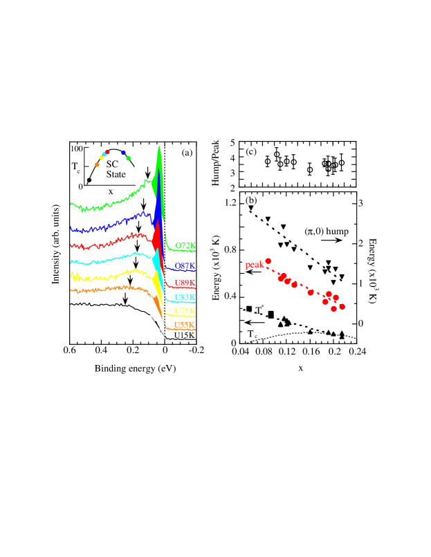
Figure 26: (a) Doping dependence of experimental ARPES spectra at the ($\pi,0$) point for Bi₂Sr₂CaCu₂O_8+δ from overdoped (O) to underdoped (U) at $T=15$K. The inset shows the corresponding values for $T_{c}$. The quasiparticle coherent weight is indicated by shadowing and decreases with underdoping. (b) Doping dependence of the pseudogap temperature scale $T^{\ast}$, the quasiparticle peak binding energy, the binding energy of the hump feature, denoted by an arrow in (a), and the ratio of the latter two in (c). (From Ref. [32], Copyright ©1999 APS).

The doping dependence of the spectral lineshape was carefully studied by Campuzano et al. [32]. In Fig. 26 it is seen that the peak loses weight with underdoping. The peak, dip, and hump feature all move to higher binding energy with underdoping.

The well defined quasiparticle peaks at low energies contrast to the high energy spectra, which show a broad linewidth which grows linearly in energy [179, 190]. This implies that a scattering channel present in the normal state becomes gapped in the superconducting state [191]. The high energy excitations then stay broadened, since they involve scattering events above the threshold energy. While this explains the existence of sharp quasiparticle peaks, a gap in the bosonic spectrum which mediates electron interactions leads only to a weak dip-like feature [192]. This suggests that the dip feature is instead due to the interaction of electrons with a sharp (in energy) bosonic mode. The sharpness implies a strong self-energy effect at an energy equal to the mode energy plus the quasiparticle peak energy, giving rise to a spectral dip [16]. The fact that the effects are strongest at the $M$ points implies a mode momentum close to the $(\pi,\pi)$ wavevector [14].

The non-trivial spectral line-shape is further complicated due to the presence of bilayer splitting. In this case the different behavior of matrix elements as function of the photon energy for bonding and antibonding bands has to be used in order to separate the effects. It was found, that the peak-dip-hump structure is also present when the bilayer splitting is resolved. Two examples are shown in Fig. 27.

Figure 27: Left: ARPES spectrum for an overdoped Bi₂Sr₂CaCu₂O_8+δ sample ($T_{c}=$ 65 K) at the point $(0.11,1)\pi$ of the Brillouin zone as function of energy (in eV), measured at $T=10$ K. The cross refers to the antibonding peak and the bar to the bonding peak. An experimental fitting procedure assigns the high-energy hump mainly to the bonding spectral function, as seen from the three fitting curves shown for the bonding, the antibonding, and the total spectrum. (From Ref. [163], Copyright ©2001 APS). Right: Bonding band and antibonding band ARPES spectrum for a (Bi,Pb)₂Sr₂CaCu₂O_8+δ sample at the $(\pi,0)$ point of the Brillouin zone measured at $T=20$ K. Here, the bonding and antibonding contributions have been separated by varying the photon energy $h\nu$. (From Ref. [193], Copyright ©2006 APS).

In Fig. 27 (left), the bonding band shows a pronounced dip in the spectrum near the bonding band Fermi momentum. Consequently, there are strong self-energy effects present even in such overdoped materials. The same Figure also reveals that the self-energy effect in the antibonding band is much weaker. In Fig. 27 (right), the difference in the spectral line-shapes between bonding and antibonding band spectra is shown at the $(\pi,0)$ point of the Brillouin zone, revealing again a stronger dip feature in the bonding spectrum. This characteristic asymmetry between bonding and antibonding line-shapes has been an important information for the assignment of the effect to the interaction of quasiparticles with the spin-1 resonance mode [24, 193].

2.2.11 The antinodal quasiparticle peak

The antinodal quasiparticle peak (or coherence peak) in the superconducting state determines the spectral gap. With underdoping, the sharp quasiparticle peak moves to higher binding energy, indicating that the gap increases [32]. The quasiparticle peak has also been traced as a function of Fermi surface angle, and has been found consistent with a $d$-wave symmetry of the order parameter [4, 194, 195]. The $d$-wave symmetry of the superconducting order parameter was unambiguously demonstrated by phase sensitive tests (see [196]).

In Fig. 28, data for the gap-anisotropy as determined from ARPES experiments are shown for several doping levels.

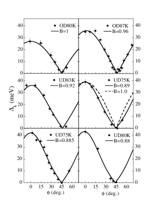
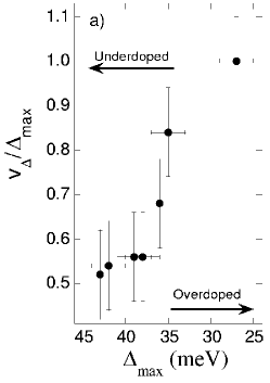
Figure 28: Left: Superconducting gap as function of Fermi surface angle $\phi$ for a series of (Bi,Pb)₂Sr₂CaCu₂O_8+δ samples with varying doping. The fits use a functional form $\Delta_{k}=\Delta_{\rm max}[B\cos(2\phi)+(1-B)\cos(6\phi)]$. The dashed line shows for comparison the function $\Delta_{\rm max}\cos(2\phi)$. (From Ref. [123]). Middle: Normalized slope of the gap at the node ($v_{\Delta}/\Delta_{\rm max}$) vs gap maximum $\Delta_{\rm max}$. (From Ref. [123], Copyright ©1999 APS). Right: The ratio between the nodal order parameter, defined by the formula $\Delta_{k}=\Delta_{\rm v}\cos(2\phi)$ in such a way that the slopes $v_{\Delta}$ coincides with the measured one. Open circles are directly from experimental $v_{\Delta}$ (middle panel), full circles are obtained by using the $v_{\Delta}$ from the fitted curves in the left picture.

The magnitude of the gap is clearly consistent with a $d_{x^{2}-y^{2}}$-wave symmetry of the order parameter. In optimally doped materials the magnitude of the gap follows very closely a cos$(2\phi)$-dependence on the Fermi surface angle [186],

$$\Delta_{{\bf k}}=\frac{1}{2}\Delta_{M}\left[\cos(k_{x}a)-\cos(k_{y}a)\right]$$ (15)

which takes its maximal value $\Delta_{M}$ closest to the $M$ point of the Brillouin zone. Whereas the same holds also for overdoped materials, in underdoped materials deviations from this simple behavior have been detected [123, 174]. Interestingly, toward underdoping the slope of the order parameter along the Fermi surface at the nodal point decreases, although the maximal gap at the antinodal point increases (this is in contrast to what is deduced from, e.g., thermal conductivity measurements [197]). As shown in Fig. 28 (right), the ratio between this slope and the transition temperature stays roughly constant. This is what one would expect for a BCS superconductor. In strong contrast, the ratio of the maximal gap to the transition temperature sharply rises with underdoping. This might be an indication that in underdoped cuprates an additional order parameter is present near the antinodes. This idea is supported by the experimental fact that in the pseudogap phase the antinodal regions stay gapped, whereas the nodal regions show well defined Fermi surface pieces.

Borisenko et al. [174] have measured the gap separately for the bonding and antibonding bands and have found, that for underdoped Bi(Pb)₂Sr₂CaCu₂O_8-δ ($T_{c}=$ 77 K) each of the bilayer split bands supports in the superconducting state a gap of the same magnitude. The consequences become clear when transforming the order parameters from plane representation to bonding-antibonding representation,

$$\Delta_{\parallel}({\bf k}) = \frac{\Delta^{(a)}_{{\bf k}}+\Delta^{(b)}_{{\bf k}}}{2},$$ (16)

$$\Delta_{\perp}({\bf k}) = \frac{\Delta^{(a)}_{{\bf k}}-\Delta^{(b)}_{{\bf k}})}{2}.$$ (17)

The apparent experimental finding, that

$$\Delta^{(a)}_{{\bf k}}=\Delta^{(b)}_{{\bf k}},$$ (18)

means that the interplane pairing interaction $V_{\perp}$ vanishes.

Apart from the binding energy of the quasiparticle peak its spectral weight is of interest. In Fig. 29 the temperature evolution of the spectral weight is reproduced for optimally doped Bi₂Sr₂CaCu₂O_8+δ.

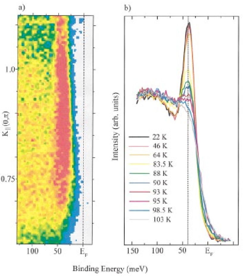
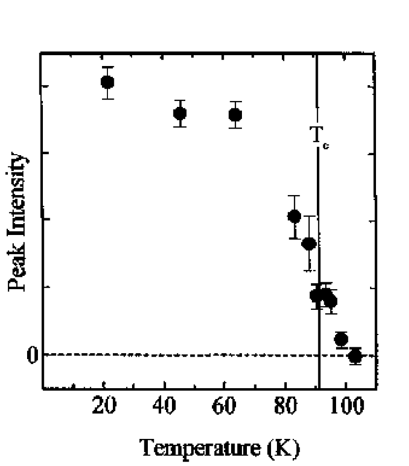
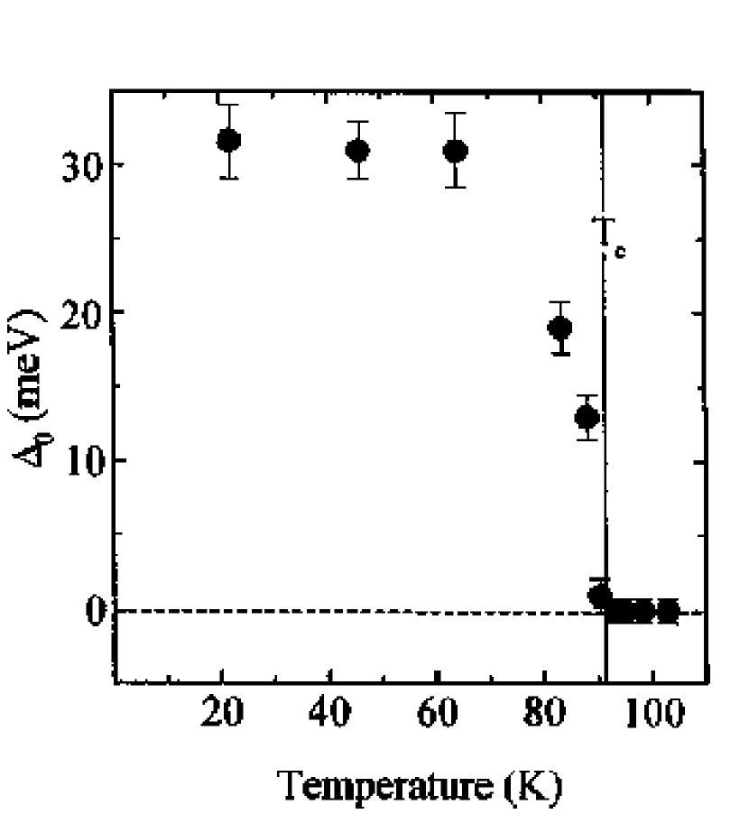
Figure 29: (a) Spectral density plot in $\Gamma M$ direction for an optimally doped Bi₂Sr₂CaCu₂O_8+δ sample ($T_{c}$=91 K) at $T=46$K. The superconducting peak intensity is seen as dispersionless feature of high intensity between $\sim 25\ldots 50$ meV binding energy. (b) Spectra integrated over the region in (a) as function of temperature. The strongest peak intensity is observed at lowest temperatures. On the right the peak intensity and the gap $\Delta_{0}$ are shown as function of temperature. (From Ref. [198], Copyright ©1999 APS).

The weight follows an order parameter like behavior, and becomes very small in the normal state. It was argued [189] that using a different modeling of the spectral lineshape, the peak broadens drastically when entering the normal state, instead of a reduction of the peak weight. The analysis in Fig. 29 uses a phenomenological model to fit the peak and the remaining part of the spectrum separately, in order to extract the peak weight.

The spectral weight $z_{A}$ of the peak as a function of doping is discussed in Fig. 30.

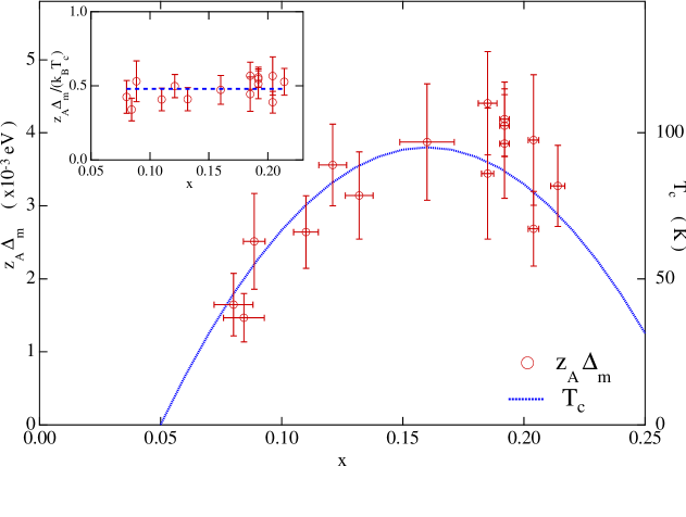
Figure 30: Doping dependence of $z_{A}\Delta_{m}$ (open circles) at $(\pi,0)$ in comparison with $T_{c}$. Here, $z_{A}$ is the low-temperature coherent weight and $\Delta_{m}$ the maximum gap obtained from the position of the quasiparticle peak. The inset shows the ratio $z_{A}\Delta_{m}/(k_{B}T_{c})$. All data are at $T=$14 K. (From Ref. [199], Copyright ©2001 APS).

A drop of the peak weight with underdoping was also analyzed in Refs. [32, 200] and can be seen directly in Fig. 26. The quantity $z\Delta_{M}/k_{B}T_{c}$ stays roughly constant as function of doping, as seen in the inset in Fig. 30 [199]. Also, the hump moves to higher binding energy and loses weight with underdoping [32]. This doping evolution of the quasiparticle peak points to an increasing mode intensity at the $(\pi,\pi)$ wavevector with underdoping. Again, there is a similarity to the nodal direction: the low energy renormalization of the dispersion below the kink energy increases with underdoping [38], consistent with a common origin of both effects.

2.2.12 The spectral dip feature

If one assumes that the spectral-dip feature is due to coupling of quasiparticles to a sharp bosonic mode, then one can determine the mode energy from the ARPES spectra. The energy of the bosonic mode, as inferred from the energy separation $\Omega_{0}$ between the peak and the dip, was shown to decrease with underdoping [32]. As was shown in theoretical studies [16, 7, 25] it is the position of the spectral dip with respect to the quasiparticle peak which determines the characteristic frequency of self-energy effects. The position of the hump feature does not contain as much reliable informations about the self energy. The doping variation of the peak-dip separation is shown in Fig.31, where for comparison also the mode frequencies of the magnetic resonance mode as inferred from INS experiments are plotted. The agreement is striking.

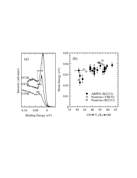
Figure 31: (a) ARPES-spectra for Bi₂Sr₂CaCu₂O_8+δ at $(\pi,0)$ for different amounts of doping, showing the determination of the peak-dip separation. (b) Doping dependence of the mode energy inferred from ARPES, and from INS [83, 201, 99]. (From Ref. [32], Copyright ©1999 APS).

In fact, as inferred from tunneling experiments, the peak-dip separation also decreases with overdoping, so that it follows roughly the superconducting transition temperature [44]. Similarly, the kink energy is maximal at optimal doping and decreases both with underdoping and overdoping [38], indicating some relationship between the kink at the nodal $N$ point and the peak-dip-hump structure at the $M$ point.

2.2.13 Real part of self energy: renormalization of dispersion

The most direct test for the interaction of quasiparticles with bosonic modes comes from the recent achievement of the direct determination of the real part of the self energy. This determination is based on the fact that the dispersion of the MDC maxima $\hat{\bf k}$ is determined from Eq. (10) as

$$\epsilon-\xi_{\hat{\bf k}}-\Sigma^{\prime}(\epsilon,\hat{\bf k})=0,$$ (19)

where $\xi_{{\bf k}}$ is the bare dispersion, and $\Sigma^{\prime}(\epsilon,\hat{\bf k})$ the real part of the self energy at the MDC maximum. It was assumed here that $\Sigma^{\prime\prime}(\epsilon)$ is not momentum dependent in the region where the MDC-Lorentzian is peaked (see later). There are two ways to proceed from here. One either determines the bare dispersion independently (see e.g. Ref. [184]), or one subtracts from Eq. (19) the corresponding equation for the normal state. Assuming a linear bare dispersion and neglecting the momentum variation of $\Sigma^{\prime}(\epsilon,\hat{\bf k})$ for $\hat{\bf k}$ varying between $\hat{\bf k}_{N}$ and $\hat{\bf k}_{SC}$, where (N) refers to the normal and (SC) to the superconducting state, one obtains

$${\bf v}_{F0}(\hat{\bf k}_{N}-\hat{\bf k}_{SC})\approx\Sigma_{SC}^{\prime}(\epsilon,\hat{\bf k})-\Sigma_{N}^{\prime}(\epsilon,\hat{\bf k}).$$ (20)

Using the former technique Johnson et al. [38] have studied the self-energy effects in the nodal direction for several doping values. As seen in Fig. 32, in addition to some interactions present already in the normal state (most probably due to the spin-fluctuation continuum and due to electron-phonon interaction), there are clearly self-energy effects which set in at the superconducting transition temperature. These self-energy effects show an order-parameter-like temperature dependence, very similar to the intensity of the resonance mode observed in INS experiments. This effect can be assigned to the coupling with the magnetic resonance mode. Note, that by no means that exhausts all self-energy effects in the nodal direction. It is well established that electron-phonon interaction is present in cuprate systems, and they lead to additional contributions to the real part of the self energy [49, 51]. However, these contributions develop smoothly through $T_{c}$, in contrast to the effects discussed in Ref. [38].

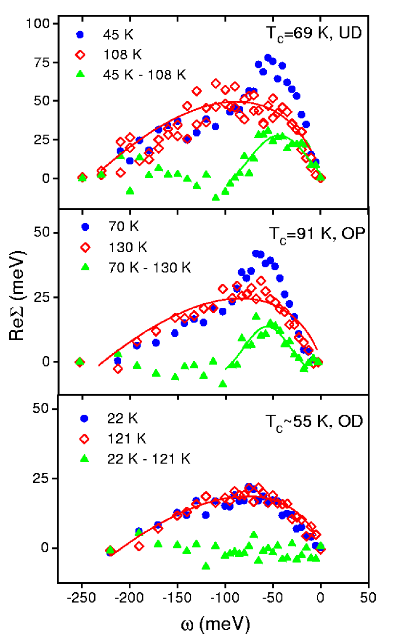
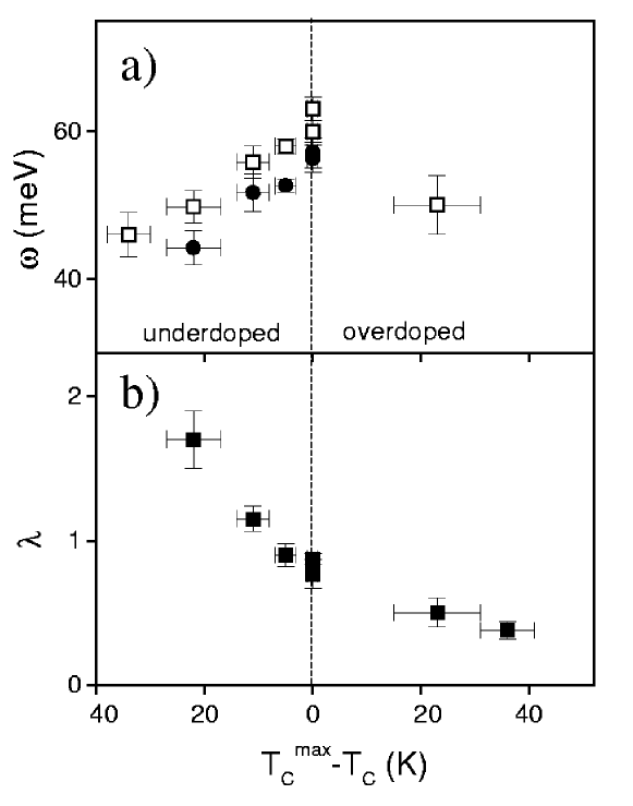
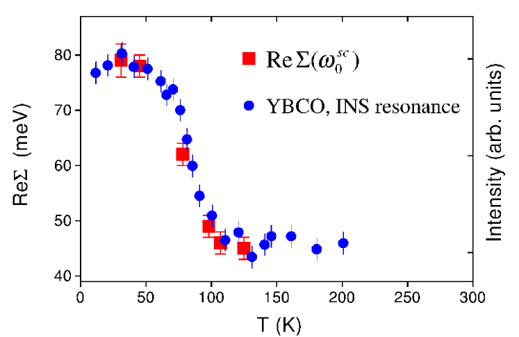
Figure 32: Left: Re $\Sigma(\omega)$ as function of binding energy for superconducting (full dots) and normal state (open diamonds) for an overdoped ($T_{c}$=55 K), optimally doped ($T_{c}$=91 K), and underdoped ($T_{c}$=69 K) Bi₂Sr₂CaCu₂O_8+δ sample taken in nodal direction. The difference between superconducting and normal Re $\Sigma(\omega)$ is shown as triangles. The peak in this quantity defines the peak energy $\omega_{0}^{sc}$. Right: at the top the energy $\omega_{0}$ of the maximum value of Re $\Sigma(\omega)$ in the superconducting state, and $\omega_{0}^{sc}$ are shown as function of doping. The middle panel shows the coupling constant $\lambda=(\partial\mbox{Re}\Sigma/\partial\omega)_{E_{F}}$. In the bottom panel the temperature dependence of Re $\Sigma(\omega)$ in nodal direction is shown for the underdoped sample, together with the intensity of the resonance mode observed in INS studies of underdoped YBa₂Cu₃O_6+x ($T_{c}=74$ K, [106]). (From Ref. [38], Copyright ©2001 APS).

It is clear from this study, that the self-energy effects in the nodal region due to the resonance mode play no role for the overdoped materials. In Fig. 32 this can be seen from the lower left panel. The nodal coupling constant, shown in Fig. 32 (b), is in the overdoped region due to other effects. However, the steep rise as a function of temperature when entering the superconducting state, that is present in the optimally doped and underdoped region, is consistent with an interaction with the magnetic resonance mode, which sets in at the superconducting transition temperature.

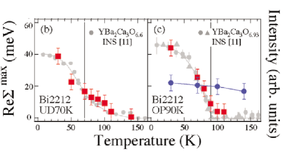
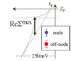
Figure 33: Maximum value of Re $\Sigma(\omega)$ as function of temperature measured along an off-nodal cut for underdoped ($T_{c}=$ 70 K) and optimally doped ($T_{c}=$ 90 K) Bi₂Sr₂CaCu₂O_8+δ. The off-nodal cut is performed about midway between the nodal and antinodal points. For comparison, also points for a nodal cut are shown for the optimally doped case (circles). The intensity of a resonance peak of YBa₂Cu₃O_6+x with similar $T_{c}$ is superposed. (From Ref. [39], Copyright ©2003 APS).

A similar picture is obtained for off-nodal cuts, as shown in Fig. 33 [39]. The magnitude of Re $\Sigma$, determined as shown schematically on the right in Fig. 33, is shown as function of temperature superimposed with the INS data. The magnitude of the self-energy effects here even more clearly traces the intensity of the resonance mode, both for underdoped and optimally doped materials. It was also shown, that corresponding effects in single layered compounds are weak [39].

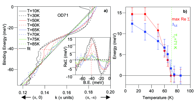
Figure 34: (a) MDC dispersion for an overdoped Bi₂Sr₂CaCu₂O_8+δ ($T_{c}=$71 K) sample, along $(\pi,0)-(\pi,\pi)$ for several temperatures. The inset shows the temperature dependence of Re $\Sigma$. The strongest effect is observed at lowest temperatures. (b) Temperature dependence of the maximum in Re $\Sigma$ (circles) and the superconducting leading edge gap $\Delta_{LE}$ (squares). (From Ref. [36], Copyright ©2003 APS).

Gromko et al. [36] have refined the studies of self-energy effects near the antinodal point of the Brillouin zone by resolving separately bonding and antibonding bands. An example is shown in Fig. 34 (left), where for an overdoped Bi₂Sr₂CaCu₂O_8+δ sample clearly an $S$-shaped MDC dispersion has been observed near the $(\pi,0)$ point in the bonding band when entering the superconducting state. In contrast, in the normal state this self-energy effect is absent, as can be seen from the temperature variation of the effect shown in Fig 34. This is a convincing prove that self-energy effects near the $(\pi,0)$ point of the Brillouin zone, that are due to interactions of quasiparticles with some sharp mode, are clearly observed in addition to bilayer splitting effects. The temperature behavior of the real part of the self energy is shown on the right hand side of Fig 34. As can be seen, the temperature behavior follows an order parameter like behavior. Furthermore, as the experiment was performed on an overdoped sample, this shows that although for overdoped materials the nodal renormalization due to the resonance mode vanishes, this is not so for the antinodal point. The range for which the interaction with the resonance mode is relevant is shown in Fig. 35. Clearly, for overdoped compounds there are renormalizations present in the antinodal region, however these do not extend to the nodal point. It is for optimally and underdoped materials, that the range of interaction also includes the nodal point.

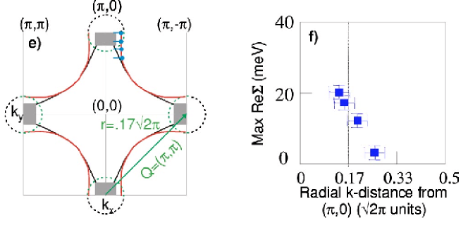
Figure 35: Experimentally deduced self-energy effects for an overdoped Bi₂Sr₂CaCu₂O_8+δ ($T_{c}=$71 K) sample, analyzed for the bonding band. The locations of the MDC cuts are indicated in the Brillouin zone on the left hand side. The circles denote the locus, where Re$\Sigma$ decays to half its maximal value at $(\pi,0)$. The real part of the self energy Re$\Sigma$ as a function of distance from the $(\pi,0)$ point, $r$, is shown in the right panel. The order parameter node corresponds to $r=0.5$. (From Ref. [36], Copyright ©2003 APS).

In a study by Kim et al. [42] the coupling strength parameter for quasiparticles with binding energy $\Delta_{M}$ at the antinodal point, defined as

$$\lambda_{\Delta}=\frac{\Sigma^{\prime}(-\Delta_{M},{\bf k}_{M})}{\Delta_{M}},$$ (21)

was studied both in the bonding and antibonding bands of (Pb,Bi)₂Sr₂CaCu₂O_8+δ with various doping levels (the momentum dependence of $\Sigma^{\prime}$ can be neglected in the region between the Fermi crossings nearest to the $M$ point). It was found, that $\lambda_{\Delta}$ increases with underdoping [41]. It reaches very large values of approximately 8 for $p\approx 0.12$ ($T_{c}=77$ K), and for overdoped samples with $p\approx 0.21$ ($T_{c}=69$ K) still is approximately 3 [42]. Note in this regard, that the gap $\Delta_{M}$ itself increases with underdoping, and consequently $\lambda_{\Delta}$ tests the real part of the self energy at an increasing binding energy with decreasing doping level. A similar analysis in the normal state yielded a doping independent value for the coupling strength of around 1. In the nodal direction, where the gap vanishes, the analogous quantity

$$\lambda_{N}=-\lim_{\epsilon\to 0}\frac{\Sigma^{\prime}(\epsilon,{\bf k}_{N})}{\epsilon},$$ (22)

(where ${\bf k}_{N}$ is the nodal wavevector) was found to be about 1 for the normal state, with additional self-energy effects in the superconducting state [43].

2.2.14 Imaginary part of self energy: quasiparticles lifetime

Interesting information can be obtained also from the linewidth of the MDC spectra, which is directly connected to the imaginary part of the self energy, or to the scattering rate of the quasiparticles. From Eq. (10) it is seen, that under the assumption that the momentum variation of the imaginary part of the self energy $\Sigma^{\prime\prime}(\epsilon,{\bf k})$ can be neglected in the region in which the Lorentzian is peaked, the MDC half-width half-maximum in direction of ${\bf v}_{F0}$, $W_{MDC}$, is given by,

$$W_{MDC}=\frac{\Sigma^{\prime\prime}(\epsilon,{\bf k})}{v_{F0}}.$$ (23)

An analysis of the momentum width of the quasiparticles moving in nodal direction as function of binding energy was performed by Valla et al. [179]. In Fig. 36 the EDC’s along the nodal direction are shown on the left. It was found that the EDC spectra, scaled to the same peak position, coincide.

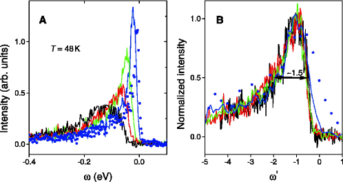
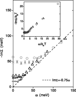
Figure 36: (A) EDC’s for optimally doped Bi₂Sr₂CaCu₂O_8+δ, obtained in the $(0,0)\to(\pi,\pi)$ direction (after subtracting a background). (B) EDC’s scaled to the same peak position showing that the overall shape scales linearly with binding energy. The peak width is approximately 1.5 times the binding energy. Right: Im $\Sigma$ obtained from MDC peak widths (solid symbols) and from EDC peak widths (open symbols) as a function of binding energy for temperatures of 48 K (diamonds), 90 K (triangles), and 300 K (circles). Inset: same data plotted in dimensionless units confirming scaling behavior. (Reprinted with permission from Science, Ref. [179]. Copyright ©1999 AAAS).

This corresponds to a scaling relation $A(\omega)=A(E_{p})f(\omega/E_{p})$ with $\omega$ the electronic energy, and $E_{p}$ the peak position of the EDC. The energy width of the quasiparticle peak, $W_{EDC}$ is proportional to the binding energy, $W_{EDC}(E_{p})\approx 1.5E_{p}$ [142, 179]. The corresponding data for Im $\Sigma$ extracted from the EDC spectra is shown in Fig. 36 on the right for several temperatures. All data approach for high energies the asymptotics Im $\Sigma\approx-0.75\omega$ independent of temperature. For a given temperature, Im $\Sigma$ is constant up to energy $\omega\approx 2.5k_{B}T$. The inset demonstrates a scaling behavior for the nodal direction,

$$\mbox{Im}\Sigma(\omega,T)=k_{B}T\cdot F(\frac{\omega}{k_{B}T})\;,$$ (24)

where $F$ is a scaling function. This behavior resembles that of the marginal Fermi liquid hypothesis of Varma et al. [202, 192].

Recently Kaminski et al. scrutinized the momentum dependence of this effect in the normal state. When going away from the nodal direction, there is an additional temperature independent term. They found that the imaginary part of the self energy above $T_{c}$ in the intermediate energy region ($2.5k_{B}T{{}_{\textstyle<}\atop{\textstyle\sim}}\omega{{}_{\textstyle<}\atop{\textstyle\sim}}200$ meV) can be written as

$$\mbox{Im}\Sigma({\bf k}_{F},\omega)=a({\bf k}_{F})+b\omega,$$ (25)

where the coefficient $b$ is isotropic for both optimally doped and overdoped materials. In contrast, the coefficient $a$ is strongly momentum dependent for underdoped and optimally doped compounds, its anisotropy following the behavior of the pseudogap along the Fermi surface. That means, it is zero on a Fermi surface arc around the node, and increases to about 10 times the pseudogap at the antinodes. For strongly overdoped samples without a pseudogap the coefficient $a$ is isotropic as well. In Fig. 37 the variation of the coefficients $a$ and $b$ around the Fermi surface are shown for optimally doped Bi₂Sr₂CaCu₂O_8+δ.

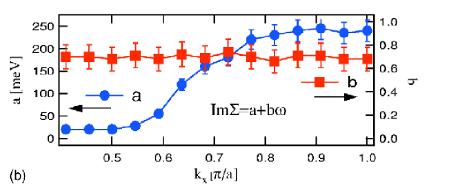
Figure 37: Variation of the coefficients $a$ and $b$ in the equation Im$\Sigma({\bf k}_{F},\omega)=a({\bf k}_{F})+b\omega$ around the Fermi surface for optimally doped Bi₂Sr₂CaCu₂O_8+δ above $T_{c}$. (From Ref. [155], Copyright ©2005 APS).

In the superconducting state, it was argued recently that the MDC peak width in near-nodal direction, when resolving nodal bilayer splitting, shows at low binding energies ($|\omega|{{}_{\textstyle<}\atop{\textstyle\sim}}75$ meV) a superposition of an $\omega$ and an $\omega^{3}$ behavior [171]. This would be consistent with theoretical predictions of Refs. [203, 204]. Above $\sim 75$ meV a nearly linear dependence of the MDC peak width on binding energy is recovered, that is almost unaffected by the superconducting transition [171].

Turning to temperature dependence, Valla et al. [179] have reported an MDC linewidth growing linearly with temperature in the range $T_{c}<T{{}_{\textstyle<}\atop{\textstyle\sim}}300$ K. In Fig. 38 the momentum widths are shown as function of temperature for different positions on the Fermi surface.

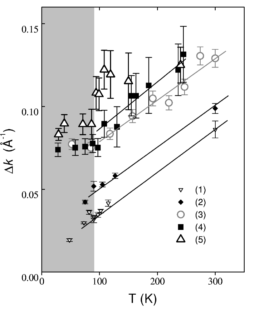
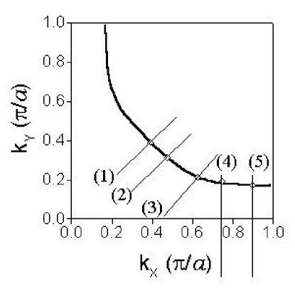
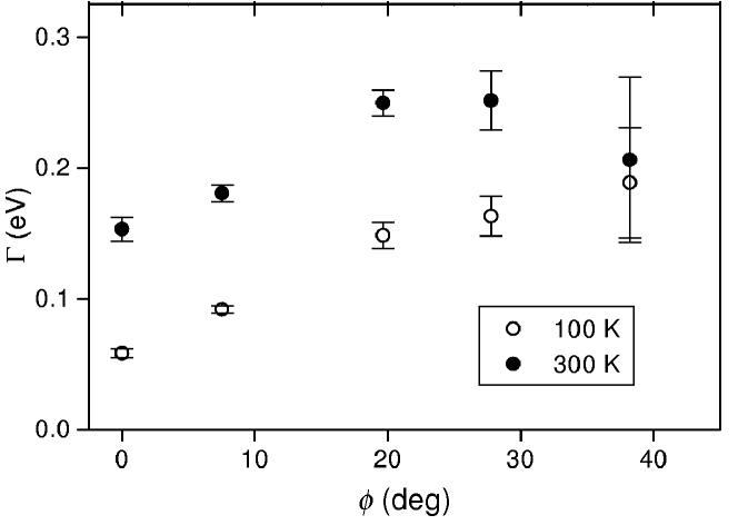
Figure 38: Normal state momentum widths as a function of temperature for different positions on the Fermi surface (indicated in the top right picture) obtained by fitting the MDC’s with Lorentzian lineshapes. Widths are measured at the Fermi level and at the leading edge, in the normal and in superconducting (gray region) state, respectively. The dependence as function of position on the Fermi surface is shown in the right lower picture ($\phi$ is measured from the nodal direction). (From Ref. [37], Copyright ©2000 APS).

The temperature dependence is linear for most of the Fermi surface with a slope independent on the $k_{F}$ position. However, the temperature independent offset varies along the Fermi surface. As a consequence, the imaginary part of the self energy (or the ‘scattering rate’) at the peak positions around the Fermi surface follows the behavior

$$\mbox{Im}\Sigma({\bf k}_{F},T)=a^{\prime}({\bf k}_{F})+b^{\prime}k_{B}T$$ (26)

with a momentum independent constant $b^{\prime}$ and a temperature-independent constant $a^{\prime}({\bf k}_{F})$. As can be inferred from the extrapolation $T\to 0$ in Fig. 38, for the nodal direction, $a^{\prime}({\bf k}_{N})\approx 0$ holds [37]. The scattering rate, given by the product of the momentum width and the normal state Fermi velocity, is shown as a function of the Fermi surface angle in the lower right panel of Fig. 38. It can be seen that the scattering rate for fixed temperature increases away from the nodal point of the Fermi surface, revealing the variation of $a^{\prime}({\bf k}_{F})$ along the Fermi surface.

In the superconducting state the functional dependence on the binding energy is modified in the low-energy region, and the MDC peak width in the nodal Fermi surface point ($\omega=0$) of the bonding state in optimally doped Bi₂Sr₂CaCu₂O_8+δ was fitted to a $T^{3}$ functional dependence [171].

In summary, the normal state scattering rate depends for $\omega\ll k_{B}T$ linearly on temperature, but is independent of frequency, and for $\omega\gg k_{B}T$ is linearly depending on frequency, but temperature independent. In both cases the linearity coefficients are isotropic around the Fermi surface, and there is an energy- and temperature independent but anisotropic term which vanishes in nodal direction. Again both these findings are consistent with the marginal Fermi liquid hypothesis [202]. For intermediate energies, however, $\omega\sim k_{B}T,\Delta_{{\bf k}}$ there are additional effects beyond the marginal-Fermi-liquid phenomenology present.

For example, in the superconducting state there are additional features and clear deviations from the linearity of the scattering rate as a function of binding energy. Generally, for large binding energies the behavior linear in $\omega$ still is present. However, recent studies of the nodal linewidths as function of energy [40, 171] revealed that at moderate energies there is a ‘kink effect’ in Im $\Sigma$, in accordance with the finding in the real part of the self energy by Johnson et al. [38, 171]. This is illustrated in Fig. 39.

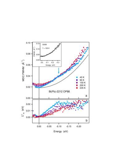
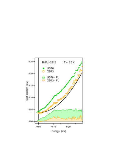
Figure 39: Temperature and doping dependence of self-energy effects for nodal quasiparticles determined from the full width at half maximum of the momentum distribution curves. Left: temperature dependence for optimally doped Bi(Pb)₂Sr₂CaCu₂O_8+δ; the contribution from a highly overdoped sample ($T_{c}=69$K) at 130 K (inset and gray line) is subtracted to obtain the imaginary part of the self energy (using FWHM/2 times $v_{F}=4$ eV $\AA$). Right: doping dependence of the corresponding curves; shown are data for an underdoped ($T_{c}=76$K) and an overdoped ($T_{c}=73$K) sample at 25 K. (From Ref. [40], Copyright ©2004 APS).

The effect is absent for highly overdoped ($T_{c}=$69 K) compounds, however clearly visible for overdoped Bi₂Sr₂CaCu₂O_8+δ with $T_{c}=$73 K, optimally doped Bi₂Sr₂CaCu₂O_8+δ and for underdoped Bi₂Sr₂CaCu₂O_8+δ ($T_{c}=$76 K). As seen from Fig. 39 (b), the kink in Im $\Sigma$ vanishes above $T_{c}$. Also shown in this figure is a comparison between an overdoped and an underdoped sample, showing that underdoped materials exhibit a much stronger kink effect that overdoped materials. This is consistent with the behavior of the real part of the self energy in nodal direction, shown in Fig. 32 [38]. The doping and temperature dependence of the sudden change in the MDC linewidths shown in Fig. 39 is consistent with the doping and temperature dependence of the intensity of the magnetic resonance mode observed in INS.

In summary, for the nodal direction, the combined information from the experimental analysis of effects both in Re$\Sigma$ and Im$\Sigma$ is, that the resonance mode has sizable contributions to nodal quasiparticle scattering for underdoped, optimally doped, and slightly overdoped materials. This is consistent with the scenario for the nodal self-energy effects proposed in [7]. For strongly overdoped materials its contribution to nodal quasiparticle scattering is negligible. Furthermore, for a momentum region around the antinodal direction the data are consistent with a coupling to the spin-fluctuation spectrum even when the overdoping is so strong that the nodal effects due to the magnetic resonance mode are unobservable. This finding is consistent with the apparent decrease in intensity of the magnetic resonance mode with overdoping. The already weaker nodal effect disappears earlier than the antinodal one when overdoping the material.

2.2.15 Isotope effect

Recently the isotope effect on the dispersion spectra has been studied [54] and it was found that it shows a complicated behavior, shown in Fig. 40. The shift is small in the low-energy region, with the isotope effect on the gap value being small and random between different samples in both magnitude and sign, regardless of the isotope mass [54]. Thus, it can be assumed that the low-energy region of the dispersion is only weakly affected by the isotope exchange.

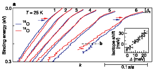
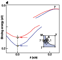
Figure 40: Isotope induced changes of the dispersion along the cuts shown in the inset of (d), for optimally doped Bi₂Sr₂CaCu₂O_8-δ with different oxygen isotopes at $T=25$K. In (a) the MDC-derived dispersions are shown for cuts starting from nodal direction 1. The dispersions are shifted in k-direction for convenience. The inset shows the isotope shift near 220 meV binding energy as a function of the superconducting gap of the same MDC. In (d) the EDC-derived dispersion for cut 7 is shown. (Reprinted by permission from Mcmillan Publishers Ltd: Nature, Ref. [54] Copyright ©2001 NPG).

On the other hand, the high-energy dispersion shows a sample-independent, reproducible and reversible isotope effect that is strongly anisotropic and becomes small in the normal state. The isotope shift changes sign when going from the nodal direction to the antinodal direction, as is shown in the inset of Fig. 40 (a).

However, the strength of the self-energy effects at low binding energies seems to be independent on the isotope mass. This can be seen also from Fig. 40, where neither the low binding energy slopes nor the size of the break in panel (d) change considerably, although the overall dispersion is modified by a renormalization factor. This renormalization affects the dispersion, but does not seem to affect the value of the gap. This is also consistent with the negligible change in $T_{c}$ from 92 K to 91 K upon isotope substitution ¹⁶O $\to$ ¹⁸O. It seems, that the effect of phonons is to contribute to an overall renormalization of the dispersion, although the superconducting properties are only weakly affected.

2.2.16 Relation to pseudogap phase

Finally, there is important information contained in the doping dependence of the self-energy effects. In underdoped compounds, there is a pseudogap between $T_{c}$ and $T^{\ast}$ [205, 186]; the pseudogap is maximal near the $M$-point of the Brillouin zone and is zero at arcs centered at the $N$-points which increase with temperature [157]. In the pseudogap state above $T_{c}$, there are low energy renormalizations in the dispersion, and some trace of the kink feature persists. But in the the work by Johnson et al. [38], it was clearly shown that an additional renormalization of the dispersion sets in just at $T_{c}$. This indicates that the bosonic spectrum redistributes its spectral weight when entering the superconducting state. The additional low energy renormalization of the dispersion below the kink energy follows an order parameter like behavior as a function of temperature [38]. Arguing that the renormalization near the nodal region for underdoped materials is influenced by the coupling to the same bosonic mode which causes the strong self-energy effects at the $M$ point of the Brillouin zone, the above implies that some mode intensity may be present in the pseudogap state already, but there is an abrupt increase in the mode intensity when going from the pseudogap state into the superconducting state, and this increase shows an order parameter like behavior as a function of temperature below $T_{c}$.

2.3 C-axis tunneling spectroscopy

Unusual spectral dip features in tunneling data of Bi₂Sr₂CaCu₂O_8-δ are found in point contact junctions [206], in scanning tunneling spectroscopy (STM) [207, 208, 209], in break junctions [210, 208, 44, 211], and in intrinsic c-axis tunnel junctions [212]. A consistent picture emerged from all these different tunneling techniques [211]. These data show a peak feature, usually assigned to the maximal $d$-wave superconducting gap, and a hump feature at higher bias, separated from the peak by a pronounced dip feature. SIN junctions usually show a spectrum strongly asymmetric around the chemical potential. In many SIN data, also the self-energy effects appear stronger on the occupied side of the spectrum [206, 207, 208]. Recently, however, Zasadzinski et al. [213] reanalyzed STM data by Hudson et al. [209] and argued that after subtracting a background the resulting tunneling spectra are rather symmetric. The issue is unsolved and needs further investigation. The dip feature has been observed in tunneling spectra of the single Cu-O₂ layer compound Tl₂Ba₂CuO₆ as well [214], where it appears weaker. Interestingly, also INS data show that a weak resonant magnetic excitation exists in that material [108].

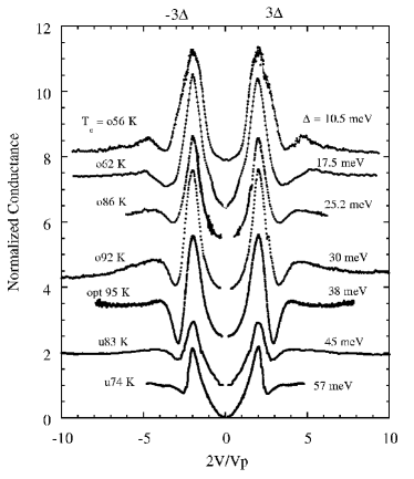
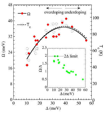
Figure 41: Left: SIS tunneling conductances of Bi₂Sr₂CaCu₂O_8-δ for various amounts of hole-doping from overdoped (o) via optimally doped (opt) to underdoped (u). The voltage has been scaled in units of $\Delta$. The curves have been shifted for clarity. Right: Dependence of the dip-peak energy separation $\Omega$ as function of the spectral gap energy $\Delta$ determined from the c-axis tunneling spectra on Bi₂Sr₂CaCu₂O_8-δ. $\Omega$ follows $T_{c}$, not $\Delta$. The inset shows that the ratio $\Omega/\Delta$ never exceeds 2. (From Ref. [44], Copyright ©2001 APS).

In order to extract information about the bosonic mode which would produce a dip feature in the tunneling conductance, a systematic study as a function of doping was performed in break junction tunneling spectroscopy by Zasadzinski et al. [44]. There, the doping dependence in Bi₂Sr₂CaCu₂O_8-δ of the peak-dip-hump structure was determined over a wide range of doping. Corresponding spectra are reproduced in Fig. 41 (left panel). It was found that the dip-peak energy separation, $\Omega$, follows $T_{c}$ as $\Omega=4.9k_{B}T_{c}$, as demonstrated in the right panel of Fig. 41. In the inset one can see that, as expected for an excitonic mode, $\Omega$ approaches but never exceeds $2\Delta$ in the overdoped region, and $\Omega/\Delta$ monotonically decreases as doping decreases and the superconducting gap increases. The dip feature is found to be strongest near optimal doping. Similar shifts of the dip position with overdoping were reported previously by STM [215]. Together with the ARPES results, these studies give a detailed picture about the doping dependence of the mode energy involved in electron interactions in the superconducting state.

2.4 Optical spectroscopy

Self energy effects can also be studied by optical spectroscopy assuming some model for the optical response. A common way is to write the complex optical conductivity in terms of an optical single-particle self-energy $\Sigma^{op}$ as

$$\sigma(\omega)=\frac{i}{4\pi}\;\frac{\omega_{pl}^{2}}{\omega-2\Sigma^{op}(\omega)}$$ (27)

with the plasma frequency $\omega_{pl}$, that can be determined experimentally from the absorption spectra in the near-infrared region [45]. The imaginary part of the self energy determines an energy dependent carrier scattering rate via

$$\mbox{Im}\Sigma^{op}(\omega)=-\frac{1}{2\tau(\omega)}.$$ (28)

Using the above model, Hwang et al. [45] studied the self-energy effects for different doping levels and temperatures in Bi₂Sr₂CaCu₂O_8-δ. They found that the optical single-particle self-energy shows a sharp feature which weakens with doping and cannot be resolved anymore beyond a doping level of 0.23 holes per copper atom.

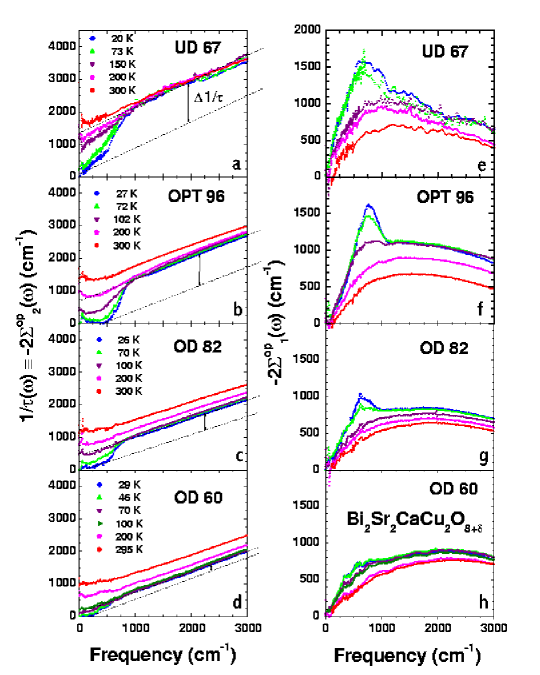
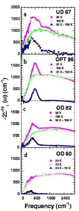
Figure 42: The optical self energy for different doping levels of Bi₂Sr₂CaCu₂O_8-δ, with the imaginary part in the left column, and the real part in the middle column. The feature due to the magnetic resonance can be seen as peak in the difference spectrum between superconducting state and normal state of the real part of the optical self energy, shown in the right column. (Reprinted by permission from Mcmillan Publishers Ltd: Nature, Ref. [45] Copyright ©2001 NPG).

As can be seen in Fig. 42, the imaginary part of $\Sigma^{op}$ shows a linear in $\omega$ behavior at high frequencies, consistent with what is obtained by ARPES spectroscopy. This high-frequency scattering rate generally decreases with increasing doping. In the superconducting state there is a sharp onset of scattering at a finite frequency, seen on the left in Fig. 42, which in the real part of the self energy leads to a sharp peak, shown in the middle row of Fig. 42. This sharp peak is restricted to the superconducting state, and a study of the doping and temperature dependence allowed the authors of Ref. [45] to assign this “optical resonance mode effect” to the interaction of quasiparticles with the magnetic resonance mode. This is demonstrated on the right in Fig. 42, where the difference of the real part of the self energy between the superconducting and the normal state is shown. The frequency position of the peak in the real part of the optical self energy is consistent with the frequency position of the peak in the real part of the self energy obtained from ARPES spectroscopy along the nodal direction, shown in Fig. 32. Also consistent with these latter data, the amplitude of the peak on Re$\Sigma^{op}$ decreases with doping. The study of the optical self energy also shows that a weak effect of the magnetic resonance mode is still observed for overdoped Bi₂Sr₂CaCu₂O_8-δ with $T_{c}=$ 82 K and 60 K. The optical studies of [45] add support to the picture emerging from the ARPES studies.

Optical data along the $a$-axis of a detwinned single crystal of YBa₂Cu₃O_6.50 (underdoped, $T_{c}=59$ K) confirmed this picture and added further support for a correlation between the effects observed in these data and the spin-1 magnetic resonance observed in inelastic neutron scattering [216]. As in the case for Bi₂Sr₂CaCu₂O_8-δ a peak in the data for $-2\Sigma^{op}_{1}(\omega,T)$ is present that sharpens in the superconducting state. The temperature dependence of the peak magnitude follows closely the intensity of the magnetic resonance mode [216].

An issue of discussion [217, 218] referred to the non-observability of the optical self-energy effect due to coupling to the magnetic resonance mode for doping values beyond $p=0.23$ [45]. This claim was based on the extrapolation of the measured data to higher doping levels. However, one has to bear in mind that the optical self energy is a quantity which is not resolved with respect to the position on the Fermi surface, in contrast to ARPES. Thus, it is well possible that self-energy effects persist to the highest doping levels, but are too weak to be observed by optical spectroscopy. This is also consistent with the finding, that the region around the $M$ point in which strong self-energy effects due to coupling to the resonance mode occurs, shrinks with doping, and consequently contributes less and less to the averaged self energy.

Another method which proofed to be very useful to extract information about the interaction of the electrons with a bosonic mode from the optical data was suggested by Marsiglio et al. [219]. It is based on the function

$$W(\omega)=\frac{1}{2\pi}\frac{{\rm d}^{2}}{{\rm d}\omega^{2}}\frac{\omega}{\tau(\omega)}.$$ (29)

In Fig. 43 results of this function extracted from experimental optical scattering rates are shown for optimally doped materials.

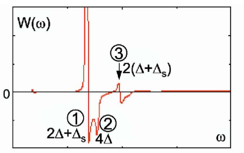
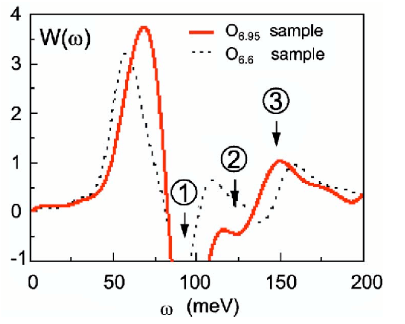
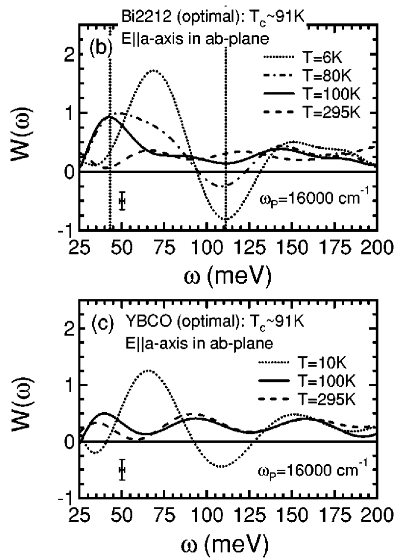
Figure 43: Left: The lower part of the picture shows the function $W(\omega)=(2\pi)^{-1}\partial^{2}_{\omega}[\omega/\tau(\omega)]$ obtained from experimental $a$-axis optical scattering rate data for an optimally doped YBa₂Cu₃O_6.95 untwinned single crystal (full line) and for an underdoped untwinned YBa₂Cu₃O_6.6 single crystal (dashed line). (Reprinted by permission from Mcmillan Publishers Ltd: Nature, Ref. [220] Copyright ©2001 NPG). In the upper part the assignment of the structures to characteristic frequencies obtained from the theory of Abanov et al. [21] are shown for comparison. $\Delta$ is the maximal superconducting $d$-wave gap, $\Delta_{s}$ is the frequency of a sharp bosonic peak coupled to electrons (from Ref. [21], Copyright ©2001 APS). Right: The same experimental functions $W(\omega)$ obtained for optimally doped Bi₂Sr₂CaCu₂O_8+δ (top) and for untwinned optimally doped YBa₂Cu₃O_6.95 for several temperatures (from Ref. [222], Copyright ©2002 APS).

Carbotte et al. [220] analyzed an optimally doped untwinned YBa₂Cu₃O_6.6 single crystal. The strong maximum in $W(\omega)$ was theoretically shown to be at $\Delta+\Delta_{s}$, where $\Delta$ is the superconducting gap and $\Delta_{s}$ the frequency of a sharp bosonic mode assumed to be coupled to electrons. Furthermore, Abanov et al. [21] assigned additional features, denoted in Fig. 43 (left) with 1,2 and 3, to the three characteristic frequencies $2\Delta+\Delta_{s}$, $4\Delta$ and $2(\Delta+\Delta_{s})$. In a detailled recent study by Cásek et al. [221] the assignments of the maximum at $\Delta+\Delta_{s}$ (at low temperatures) and the minimum at $2\Delta+\Delta_{s}$ have been confirmed, however noticeable contributions of quasiparticles away from the antinodal regions of the Brillouin zone have been found to complicate the interpretation, in particular for the remaining extrema.

As can be seen in the lower left picture of Fig. 43, the $\Delta+\Delta_{s}$-peak corresponds to 69 meV, the $2\Delta+\Delta_{s}$-minimum to 100 meV, the $4\Delta$-minimum to 130 meV, and the $2\Delta+2\Delta_{s}$-peak to 150 meV. This is consistent with $\Delta\approx 30$ meV and $\Delta_{s}\approx 40$ meV [21]. Tu et al. found from optical data for optimally doped Bi₂Sr₂CaCu₂O_8+δ the values $\Delta=34\pm 3$ meV and $\Delta_{s}=40\pm 3$ meV [222]. For optimally doped YBa₂Cu₃O_6.95 the same procedure gave $\Delta=30\pm 4$ meV and $\Delta_{s}=40\pm 4$ meV [222, 223]. The corresponding curves $W(\omega)$ are shown in Fig. 43 (right) (the feature at $4\Delta$ is not resolved here). These values are in excellent agreement with the gap values obtained by ARPES and tunneling experiments, and with the mode frequency of the magnetic resonance mode observed in INS. Finally, as can be seen from Fig. 43 (right), in the normal state this characteristic structure is not present. This is consistent with the assumption that in the normal state the mode contribution is not present.

3 The collective mode as spin-1 exciton

3.1 Theoretical models

There are several theoretical interpretations of the resonance mode observed in the magnetic INS signal. In all theories the resonance mode is an excited pair of quasiparticles with total lattice momentum ${\bf Q}=(\pi/a,\pi/a)$ and spin $S=1$ [224, 225, 226, 227]. Lavagna and Stemman [228], and Abrikosov [229] give an interpretation in terms of a van Hove singularity in the Stoner continuum. Demler and Zhang [230] proposed within the SO(5) approach an interpretation in terms of an antibound state in the particle-particle channel ($\pi$-resonance or $\pi$-particle, [230, 231, 226]). This interpretation was, however, shown to be in conflict with the experimental finding that the resonance always appears below twice the maximum $d$-wave gap in the superconducting state [224, 232]. Vojta et al. [233] gave an interpretation as a soft mode directly related to the nearby antiferromagnetically ordered state. Herbut and Lee [234] considered within QED₃-theory the effect that vortex fluctuations have on the spin dynamics and give an interpretation of the resonance as four overlapping collective particle-hole modes of the phase fluctuating $d$-wave superconducting state, centered at the node-node wavevectors. An interpretation in terms of a roton-like excitation, appearing as a coupled mode in the spin- and charge response (‘hybrid spin-charge roton’) was suggested by Uemura [235, 236].

Studies of the spin-excitation spectrum for a striped ground state (exhibiting stripe like modulations of charge and spin) have been performed in Refs. [237, 238, 239, 240, 241, 242, 243, 244]. Striped states have been employed to describe in particular the spin excitation spectrum in La_2-xSr_xCuO₄. However, so far this picture has not been as successful in describing YBa₂Cu₃O_7-δ and Bi₂Sr₂CaCu₂O_8+δ.

Finally, a promising candidate is the interpretation as a bound state (spin exciton) in the particle-hole channel. Here, a number of techniques have been applied, including slave-particle approaches within the $t-J$ and Hubbard models [245, 246, 247, 248, 249, 224, 225, 250, 251, 252, 253], Hubbard-operator techniques for the $t-t^{\prime}-J$ model [254, 255, 256], memory-function approaches within the $t-J$ model [257, 258] BCS models in random phase approximation (RPA) [260, 261, 262, 263, 264, 134], FLEX-approximations in the Hubbard model [265, 13, 266, 29], or spin-fermion models [267, 17, 268, 269]. Theories based on such ‘spin-exciton models’ have been especially successful in reproducing in detail the experimentally determined spin-excitation spectra in YBa₂Cu₃O_7-δ and Bi₂Sr₂CaCu₂O_8+δ. With some modifications of the model also the low-energy spectrum in La_2-xSr_xCuO₄ has been described [270]. Detailled quantitative predictions for the energy- and momentum-dependent spectra determined experimentally have been obtained to date only within the spin-exciton models. The following discussion will concentrate on a review of results obtained with those.

Although differing in the doping dependence of the band structure and exchange coupling, most of the above-mentioned models for the spin-1 exciton ultimately determine the magnetic susceptibility for a given fixed doping value by a relation of the form

$$\chi(\omega,{\bf q})=\frac{\chi_{0}(\omega,{\bf q})}{1-J_{{\bf q}}\chi_{0}(\omega,{\bf q})}\;.$$ (30)

The parameter $J_{{\bf q}}$ can for example be interpreted as a Hubbard $U$, an exchange constant $J$, or a spin-fermion coupling $\bar{g}$, depending on the model and on the form of the susceptibility $\chi_{0}$ which is used. A common form for $J_{{\bf q}}$ is (from now on we use units in which $a=1$),

$$J_{\bf q}=J_{0}-2J\left[\cos(q_{x})+\cos(q_{y})\right],$$ (31)

which includes an onsite term $J_{0}$ and an effective exchange interaction $J$ that is restricted to nearest neighbors. This restriction is generally assumed to be a very good approximation in cuprates. The ‘bare’ irreducible susceptibility $\chi_{0}(\omega,{\bf Q})$, is determined as [63]

$$\chi_{0}(\omega,{\bf q}) = -\sum_{{\bf k}}\sum_{\mu,\nu=\{\pm\}}\frac{A_{{\bf k}}^{\mu}A_{{\bf k}+{\bf q}}^{\nu}+\alpha_{\bf q}C_{{\bf k}}^{\mu}C_{{\bf k}+{\bf q}}^{\nu}}{\omega+E_{{\bf k}}^{\mu}-E_{{\bf k}+{\bf q}}^{\nu}+i\Gamma}\left[f(E_{{\bf k}}^{\mu})-f(E_{{\bf k}+{\bf q}}^{\nu})\right],\quad$$ (32)

where the excitation spectrum is given by,

$$E_{{\bf k}}^{\pm} = \pm\sqrt{\xi_{{\bf k}}^{2}+|\Delta_{{\bf k}}|^{2}},$$ (33)

and the coherence factors are

$$A_{{\bf k}}^{\pm}=\frac{1}{2}\pm\frac{\xi_{{\bf k}}}{E_{{\bf k}}^{+}-E_{{\bf k}}^{-}}\qquad C_{{\bf k}}^{\pm}=\pm\frac{\Delta_{{\bf k}}}{E_{{\bf k}}^{+}-E_{{\bf k}}^{-}}.$$ (34)

The factor $\alpha_{\bf q}$ is equal to 1 in BCS theory, however was introduced by Ioffe and Millis [274] in order to account for a suppression of the $\langle\Delta_{{\bf k}}\Delta_{{\bf k}+{\bf q}}\rangle$ correlator in the $C_{{\bf k}}C_{{\bf k}+{\bf q}}$ coherence factors (by reducing $\alpha$ to less than 1). The superconducting $d$-wave order parameter to a good approximation is given by $\Delta_{\bf k}=\Delta\left[\cos(k_{x})-\cos(k_{y})\right]/2$, and the effective quasiparticle dispersion $\xi_{{\bf k}}$ is usually parameterized by employing a tight-binding form,

$$\xi_{\bf k} = -2\tilde{t}\left[\cos(k_{x})+\cos(k_{y})\right]-4\tilde{t}^{\prime}\cos(k_{x})\cos(k_{y})-(\ldots)-\mu,$$ (35)

where $(\ldots)$ stands for possible further then next nearest neighbor hopping terms.

3.2 Characteristic energies

We discuss in this section singularities in the energy dependence of the bare susceptibility at the antiferromagnetic wavevector ${\bf Q}=(\pi,\pi)$. For a $d$-wave superconductor the bare irreducible susceptibility near the antiferromagnetic wavevector has a characteristic shape. It is connected to the Fermi surface crossing along the $(0,\pi)-(\pi,\pi)$ direction, or, equivalently, along the $(\pi,0)-(\pi,\pi)$ direction. The corresponding Fermi surface wave vector at ${\bf k}_{a}=(k_{a},\pi)$ is the ‘antinodal ’ point of the Fermi surface. The scattering geometry for near optimal doping is sketched in Fig. 44.

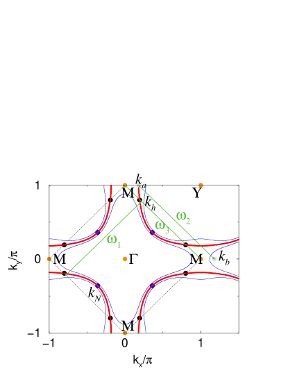
Figure 44: $(\pi,\pi)$-scattering geometry with definition of characteristic wavevectors and characteristic scattering energies discussed in the text. The thick curve is the Fermi surface. Lines of equal energy at $\pm 50$ meV around the Fermi energy are shown as thin curves.

The singular behavior of the susceptibility at certain energies $\omega$ can be studied analytically by expanding the normal state quasiparticle dispersion around the $(0,\pi)$ point and the $(\pi,0)$ point of the Brillouin zone up to quadratic order,

$$\xi(k_{x},\pi+k_{y}) = \xi_{M}+\alpha k_{x}^{2}-\beta k_{y}^{2}$$ (36)

$$\xi(\pi+k_{x},k_{y}) = \xi_{M}-\beta k_{x}^{2}+\alpha k_{y}^{2},$$ (37)

where the positive constants $\alpha$ and $\beta$ determine the effective masses of the dispersion around the $M$ point, and $\xi_{M}<0$ determines the position below the chemical potential of the saddle point singularity in the electronic dispersion.

In the normal state there is only one singularity, which is a (dynamic) Kohn singularity of square-root type. It corresponds to the wavevector which connects the Fermi surface point at ${\bf k}_{a}=(k_{a},\pi)$ (see Fig. 44) with the wavevector ${\bf k}_{b}={\bf k}_{a}+{\bf Q}=(\pi+k_{a},0)$ (or equivalent wavevectors). The corresponding energy is given by $\omega_{2}=|\xi_{b}|\approx|\xi_{M}|(1+\beta/\alpha)$, using that $k_{a}\approx\sqrt{-\xi_{M}/\alpha}$. The leading singular term of the susceptibility near $\omega_{2}$ can be readily calculated using the approximate dispersion Eqs. (36)-(37) [272, 273], and is of the form Const$-\frac{i}{\pi(\alpha+\beta)}\sqrt{\frac{1-\omega/\omega_{2}}{1-\beta/\alpha}}$. The behavior of the bare susceptibility is shown in Fig. 45 (a). In this figure the energy is measured in $J$, as this is the energy which determines the superconducting gap within the $t-t^{\prime}-J$ model used in these calculations [255, 256].

In the superconducting state, shown in Fig. 45 b-d, this singularity turns into a logarithmic singularity due to the qualitative change of the dispersion at the point ${\bf k}_{a}$. It shows a jump in the real part and a logarithmic divergence in the imaginary part of $\chi_{0}$, situated between the two absorption edges in Im$\chi_{0}$ (see figure). The corresponding energy is given by $\Delta_{a}+E_{b}$,

$$\omega_{2}=\Delta_{a}+\sqrt{\xi_{b}^{2}+\Delta_{b}^{2}}\;.$$ (38)

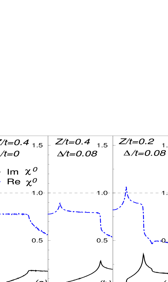
Figure 45: The irreducible susceptibility from Eq. (32) (in units of 1/4J) as function of energy at the antiferromagnetic wavevector. $Z$ is the distance of the saddle point singularity at the $(\pi,0)$ point in the fermionic Brillouin zone from the chemical potential, $Z=\mu-\epsilon_{M}=-\xi_{M}$. (a) is for the normal state, (b) for $Z\gg\Delta$, corresponding to underdoping, (c) corresponding to slight underdoping, and (d) for $Z\sim\Delta$ corresponding to optimal doping. The intersection of the dashed line with Re $\chi_{0}$ determines the resonance energy. (From Refs. [255, 256], Copyright ©2002 APS).

Above this singularity there is an absorption edge within the particle-hole continuum which corresponds to the wavevector which connects the $(\pi,0)$ point with the $(0,\pi)$ point. This singularity only exists in the superconducting state when there are states available at $(\pi,0)$ and $(0,\pi)$ above the chemical potential due to particle hole mixing. Calculations show, that the saddle point singularities near the $(\pi,0)$ and $(0,\pi)$ points ($M$ points) of the fermionic Brillouin zone play an important role. The distance of this saddle point singularity from the chemical potential, $Z=-\xi_{M}=-(\epsilon_{M}-\mu)$ introduces a parameter which quantifies its importance [254, 255]. The corresponding energy of the absorption edge is given in terms of this parameter by $2E_{M}$, or,

$$\omega_{3}=2\sqrt{\xi_{M}^{2}+\Delta^{2}}\;.$$ (39)

This absorption edge is seen in 45 (c) and (d). Note, that near optimal doping $\omega_{2}\approx\Delta+E_{M}$, and thus is close to $\omega_{3}=2E_{M}$. This can be seen in 45 (d).

Finally, in the superconducting state there is a continuum threshold toward low energies, which is given by twice the excitation energy at a momentum, which is slightly displaced from the ‘hot spots’ in direction toward the nodes of the order parameter. The hot spots are commonly defined as the crossing points between the Fermi surface and the lines $k_{x}\pm k_{y}=\pi$ ($k_{h}$ in Fig. 44). They are connected pairwise by antiferromagnetic wavevectors. In order to give an expression for the continuum threshold we consider the line $k_{x}+k_{y}=\pi$, and measure k along this line from $(0,\pi)$ toward $(\pi,0)$. It crosses the Fermi surface twice with angle $\alpha$ at the so called hot spot wavevectors. The order parameter at the first crossing point at $k_{h}$ will be denoted by $\Delta_{h}$ (the order parameter at the other hot spot along this line is then $-\Delta_{h}$), and we introduce velocities $v_{\Delta,h}=|\partial\Delta(k)/\partial k|_{k_{h}}$ and $v_{F,h}\sin\alpha=|\partial\xi(k)/\partial k|_{k_{h}}$. The continuum threshold is given by twice the excitation energy at a certain point along this line, which we determine by minimizing $2\sqrt{\xi(k)^{2}+\Delta(k)^{2}}$ with respect to $k$. Linearizing the $k$-dependence of $\xi_{k}$ and $\Delta_{k}$ around $k_{h}$ leads to

$$k-k_{h}=-\;\frac{\Delta_{h}v_{\Delta,h}}{v_{F,h}^{2}\sin^{2}\alpha+v_{\Delta,h}^{2}}\;.$$ (40)

The corresponding wavevector is displaced toward the nodal line $k_{x}=k_{y}$. From this the continuum threshold energy follows as

$$\omega_{1}=2\Delta_{h}\sqrt{1-\frac{2\beta_{h}^{2}}{\sin^{2}\alpha+\beta_{h}^{2}}},\quad\beta_{h}=\frac{v_{\Delta,h}}{v_{F,h}}\;.$$ (41)

Around optimal doing the correction term in the square-root is small and $k\approx k_{h}$, $\omega_{1}\approx 2\Delta_{h}$. The continuum threshold shows a jump in the imaginary part of the bare susceptibility, and a logarithmic singularity in the real part. It is seen in Fig. 45 (b)-(d) as the lowest-energy singularity.

The strength of this singularity at the continuum threshold $\omega_{1}$ depends on the position of the hot spots on the Fermi surface. When the hot spots move closer to the nodal points, which happens toward underdoping, the threshold energy decreases and the magnitude of the jump on the continuum threshold decreases, and vanishes completely at some critical doping. In the latter case the singularity is replaced by a square-root like singularity [250].

In the real part of the bare susceptibility the singularity shows up as a peak at the continuum edge, which leads to the development of a spin-excitonic mode below the continuum threshold, as we discuss next.

3.3 The resonance mode

3.3.1 Development of spin exciton

As can be seen from Eq. (30), for fixed momentum ${\bf q}$ the condition

$$1-J_{{\bf q}}\mbox{Re}\chi_{0}(\omega,{\bf q})=0,\;\;\mbox{Im}\chi_{0}(\omega,{\bf q})=0$$ (42)

gives sharp collective excitations at certain energies $\omega=\Omega_{res}$. This condition can be satisfied below the particle-hole continuum threshold $\Omega_{0}$, where it is of excitonic type. The weight of this collective excitation is given by

$$w_{\bf q}=\frac{1}{J_{\bf q}^{2}}\left(\frac{\partial\mbox{Re}\chi_{0}(\omega,{\bf q})}{\partial\omega}\Big{|}_{\omega=\Omega_{res}}\right)^{-1}.$$ (43)

As the real part of the bare susceptibility for a $d$-wave superconductor has a logarithmic singularity at the continuum threshold, the weight of the resonance goes linearly to zero when $\Omega_{res}$ approaches the continuum threshold $\Omega_{0}$. On the other hand, the weight diverges for $\Omega_{res}\to 0$.

At the antiferromagnetic wavevector, ${\bf q}={\bf Q}$, the corresponding exciton is the resonance mode observed in INS experiments. The susceptibility can then be written as the sum of a continuum part and a resonant part, and the latter is given through its imaginary part

$$\mbox{Im}\chi_{res}(\omega,{\bf Q})=\pi w_{\bf Q}\left(\delta(\omega-\Omega_{res})-\delta(\omega+\Omega_{res})\right)\;.$$ (44)

Collective excitations stay well defined also for $\mbox{Im}\chi_{0}(\omega,{\bf q})\neq 0$ as long as

$$|J_{{\bf q}}\mbox{Im}\chi_{0}(\Omega_{res},{\bf q})| \ll 1$$

$$|J_{{\bf q}}^{2}w_{\bf q}\mbox{Im}\chi_{0}(\Omega_{res},{\bf q})| \ll \Omega_{res}$$ (45)

holds. As we do not consider a spin-density wave instability, the condition

$$1-J_{{\bf q}}\mbox{Re}\chi_{0}(0,{\bf q})>0$$ (46)

is necessary. In the following we discuss the resulting resonance feature as a function of various parameters.

3.3.2 Doping dependence

Calculations within a $t-t^{\prime}-J$ model in mean-field approximation lead to doping and temperature dependent effective hopping parameters $\tilde{t}$, $\tilde{t}^{\prime}$ and $\tilde{t}_{\perp}$. Calculations using a slave-boson technique were performed by Brinckmann and Lee [225, 250], calculations in a Hubbard operator technique by Onufrieva and Pfeuty [255, 256]. The Mori memory-function formalism has been applied by Sega, Prelovšek and Bonča [257, 258, 259].

Figure 46: Magnetic response at wave vector $(\pi,\pi)$ for a single CuO₂ layer for optimal to underdoped (left) and for optimal to overdoped (right) hole filling $x$. Optimal doping corresponds to $x=0.12$. The calculations are for $T=0$. The hole fillings for the right picture are $x=0.12(a),0.14(b),0.18(c),0.24(d),0.30(e)$. The main figures show Im $\chi_{0}$ calculated from Eq. (32). The insets show the corresponding Im $\chi$ calculated from Eq. (30), and using a damping term $\Gamma=$2.5 meV in Eq. (32). (From Ref. [250], Copyright ©2001 APS).

In Fig. 46 the doping dependence of both Im$\chi_{0}$ and Im$\chi$ (in the insets), obtained with a slave-boson technique, is shown. With underdoping the continuum threshold $\omega_{1}$ moves to lower energies, and at the same time the magnitude of the jump decreases. At a critical doping value the jump vanishes and the continuum threshold shows a weak square-root singularity. The resonant mode, shown in the inset, moves to lower energies and its weight increases. With overdoping the continuum threshold first increases, then decreases again. A similar trend shows up for the resonance frequency [250]. The qualitative behavior of the experimentally observed doping dependence thus is reproduced by these $t-t^{\prime}-J$ model calculations.

In Ref. [29] the doping dependence of the resonance mode was studied in a self-consistent FLEX approximation combined with random phase approximation. It was found that in the overdoped range the resonance is close to twice the maximal superconducting $d$-wave gap $2\Delta$, at optimal doping is given by $\Omega_{res}=2\Delta_{0}-\Omega_{max}$ (with the normal state spin-fluctuation spectrum given by Im$\chi(Q,\Omega)=$Im$[\chi_{Q}/(1-i\Omega/\Omega_{max})]$) and in the underdoped regime follows the normal state spin-fluctuation frequency $\Omega_{max}$.

In Ref. [17] the two limiting cases of weak and strong spin-fermion coupling were studied in an effective low-energy theory. There it was found that for the weak coupling limit, where $\Delta\ll\Omega_{max}$ (corresponding to strongly overdoped materials), the resonance position $\Omega_{res}=2\Delta_{h}(1-w_{\bf Q})$ is related to the weight of the resonance, $w_{{\bf Q}}=e^{-\Omega_{max}/(2\Delta_{h})}$ (here, $\Delta_{h}$ is the gap at the ‘hot-spot’ wavevector ${\bf k}_{h}$, see Fig. 44). Thus, the binding energy of the resonance, $2\Delta_{h}-\Omega_{res}$, is proportional to the weight of the resonance $w_{{\bf Q}}$. In the strong coupling limit, appropriate for the underdoped region, they obtain $\Omega_{res}\sim\sqrt{\Omega_{max}\Delta_{h}}$. This is valid when $\Omega_{res}<\Delta$, $\Omega_{max}<\Delta$ holds. Both inequalities are fulfilled for optimally and underdoped materials.

3.3.3 Dependence on disorder

There have been few theoretical efforts to study the influence of non-magnetic impurities on the magnetic resonance. In Ref. [275] the effects of dilute Zn impurities on the spin susceptibility in YBa₂Cu₃O_7-δ was studied using a two-dimensional Hubbard model. Coulomb correlations were included via the random-phase approximation, before averaging over the positions of the impurities was performed. An enhancement of the static susceptibility at the antiferromagnetic wavevector with Zn impurity concentration was found.

A different route was chosen in Ref. [276], by studying a quantum impurity in a system of coupled spin-ladders, which exhibits a paramagnetic ground state for small inter-ladder coupling. It was argued there that the magnon damping mechanism due to the presence of impurities in such systems has also relevance for the broadening of the resonance peak in Zn-doped YBa₂Cu₃O₇.

Further theoretical work in studying the interplay between non-magnetic impurities and antiferromagnetic correlations in superconducting cuprates is required for a complete understanding of the experimental results of Section 2.1.6.

3.3.4 Dependence on magnetic field

In order to explain the suppression of the weight of the magnetic resonance with an applied magnetic field in $c$-axis direction [122], it is necessary to consider the influence vortices have on it. This problem was treated in Ref. [277]. There are several possible effects of vortices. The first effect is associated with the influence of the supercurrents circulating around the vortices on the resonance. Second, there might be an effect of a spatially uniform suppression of the $\langle\Delta_{{\bf k}}\Delta_{{\bf k}+{\bf Q}}\rangle$ correlator which enters the coherence factors of the spin susceptibility (where ${\bf Q}$ is the antiferromagnetic wave vector at which the resonance is peaked). Such a suppression could be a result of dephasing of the pairing in a c-axis field due to the vortices, as observed in Josephson plasma resonance experiments [278]. It can be taken into account by reducing $\alpha$ to less than 1 in Eq. (32). A related model was considered to explain a sum rule violation in c-axis infrared conductivity, see [274]. A third possibility is an assumed (field induced) spatially uniform suppression of the gap magnitude. Finally, the effect of the vortex cores will have an impact. In this case the resonance might be locally suppressed in the core regions and recovers only outside. This assumes of course that the spin correlation length is short, so that a local suppression of the resonance feature makes sense. Indeed, in cuprates the correlation length associated with the resonance is of the same order as the superconducting coherence length. The fact that the experimental suppression goes like $1-H/H^{*}$ (where $H^{*}$ is a number of the order of the upper critical field) is highly suggestive of a vortex core effect [122].

A calculation of the influence of the supercurrents around the vortices on the resonance in the spin-spin correlation function has shown that the supercurrent has three effects: it shifts the position of the resonance to slightly lower energy, it broadens the resonance, and it reduces the magnitude of the resonance at the peak energy [277]. However, the integrated weight between 0 and $\approx 2\Delta$ is conserved. These findings are in apparent contradiction with the experimental facts, which are that the resonance does not shift, nor broaden, and that the integrated weight is reduced by about 15% at 7 T ( [122]).

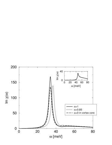
Figure 47: Left: Comparison of zero field susceptibility with the same susceptibility, but with reduced gap magnitude, $\Delta$. Dotted line: assuming a spatially uniform reduction from 29 meV to 20 meV; dashed line: assuming a reduction to zero in 24% of the vortex unit cell area representing the cores (the uniform zero gap response is shown in the inset). In both cases the weight of the resonance is reduced, but for the spatially uniform case, the resonance is shifted considerably downwards in energy. Right: Comparison of zero field susceptibility with the same susceptibility, but with the $\langle\Delta\Delta\rangle$ correlator in the numerator of Eq. (32) reduced ($\alpha<1$). Dotted line: assuming a spatially uniform reduction by 15%; dashed line: assuming a reduction to zero in 20% of the vortex unit cell area representing the cores (the uniform zero $\alpha$ response is shown in the inset). In both cases the weight of the resonance is reduced, but for the spatially uniform case, the resonance is shifted considerably upwards in energy. (From Ref. [277], Copyright ©2001 APS).

In Fig. 47 the results for the influence of a magnetic field on the resonance are summarized. First, any spatially homogeneous effect is in disagreement with the experimental data: (A) a homogeneous reduction of the gap magnitude, shown as the dotted line in in the left panel of Fig. 47, leads to a shift of the resonance to considerably lower energy compared to the zero field result (full line); and (B) a homogeneous reduction of the $\langle\Delta\Delta\rangle$ correlator by 15% ($\alpha=0.85$), shown as dotted line in the right panel of Fig. 47, leads to a shift of the resonance to higher energy, compared to the zero field result (full line).

The vortex-core effect is illustrated as dashed lines in Fig. 47. In the insets the susceptibilities for zero $\Delta$ and for zero $\langle\Delta\Delta\rangle$ correlator, used in the vortex core area, are shown, whereas the full curves of the main panels are used for the inter-vortex regions. The latter is justified since the Doppler shift has a negligible effect on the integrated intensity. In both cases, the resulting curves, calculated for a 15% reduction in total integrated weight, reproduce very well the experimental finding of no shift or broadening of the resonance.

The conclusion that the resonance is not supported in the region of the vortex core is corroborated by the following five additional facts [277]: a) the considerable momentum width of the resonance shows that the corresponding spin excitations have a decay length of only two lattice constants, which is smaller than the coherence length; thus the resonance will be sensitive to variations of the order parameter on the coherence length scale; b) the resonance at zero field only exists in the superconducting state, and disappears in the normal state; c) coherence peaks in the single particle density of states at the gap edge were not found in the core region in STM measurements [279, 280, 281]; this would modify the $2\Delta$-edge in $\chi^{\prime\prime}_{0}$ [Eq. (32)] and suppress the resonance; d) in underdoped materials, missing subgap states point toward a loss of quasiparticle weight due to a pseudogap in the vortex core [279, 280, 281]; e) the dip feature in the tunneling density of states, thought to be due to the coupling of quasiparticles to the resonance [7], is not observed in the vortex core region [279, 280, 281].

As documented by ARPES measurements [282, 283], quasiparticle-like peaks in the spectral functions are present only below $T_{c}$, the onset temperature of phase coherence. Motivated by this observation it was suggested in Ref. [277] that this may lead to a destruction of quasiparticle excitations in the vortex core region similar to what happens in the pseudogap state. The absence of quasiparticle peaks as well as of the neutron resonance in the core region is consistent with the notion that both these spectral features require substantial local phase correlations [121]. Thus, we can assume that the magnetic resonance is simply absent in the vortex core regions because of the absence of quasiparticle excitations [277]. The question to whether the vortex core is closely related to the pseudogap phase, or if even a different type of order exists in the core region, is not settled up to now and subject of ongoing research.

3.3.5 Even and odd mode in bilayer cuprates

For bilayer materials the susceptibility is classified into even and odd components according to Eqs. (4)-(5) and (7)-(8). It can be inferred experimentally via Eqs. (3) and (6).

If the coupling between the two planes in the bilayer is coherent, then the bands split into bonding and antibonding bands according to Eq. (12). The $d$-wave order parameter has the form Eq. (15). In agreement with experiments [174] it is assumed to be the same on the bonding and antibonding bands.

The irreducible susceptibility, Eq. (32), is generalized to a matrix in bonding and antibonding indices, and for example the component $\chi_{0}^{(ab)}$ reads,

$$\chi_{0}^{(ab)}(\omega,{\bf q}) = -\sum_{{\bf k}}\sum_{\mu,\nu=\{\pm\}}\frac{A^{(a),\mu}_{{\bf k}}A^{(b),\nu}_{{\bf k}+{\bf q}}+\alpha^{(ab)}_{\bf q}C^{(a),\mu}_{{\bf k}}C^{(b),\nu}_{{\bf k}+{\bf q}}}{\omega+E^{(a),\mu}_{{\bf k}}-E^{(b),\nu}_{{\bf k}+{\bf q}}+i\Gamma^{(ab)}}$$ (47)

$$\times\left(f(E^{(a),\mu}_{{\bf k}})-f(E^{(b),\nu}_{{\bf k}+{\bf q}})\right)\;.$$

with coherence factors and excitation energies calculated with the corresponding bonding and antibonding dispersions and order parameters. One then builds even and odd components of the irreducible susceptibility according to Eq. (7). Taking into account an exchange coupling between the planes within a bilayer, the exchange coupling also has even and odd components

$$J^{e}_{\bf q}=J_{\bf q}-J_{\perp},$$

$$J^{o}_{\bf q}=J_{\bf q}+J_{\perp}.$$ (48)

The susceptibility then can be written as

$$\chi_{e}(\omega,{\bf q})=\frac{\chi^{(e)}_{0}(\omega,{\bf q},p_{z})}{1-J^{(e)}_{{\bf q}}\chi^{(e)}_{0}(\omega,{\bf q})}\;,$$

$$\chi_{o}(\omega,{\bf q})=\frac{\chi^{(o)}_{0}(\omega,{\bf q},p_{z})}{1-J^{(o)}_{{\bf q}}\chi^{(o)}_{0}(\omega,{\bf q})}\;.$$ (49)

Results of calculations for the spin susceptibility taking into account bilayer splitting are reproduced in Fig. 48 for two doping levels.

Figure 48: Imaginary part of odd- and even-mode susceptibility of a bilayer system at wavevector $(\pi,\pi)$. (From Ref. [250], Copyright ©2001 APS).

The even-mode susceptibility shows a considerably weaker resonance feature, which is placed closer to the continuum edge, than the odd-mode susceptibility. This is consistent with the experimental observation of [116].

3.4 The incommensurate response

There are numerous theoretical works explaining the incommensurate response in the spin susceptibility [228, 229, 255, 17, 225, 284, 251, 29, 256, 264, 268, 134].

In a picture where the magnetic resonance mode is treated as an excitonic bound state below the particle-hole continuum, the incommensurate response arises from the resonance condition for wavevectors slightly displaced from the antiferromagnetic wavevector. For this case, the continuum threshold for a $d$-wave superconductor shows a characteristic dependence on $\delta_{x}=q_{x}-\pi$, with a minimum in the continuum threshold $\omega_{1}(\delta_{x})$ at a certain value $\pm\delta_{x,min}$. As a consequence, the resonance criterion is fulfilled also for wavevectors with non-zero $\delta_{x}$. For $\delta_{x}\neq 0$ the step in Im $\chi_{0}$ splits into two steps, the lower of which corresponds now the the continuum threshold. The stepsize is however much smaller than the total stepsize at $\delta_{x}=0$, leading also the a weaker structure in Re $\chi_{0}$. Thus, the weight of the resonance feature drops quickly for increasing $|\delta_{x}|$. This behavior is shown in Fig. 49 (left), where a tight-binding dispersion obtained from ARPES data for Bi₂Sr₂CaCu₂O_8+δ was used as input [268]. Interestingly, for this case the dispersion of the collective mode is rather weak near the resonance energy $\Omega_{res}$, which leads to a large momentum width of the resonance mode as observed in experiments. Also shown in Fig. 49, on the right, is an example for the theoretical results appropriate for an underdoped YBa₂Cu₃O_6.85 sample [134], reproducing details of the incommensurate dispersion which are shown in Fig. 8. In particular, it explains a new feature, the so-called $Q^{\ast}$ mode (light arrow), which resides above the resonance mode (dark arrow) at incommensurate wavevectors and was observed in the experiment [92].

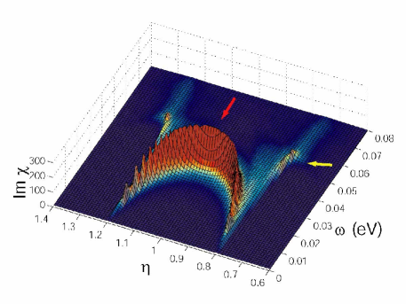
Figure 49: Left: Dispersion along the (110) direction and intensity of the spin-1 resonance from Eqs. (30)-(32) using a tight-binding quasiparticle dispersion inferred from ARPES experiments, corresponding to optimally doped Bi₂Sr₂CaCu₂O_8+δ. The parameter $J_{{\bf q}}\equiv J_{0}$ was chosen to be independent of the wavevector ${\bf q}$. (From Ref. [268], Copyright ©2001 APS). Right: The same for parameters suitable to reproduce the experimental dispersion along the (110) direction of an underdoped YBa₂Cu₃O_6.85 sample, as shown in Fig. 8. Here, $\Delta=42$ meV, and $J_{{\bf q}}=573$meV$[1-0.1(\cos q_{x}-\cos q_{y})]$ was used, to reproduce details in the experimental dispersion of experiment [92] (indicated by arrows). (From Ref. [134], Copyright ©2005 APS).

The incommensurability pattern below the resonance is characteristic in the sense that it has four maxima at positions $(\pi\pm\delta_{x},\pi)$, and $(\pi,\pi\pm\delta_{x})$. This is reproduced quantitatively by theory using the formulas Eqs. (30)-(32) [225, 284, 251, 256, 258, 134]. An example is shown in Fig. 50.

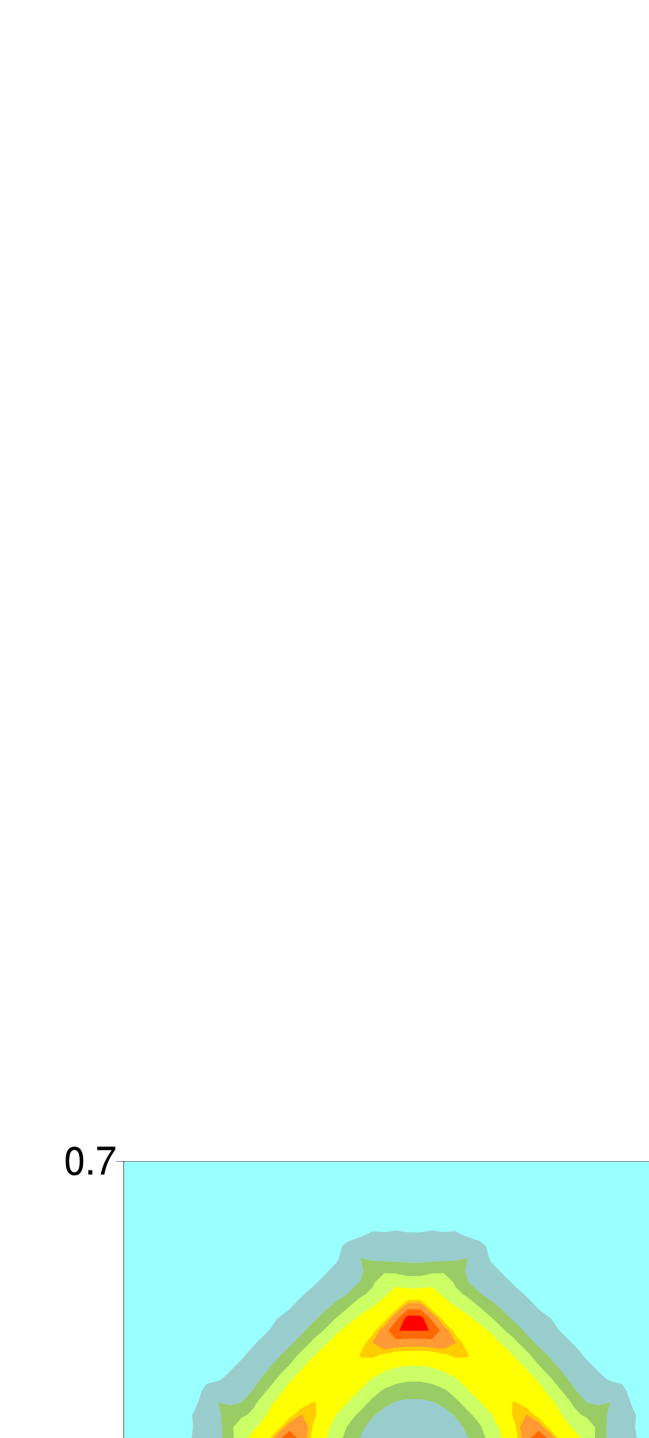
Figure 50: $p_{x}$, $p_{y}$ dependence of Im $\chi({\bf p},\omega)$ showing the incommensurate response around the $(\pi,\pi)$ wavevector (corresponding to $p_{x}=p_{y}=0.5$). Left the theoretical calculation [255, 256] according to Eqs. (30), (32), for a $t-t^{\prime}-J$ model with $t^{\prime}/t=-0.3,Z/t=0.2,\Delta/J=0.2,\Omega/J=0.23$. Right, experimental results from [88], measured on YBa₂Cu₃O_6.6 at $\omega=24$meV. (From Ref. [255, 256], Copyright ©2002 APS).

Corresponding experimental patterns above the resonance have their maxima at positions $(\pi\pm\delta^{\ast},\pi\pm\delta^{\ast})$ [115], consistent with theory [134, 258, 259].

3.5 Effective low-energy theories

A different approach is to start from a separation of energy scales into high energy and low energy. On a formal level this allows for a perturbation expansion in Feynman diagrams, where all propagators are written as a sum of a high-energy propagator and a low-energy propagator. Then, all high-energy propagators are combined with their attached interaction vertices to new, renormalized high-energy interactions. The resulting diagrams contain low-energy propagators and high-energy effective interaction vertices. In a second renormalization step the quasiparticle renormalization factor $z_{0}$ is absorbed by the attached vertices to built quasiparticle propagators and effective quasiparticle interaction vertices. For theoretical treatments along these lines see e.g. Abanov et al. [285] and citations there.

Using this procedure for the susceptibility $\chi$, one usually neglects terms containing one low-energy propagator and one high-energy propagator in $\chi_{0}$, so that one has a high-energy bare susceptibility $\chi_{h}$ and a low-energy bare susceptibility $\chi_{l}$. For the full susceptibility one obtains (we omit for simplicity all arguments and we allow for a more general notation, where multiplication of two quantities can for example also symbolize convolutions)

$$g_{1}\chi g_{2} = g_{1}\frac{(\chi_{h}+z_{0}\chi_{l}z_{0})}{1-J(\chi_{h}+z_{0}\chi_{l}z_{0})}g_{2}$$ (50)

$$= (g_{1}\chi g_{2})_{\rm inc}+\bar{g}_{1}\frac{\chi_{l}}{1-\bar{J}\chi_{l}}\bar{g}_{2}$$ (51)

with the renormalized quantities

$$(g_{1}\chi g_{2})_{\rm inc} = g_{1}\chi_{h}\frac{1}{1-J\chi_{h}}g_{2}$$ (52)

$$\bar{g}_{1} = g_{1}\frac{1}{1-\chi_{h}J}z_{0}$$ (53)

$$\bar{g}_{2} = z_{0}\frac{1}{1-J\chi_{h}}g_{2}$$ (54)

$$\bar{J} = z_{0}\frac{1}{1-J\chi_{h}}Jz_{0}\;.$$ (55)

The renormalization factors $z_{0}$ entering $\chi_{l}$ are in general anisotropic, and are defined as $\sqrt{z_{{\bf k}}z_{{\bf k}+{\bf q}}}$. Thus, the vertices for the effective low-energy susceptibility depend in general both on the quasiparticle wavevector ${\bf k}$ and the external wavevector ${\bf q}$.

We assume that these renormalized high-energy quantities vary on a high-energy scale, and can be considered in first approximation as constant in energy when considering the low energy region. If one chooses to assign some energy-dependence to these quantities, then it is very weak in the low-energy region. Only $\chi_{l}$ is affected by the superconducting transition, $(g_{1}\chi g_{2})_{\rm inc}$, $\bar{J}$ and $\bar{g}_{1,2}$ stay unaffected. If one wants to allow for a change of the quasiparticle renormalization factors at $T_{c}$ one needs to keep them explicitly. However, up to date it is not clear yet, if for high-$T_{c}$ cuprates the loss of the coherence peaks is due to a change in $z_{0}$ or due to a dramatic decrease of the lifetime [189]. Note in this regard, that the experimental definition of the coherent quasiparticle weight in ARPES is purely phenomenological and might be different from the above introduced quasiparticle renormalization factors.

We are interested in strong correlations which lead to

$$\frac{1}{1-J\chi_{h}}\gg 1\;$$ (56)

at the antiferromagnetic wavevector. This means, all ‘external’ effective coupling constants (e.g. $\bar{g}_{1}$,$\bar{g}_{2}$) as well as the effective exchange coupling $\bar{J}$ are strongly enhanced at the antiferromagnetic wavevector. The same is true for the incoherent part $(g_{1}\chi g_{2})_{\rm inc}$, which determines the real part of the susceptibility at the antiferromagnetic wavevector at $\omega=0$. For the calculation of $\chi_{l}$ the high-energy part of the quasiparticle dispersion is not essential, as any re-definition of the separation procedure in high- and low-energy quantities goes along with a corresponding change in the interaction constants exactly in a way that physical measurable quantities are not affected. Note that low-energy quantities are insensitive to the details of this renormalization procedure.

As an example, when using tight-binding dispersion fits, the high-energy part of the dispersion can be chosen arbitrarily without changing the low-energy physics. One has to bear in mind, however, that the interaction constants for the quasiparticles do depend on the choice of the high-energy dispersion (bandwidth, high-energy cut-off etc.) as this determines their ‘coherent quasiparticle weight’. Thus, only if it is specified if the high-energy quasiparticle renormalization factor is included in both the coupling constants and high-energy dispersions or not, it makes sense to compare coupling constants in different theories.

With this in mind, the formulas (30) and (32) can be used with a dispersion obtained from tight-binding fits to experimental data near the Fermi energy, and choosing any reasonable behavior for high energies, assuming that all coupling and interaction constants are renormalized quantities assigned to the particular choice of the high-energy part of the dispersion.

If one is interested in the behavior near the antiferromagnetic wavevector only, a common procedure is to expand the quantity $1-J\chi_{h}$ according to

$$1-J_{\bf q}\chi_{h}(\omega,{\bf q})\approx\kappa^{2}+\xi_{0}^{2}({\bf q}-{\bf Q})^{2}-\frac{\xi_{0}^{2}\omega^{2}}{v^{2}_{s}}\;,$$ (57)

where $v_{s}$ is a spin-wave velocity, $\xi_{0}$ is an antiferromagnetic correlation length, and $\kappa^{-2}$ determines the enhancement of the normal state static susceptibility at the antiferromagnetic wavevector. The $\omega$ dependence is relevant only for the case that $\kappa$ becomes small. This introduces a new low-energy scale, and the separation between high energies and low energies is not anymore clear cut. This case corresponds to strongly underdoped cuprate superconductors, where the pseudogap phenomenon is dominating the physics. For overdoped, optimally doped and slightly underdoped materials the spin-wave term can be neglected.

The condition for a resonance in the superconducting state follows now from Eq. (51) as

$$J_{\bf Q}\mbox{Re}\chi_{l}(\omega,{\bf Q})=\kappa^{2}$$ (58)

which replaces the condition $J_{\bf Q}\mbox{Re}\chi_{0}(\omega,{\bf Q})=1$.

A general low-energy theory for small deviations from the antiferromagnetic wavevector and small energies would start from Eq. (50), using Eq. (57) in the denominator, and neglecting $\chi_{l}$ in comparison with $\chi_{h}$ in the numerator (in the denominator $\chi_{l}$ cannot be neglected against $\chi_{h}$ because $1-J\chi_{h}$ is comparable to $Jz_{0}^{2}\chi_{l}$ even though $Jz_{0}^{2}\chi_{l}\ll J\chi_{h}$). The high-energy quantities $\chi_{h}$ and $\xi_{0}^{2}$ are renormalized by $\kappa^{-2}$ according to $\xi=\xi_{0}/\kappa$, $\chi_{Q}=\chi_{h}/\kappa^{2}$. It is common to introduce a self energy $\Pi$ via $Jz_{0}^{2}\chi_{l}/\kappa^{2}=\bar{g}^{2}\chi_{Q}\Pi$, which enters the Ornstein-Zernicke form for the susceptibility in the following way,

$$\chi(\omega,{\bf q})\approx\frac{\chi_{Q}}{1+\xi^{2}({\bf q}-{\bf Q})^{2}-\bar{g}^{2}\chi_{Q}\Pi({\bf q},\omega)}\;.$$ (59)

The imaginary part of $\chi(\omega,{\bf q})$ is not a high-energy quantity, but enters even in the normal state only via the low-energy quantity $\Pi({\bf q},\omega)$.

The use of the above procedures is a powerful way to discuss dispersion features in the spin-spin response function [267, 17, 268, 134] and to describe the low-energy physics near the Fermi surface. It is however semi-phenomenological in the sense that (in general momentum dependent) interaction parameters and high-energy contributions to the real part of the spin-susceptibility have to be obtained from either experiment or more general theories.

3.6 Magnetic coherence in La_2-xSr_xCuO₄

Since the material La_2-xSr_xCuO₄ shows a spin excitation spectrum different from the one discussed in the previous sections, we briefly summarize here the modifications of the theory that are necessary to describe the spin-response of this system.

The spectrum of the single layered compound La_2-xSr_xCuO₄ has been scrutinized experimentally both in the normal and superconducting state. The following important modifications in comparison with the cuprates having optimal temperatures around 90 K exist: (A) In the normal state the spectrum for $x>0.04$ is characterized by peaks at incommensurate planar wavevectors ${\bf Q}_{\delta}=(\pi(1\pm\delta)),\pi)$ and $(\pi,\pi(1\pm\delta))$ [111, 112, 90, 113], where $\delta$ increases with increasing doping. (B) When entering the superconducting state $\chi^{\prime\prime}(\omega,{\bf Q}_{\delta})$ is reduced from its normal state value for $\omega<7$ meV, and increases for $\omega{{}_{\textstyle>}\atop{\textstyle\sim}}7$ meV; $\chi^{\prime}(\omega,{\bf Q}_{\delta})$ decreases in the superconducting state [135]. (C) For $\omega\approx 7$ meV the incommensurate peaks sharpen in the superconducting state [112, 135].

These effects, termed “magnetic coherence effects” [112], have been explained theoretically [270, 271], based on a modified form of Eq. (59). The main difference between the behavior in the spin susceptibility for La_2-xSr_xCuO₄ and that for the systems YBa₂Cu₃O_6+x, Bi₂Sr₂CaCu₂O_8+δ, and Tl₂Ba₂CuO_6+δ is, that for La_2-xSr_xCuO₄ the momentum dependence of the high-energy contributions to the spin susceptibility in the vicinity of the antiferromagnetic wavevector cannot be neglected. Thus, the detailled momentum dependence on the left hand side of Eq. (57) is important, and its presence leads to the incommensurate spin response in the normal state. This can be described by an expansion similar to Eq. (57), however around the incommensurate wavevectors ${\bf Q}_{\delta}$. The third term in the modified Eq. (57), though, can be neglected for not too strongly underdoped compounds, as experimentally one finds that the normal state low-energy spin excitation spectrum is almost dispersionless in these cases.

In the normal state the real part of $\Pi$ in the denominator of Eq. (59) is proportional to the particle-hole asymmetry of the fermionic dispersion around the chemical potential, which is small near the Fermi surface points connected by the incommensurate magnetic wavevectors. Thus, the position of the incommensurate peaks is determined to a good approximation by high-energy fermions only. In contrast, the momentum width of these incommensurate peaks is determined by damping due to coupling to low-energy quasiparticles, as it comes from the bosonic self-energy $\Pi$ in the denominator of Eq. (59).

In the superconducting state the quantity $\Pi({\bf q},\omega)$ changes in two ways: it develops a non-negligible real part, and its imaginary part is strongly modified at low $\omega$ due to the presence of the anisotropic superconducting gap. The latter fact causes restrictions in the damping of spin-excitations, that lead to a sharpening of the incommensurate peaks.

The calculations of Refs. [270, 271] along these lines give a good account of the experimental facts, and in particular reproduces (A) the frequency dependence of $\chi^{\prime\prime}$ at the incommensurate wavevectors in the normal and superconducting states, (B) the momentum dependence of the spin gap in the superconducting state, (C) the changes of the momentum width of the incommensurate peaks when entering the superconducting state, and (D) the slight dispersion towards the antiferromagnetic wavevector with increasing frequency in the superconducting state [270]. It was argued by the same authors that the low-energy incommensurate dispersion in YBa₂Cu₃O_6+x can be explained in a similar way.

Finally, it is important to note that the magnetic resonance mode as described in previous sections arises from the dependence of $\Pi({\bf q},\omega)$ on frequency $\omega$ in Eq. (59). From Eq. (57) it follows that by adding the spin-wave term (third term on the right hand side) to the high-energy contribution of the spin susceptibility, one can expect a similar resonance effect. This was theoretically studied in Ref. [267]. Note that these two descriptions are conceptually very different, as in one case high-energy fermions are responsible for the formation of the resonance mode, whereas in the other case it is the low-energy quasiparticles that are responsible. For optimally and overdoped materials one would, however, expect that one can safely neglect any spin-wave term in the normal state response. For the underdoped region the presence or absence of such a term is far from being settled (note that the strong damping by low-energy quasiparticles in the normal state makes the experimental observation of such a term non-trivial).

4 Coupling of quasiparticles to the magnetic resonance mode

The key question for any understanding of the importance of magnetic excitations for high-$T_{c}$ superconductivity is how strongly do quasiparticles couple to spin fluctuations. The observation of clear correlations between the magnetic spin-1 mode and the self-energy effects in the single-particle spectrum opens the possibility to determine experimentally the strength of this coupling. This is extremely valuable for theoretical treatments, which up to now do not even agree on the order of magnitude of the coupling constant[286, 23]. In order to achieve this goal, several experimental difficulties had to be overcome, and it is only very recently that the precision of ARPES experiments became sufficient to allow for the separation of the effects of the magnetic resonance from other effects like bilayer splitting and features due to electron-phonon coupling [49]. With regard to the latter point, a sharp, weakly dispersing phonon mode, if dominating in the phonon spectrum, would in a similar way allow for the determination of the coupling constants between electronic quasiparticles and phonons. However here we concentrate on the more controverse coupling between electronic quasiparticles and magnetic excitations.

An assignment of the anomalous ARPES lineshape near the $M$ point of the Brillouin zone to the coupling between spin fluctuations and electrons has been made in a number of theoretical treatments [8, 10, 11, 28, 14, 15, 16, 17, 7]. In particular, the idea that a dispersionless collective mode is coupled strongly to electronic quasiparticles was suggested by Norman et al. [15, 16] and by Shen and Schrieffer [14]. By analogy with the Holstein effect, the coupling of the magnetic resonance to electronic quasiparticles should lead to spectral anomalies (“dips”) in the fermionic spectral function, most prominent near the $(\pi,0)$ points of the fermionic Brillouin zone [4], because these are connected by the characteristic wavevector of the resonance. The separation between the quasiparticle peak and the dip should equal the resonance energy [16, 17]. The EDC dispersion shows a break at roughly the same energy and the MDC dispersion an $S$-shape anomaly. The universality of this energy scale can be explained in a unified picture [7, 24, 25]. At the same time, for not too strongly overdoped materials this coupling leads to a kink in the quasiparticle dispersion along the $(\pi,\pi)$ direction [33, 34, 38], with the kink energy near $\Delta+\Omega_{res}$ [7]. A kink-like feature is also present above $T_{c}$ in underdoped and optimally doped materials, due to a peak in the spin-fluctuation spectrum. However, it sharpens when entering the superconducting state. For overdoped materials, the effect at the nodes due to the spin resonance becomes weak and is overshadowed by additional effects, most probably phonons, which add to the modification of the nodal dispersion. Similarly, effects of the magnetic resonance are expected for the density of states, as measured by tunneling spectroscopy, and were found both in the SIN and SIS tunneling conductance [44]. Finally, also in optical conductivity [287, 220, 45] such self-energy effects are present at $2\Delta+\Omega_{res}$ [17, 21, 221, 288] and at $\Delta+\Omega_{\rm res}$ [220, 221]. The magnetic resonance mode can also cause subgap peaks in SNS junctions [289].

Experimentally, as it was discussed in section 2, the features that could be interpreted as due to scattering from the resonance have been observed in ARPES spectra, SIN and SIS tunneling spectra, and optical conductivity measurements on Bi₂Sr₂CaCu₂O_8-δ at various doping concentrations [22]. Furthermore, the resonance energies inferred from ARPES [32] and SIS [44] measurements as a function of doping match $\Omega_{res}$ as measured directly by inelastic neutron scattering. The mode extracted from SIS experiments [44] is located very near $2\Delta$ in overdoped materials, but progressively deviates to lower energies with underdoping, as would be expected of a collective excitation inside a continuum gap [44]. In addition, the real part of the fermionic self-energy at the node as a function of temperature has been shown to scale with the resonance intensity [38]. In recent years, such self-energy effects have been also separated from bilayer splitting effects and have been shown to be present independently [163, 178].

The minimal set of characteristic features for the collective mode which is involved follows from the experimental results from ARPES and tunneling. The mode is characterized by its energy and its intensity at the $(\pi,\pi)$ wavevector (the wavevector being suggested by the momentum dependence of the strength of the ARPES anomalies). Its properties from ARPES and SIS tunneling are as follows. The energy should be weakly dependent on momentum, roughly 40 meV in optimally doped cuprates, follow $T_{c}$ with doping, and be constant with increasing temperature up to $T_{c}$. The intensity should be maximal at the $(\pi,\pi)$ wavevector, where it should increase with underdoping and follow an order parameter-like behavior as a function of temperature below $T_{c}$. The mode should be absent in the normal state; a remnant can be present in the pseudogap state, but an abrupt increase in intensity should occur at $T_{c}$ with lowering temperature. It is clear that these characteristics extracted from ARPES and tunneling spectra fit perfectly to the magnetic-resonance mode.

The first question in order is, if the coupling between the magnetic resonance mode and the electrons is sufficient to lead to the correct order of magnitude of the self energy effects in the electronic dispersions as observed in experiment.

4.1 The coupling constant and the weight of the spin resonance

The issue we will discuss in this section is whether the magnetic resonance can account for the measured changes in the fermionic properties of the cuprates below $T_{c}$, via a feedback effect similar to the Holstein effect in phonon mediated superconductors. It was pointed out by Kee et al. [286] that this is not obvious, since the total experimental spectral weight of the resonance peak,

$$I_{0}=\int S({\bf q},\Omega)\frac{d^{2}qd\Omega}{8\pi^{3}},$$ (60)

is only a few percent of the local moment sum rule, $S(S+1)/3=1/4$. Here, we set $\mu_{B}=1$ and for $S=1/2$ define the spin structure factor as

$$S({\bf q},\Omega) = \int dt\int d^{2}re^{i(\Omega t-{\bf q}{\bf r})}<S_{x}({\bf r},t)S_{x}({\bf 0},0)>$$ (61)

$$= \frac{0.5\hbar}{1-e^{-\hbar\Omega/k_{B}T}}\chi^{\prime\prime}({\bf q},\Omega).$$

This local moment sum rule is, however, only valid in in the Heisenberg limit, and the total integrated weight of the structure factor should be reduced in the metallic regime.

Motivated by the raised doubts of Ref. [286], Abanov et al. [23] addressed the issue whether the smallness of the integrated intensity of the peak precludes strong effects on the fermions. Their main result is that the fermionic self-energy due to scattering from the resonance is strong and unrelated to the small integrated intensity of the peak.

The question can be divided into two key points: first, what the order of magnitude for the values of the spin-fermion coupling $g$ and the dimensionless coupling constant $\lambda$ is, and second, the dependence of the self-energy on the integrated intensity of the peak.

The second question was dealt with already in Refs. [17, 7, 23, 24, 25], where detailed numerical calculations have shown that under the assumption that the coupling constant is of the order of several hundred meV, the small but finite weight is enough to produce the observed self energy effects in the fermionic dispersions. There it was pointed out that the effects are enhanced by a factor equal to the volume of the magnetic Brillouin zone divided by the volume which is populated by the magnetic resonance. The resonance only exists in a restricted momentum range, which constitutes only about 6% of the area of the Brillouin zone. This enhancement factor counter-acts the small integrated intensity of the resonance, leading to large self energy effects in the fermionic dispersion, as discussed in the following sections. In other words, in the regions where self-energy effects are strong, the entire weight of the magnetic resonance contributes. Note in this regard that experimentally $\int d\Omega S({\bf Q},\Omega)\sim 1.5$ is indeed not small [94, 109, 89].

The main issue, then, is the first question, namely that of the spin-fermion coupling, $g$. We show in the following that it is indeed of the order of several hundred meV. The most straightforward way to extract $g$ is to fit the position of the maximum of the normal-state spin susceptibility $\chi^{\prime\prime}({\bf Q},\Omega)$ to experimental data. Experimentally, this maximum is located at $20-25{\rm meV}$ in optimally doped YBa₂Cu₃O_7-δ [94, 109, 89]. The data are consistent with a relaxational form for the susceptibility, as shown on the left in Fig. 51, which is given by

$$\chi({\bf Q},\Omega)=\frac{1}{\chi_{Q}^{-1}-i\Gamma(\Omega)}=\frac{\chi_{Q}}{1-i\frac{\Omega}{\Omega_{max}}},$$ (62)

and whose imaginary part has a maximum given by $\Gamma(\Omega_{max})=\chi_{Q}^{-1}$.

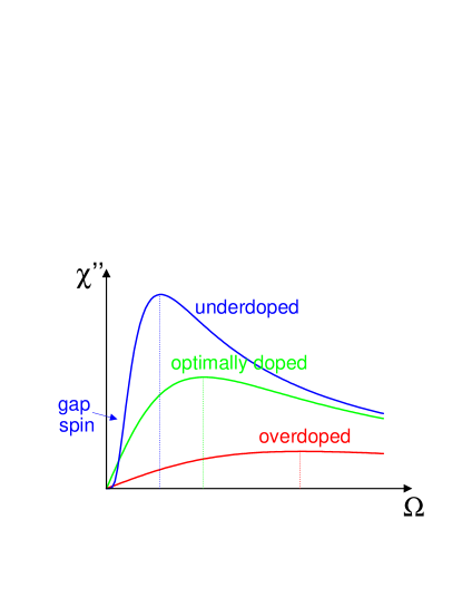
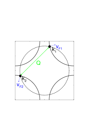
Figure 51: Left: Schematic behavior of the normal state spin susceptibility in cuprates. Normal state spin excitations in cuprates are overdamped. In underdoped cuprates a spin-gap effect additionally comes into play. Right: The hot spots are connected by a wavevector ${\bf Q}=(\pi,\pi)$. The fermionic dispersions near the hot spots is determined by the corresponding Fermi velocities ${\bf v}_{F1}$ and ${\bf v}_{F2}$.

Writing the susceptibility near the wavevector $Q=(\pi,\pi)$ as in Eq. (59),

$$\chi({\bf q},\Omega)=\frac{\chi_{Q}}{1+\xi^{2}({\bf q}-{\bf Q})^{2}-\bar{g}^{2}\chi_{Q}\Pi({\bf q},\Omega)}$$ (63)

the above form is obtained by evaluating the fermionic bubble. $\Gamma(\Omega)$ is then the imaginary part of the fermionic bubble times $\bar{g}^{2}$. The coupling constant $\bar{g}$ is related to $g$ by $3\bar{g}^{2}=g^{2}$. It is most easy to calculate the fermionic bubble $\Pi({\bf q},\Omega)$ at the hot spots, defined as the points on the Fermi surface connected by ${\bf Q}$. . The corresponding geometry is shown in Fig. 51 on the right, where the Fermi surface shifted by ${\bf Q}$ is shown as dashed line on top of the unshifted Fermi surface. Linearizing the dispersion around the hot spots and summing over all 8 hot spots results in [17, 290, 285]

$$\Gamma(\Omega)=\frac{4\bar{g}^{2}\Omega}{\pi v_{F}^{2}\sin 2\alpha}\;,$$ (64)

or, equivalently,

$$\Omega_{max}=\frac{\pi v_{F}^{2}\sin 2\alpha}{4\bar{g}^{2}\chi_{Q}}\;,$$ (65)

where $\alpha$ is the angle between the Fermi velocity at the hot spot and the wavevector ${\bf Q}$, and $v_{F}$ is the magnitude of the Fermi velocity at the hot spots. Near optimal doping in cuprates $\alpha\approx\pi/4$ so that $\sin 2\alpha\approx 1$. We obtain consequently the coupling constant via the formula

$$\bar{g}=\sqrt{\frac{\pi v_{F}^{2}\sin 2\alpha}{4\chi_{Q}\Omega_{max}}}$$ (66)

The parameters $v_{F}$, $\alpha$, $\Omega_{max}$ are all known from the normal state data from INS and ARPES. The value for $\chi_{Q}$ is not so well known for the normal state because the magnetic INS signal is very small. Thus, we follow Ref. [23] and extract the value from the superconducting state data.

In the superconducting state we can obtain a semi-phenomenological description of the resonance by using the same form Eq. (63) for the spin susceptibility in the superconducting state, with the superconducting state fermionic bubble $\Pi({\bf q},\Omega)$ now replacing the normal state one. Using the same approximation as above, as indicated in Fig. 52, one obtains a range in which the imaginary part of $\Pi$ is zero and the real part is given for small $\Omega$ in an expansion up to order $\Omega^{2}$ by,

$$\mbox{Re}\Pi({\bf Q},\Omega)=\frac{\Omega^{2}}{2v_{F}^{2}\Delta_{Q}}+\cdots$$ (67)

where $\Delta_{Q}$ is the gap magnitude on the hot-spot positions, and we assumed $\alpha=\pi/4$, which is a good approximations near the hot spots (however not near the nodes).

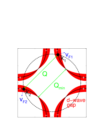
Figure 52: Fermi surface and scattering geometry in the superconducting state. The hot spots are connected by a wavevector ${\bf Q}=(\pi,\pi)$. The fermionic dispersions near the hot spots is determined by the corresponding Fermi velocities ${\bf v}_{F1}$ and ${\bf v}_{F2}$. The $d$-wave gap is indicated. The low-energy incommensurate wavevector ${\bf Q}_{min}$ is determined by node-node scattering.

Introducing this into the susceptibility, one obtains in this range $\Omega<2\Delta_{Q}$ the form

$$\chi({\bf Q},\Omega)\approx\frac{\chi_{Q}}{1-(\Omega/\Omega_{res})^{2}},$$ (68)

where in this approximation

$$\Omega_{res}=\sqrt{\frac{2v_{F}^{2}\Delta_{Q}}{\bar{g}^{2}\chi_{Q}}}=\sqrt{\frac{8\Omega_{max}\Delta_{Q}}{\pi}}\;.$$ (69)

In order to obtain the coupling constant separately from $\chi_{Q}$ we need the energy integrated weight of the resonance. The resonance contribution to the susceptibility is

$$\chi_{res}=\chi_{Q}\frac{\Omega_{res}^{2}}{\Omega_{res}^{2}-(\Omega+i0^{+})^{2}}\;,$$ (70)

and the weight of the resonance is then,

$$W_{res}=\int d\Omega\chi_{res}^{\prime\prime}({\bf Q},\Omega)=\frac{\pi}{2}\chi_{Q}\Omega_{res}$$ (71)

or solving for $\chi_{Q}$,

$$\chi_{Q}=\frac{2W_{res}}{\pi\Omega_{res}}\;.$$ (72)

The weight $W_{res}$ amounts to about 1.6 [94, 109, 89]. Knowing $\Omega_{res}$ very accurately from INS experiments, this allows to determine $\chi_{Q}$ as $\chi_{Q}\approx$13 eV${}^{-1}/$plane. Using this experimental $\chi_{Q}\sim 13$ eV^-1, $\Omega_{max}=20{\rm meV}$, and $v_{F}\sim 0.4{\rm eV}$ (in units where the lattice constant is 1) it follows that $\bar{g}\sim 1.75v_{F}\sim 0.7{\rm eV}$ [23].

The dimensionless coupling $\lambda$ can be extracted from the low-energy fermionic self-energy: $Re\Sigma(\epsilon)=-\lambda\epsilon$. $\Sigma({\bf k},\epsilon)$ is determined as 3$\bar{g}^{2}$ times a convolution of $\chi({\bf q},\Omega)$ with $G_{0}({\bf k}+{\bf q},\epsilon+\Omega)$. Again, linearizing the fermionic dispersion about the hot spots, and expanding $\chi$ quadratically around ${\bf Q}$ with a correlation length, $\xi$, it follows for the normal state that [285]

$$\lambda=\frac{3\bar{g}^{2}\chi_{Q}}{4\pi v_{F}\xi}=\frac{3v_{F}}{16\Omega_{max}\xi}$$ (73)

Substituting the above numbers and $\xi\sim 2$, we find $\lambda\sim 2$. Note that $\lambda$ refers here to fermions near the hot spots, and is obtained by coupling to the entire spin fluctuation spectrum. In the superconducting state, the part of $\lambda$ which is due to purely the spin resonance has been numerically obtained in Ref. [25], which was found to be $\sim 0.9$ at the $M$ point if the fermionic Brillouin zone for optimally doped materials. They also gave an approximate analytical formula for this weight,

$$\lambda_{M} \approx \frac{g^{2}I_{0}}{\pi}\cdot\frac{1}{(\Omega_{res}+E_{M})^{2}}+\frac{g^{2}w_{MN}}{\pi v_{N}v_{\Delta}}\frac{2}{\pi}\ln\left(1+\frac{\Delta_{A}}{\Omega_{res}}\right),$$ (74)

where $E_{M}=\sqrt{\xi_{M}^{2}+\Delta_{M}^{2}}$ is the quasiparticle binding energy at the $M$ point of the Brillouin zone, $w_{MN}$ the resonance intensity at the wavevector ${\bf q}_{MN}={\bf k}_{M}-{\bf k}_{N}$, $v_{N}=\partial_{k}\xi_{k}|_{k_{N}}$, $v_{\Delta}=\partial_{k}\Delta_{k}|_{k_{N}}$, and $\Delta_{A}$ is the superconducting gap at the antinodal Fermi surface point. For optimally doped Bi₂Sr₂CaCu₂O_8-δ they found the first term in this sum equal to $17.44I_{0}$ with $I_{0}=0.035$, which amounts to about 0.61, and the second term $\approx 0.21$, leading to a total of $\lambda_{M}\approx 0.82$. The spin-fluctuation continuum, not contained in this estimate, contributes the remaining part to the total coupling constant $\lambda\sim 2$ [25].

The such obtained value of $g$ is consistent with fitting resistivity data to spin fluctuation scattering [291, 292] and with Eliashberg calculations of $\Delta$ and $\Omega_{res}$ [22]. Such a large value of $g$ is also expected on microscopic grounds: in the Hubbard model, the effective $g$ is expected to be of the order of the fermionic bandwidth $W$ [293, 294] which is $1{\rm eV}$ for the cuprates [23]. The estimate $\lambda\sim 2$ is consistent with the velocity renormalization estimated from normal state ARPES experiments [142], and with the bare density of states extracted from the specific-heat data of Ref. [295]. It was shown by Abanov et al. [285] that spin fluctuations are slow compared to fermions, and for that reason an “effective” Migdal theorem exists for fermions near the hot spots, which justifies the use of the above perturbation theory.

The above picture of the spin resonance and its effect on fermions has been challenged by a number of authors. Kee et al. [286] argued that $g\sim 14{\rm meV}$ and $\lambda\sim 10^{-3}$, two and three orders of magnitude smaller than the values above, respectively. However, the discrepancy can be attributed to different definitions of the effective coupling constants in the different theories. In the low-doping regime, where the Fermi surface evolves toward small hole pockets, fermions couple to antiferromagnetic magnons [23]. In this case, the spin mode couples to fermions only through gradients, i.e., the renormalized coupling $g_{eff}$ is much smaller than $g$. This reduction from $g$ to $g_{eff}$ is the result of strong vertex corrections if antiferromagnetic magnons are present in the normal state [296, 297, 298], and occurs because antiferromagnetic magnons are only compatible with a small Fermi surface (hole pockets), in which case $g$ has been absorbed into the definition of renormalized fermions with a spin density wave energy gap [8, 299]. Here we are dealing, however, with the metallic phase where a large Fermi surface exists, and where the normal state spin dynamics is purely relaxational. In this case, $g$ is the appropriate coupling to use, not $g_{eff}$.

To summarize, the large intensity of the resonance at ${\bf Q}=(\pi,\pi)$ is consistent with the small value of the total momentum and frequency integrated intensity of the resonance peak, and also with the fact that the magnetic part of the condensation energy is only a small fraction of $J$ [23]. The spin-fermion coupling $g$ is of the order of $1{\rm eV}$ and this value of $g$ is consistent with experiment. This $g$ is sufficiently large that scattering from the resonance can substantially affect the electronic properties of the cuprates below $T_{c}$.

4.2 Theoretical model

As we are interested in the renormalization of the fermionic dispersion as a result of the coupling of electrons to the sharp magnetic-fluctuation mode at low energies, we search for a minimal model which captures the low-energy physics correctly. Such a model was suggested in Refs. [24, 25]. The idea there is to concentrate on the superconducting state assuming that superconducting order is already established without coupling to this resonant feature in the spin-fluctuation spectrum. Thus, the superconducting state is described by an independent order parameter $\Delta_{k}$. The origin of the superconducting pairing instability can be for example the spin fluctuations continuum, which extends to high energies, or other sources. The pairing problem is assumed to be of BCS type. The spin fluctuation resonance supports pairing, but does not cause superconductivity in and of itself [7, 25, 23]. Although semi-phenomenological, this approach has the advantage that the conclusions drawn are independent on the specific microscopic pairing mechanism.

The order parameter is chosen to have $d$-wave symmetry (here and in the following the unit of length is the lattice constant $a$),

$$\Delta_{k}=\frac{\Delta_{M}}{2}(\cos k_{x}-\cos k_{y}).$$ (75)

In agreement with the experiments of [174] it is assumed that in the case of bilayer materials the pairing interaction has no interplane contribution. The magnitude $\Delta_{M}$ is determined by the peak position of the ARPES spectrum at the $M$ point after including self-energy effects due to coupling to the spin fluctuations. The coupling to the resonant spin-fluctuation mode leads in general to a renormalization of the gap, and it is this renormalized gap which is observed in experiments.

The model can be formulated in terms of retarded Green functions, $G^{R}_{\epsilon,k}$, for fermionic excitations in the superconducting state. These Green functions are functionals of the normal state electronic dispersion $\xi_{k}$, the order parameter $\Delta_{k}$, and the self energies due to coupling to spin fluctuations, $\Sigma^{R}_{\epsilon,k},\Phi^{R}_{\epsilon,k}$. The ‘normal state’ refers here to the state at the same temperature, but with zero order parameter.

4.2.1 Tight binding fit to normal state dispersion

In order to model the normal-state properties as realistic as possible the electronic dispersion $\xi_{k}$ is obtained from ARPES experiments in the normal state, and parameterized by using a six parameter tight binding fit of the form

$$\xi_{k} = t_{0}+t_{1}\frac{\cos k_{x}+\cos k_{y}}{2}+t_{2}\cos k_{x}\cos k_{y}+t_{3}\frac{\cos 2k_{x}+\cos 2k_{y}}{2}$$ (76)

$$+t_{4}\frac{\cos 2k_{x}\cos k_{y}+\cos k_{x}\cos 2k_{y}}{2}+t_{5}\cos 2k_{x}\cos 2k_{y}\;.$$

The six parameters $t_{0}-t_{5}$ are conveniently determined by using characteristic features in the experimentally measured electronic normal-state dispersion.

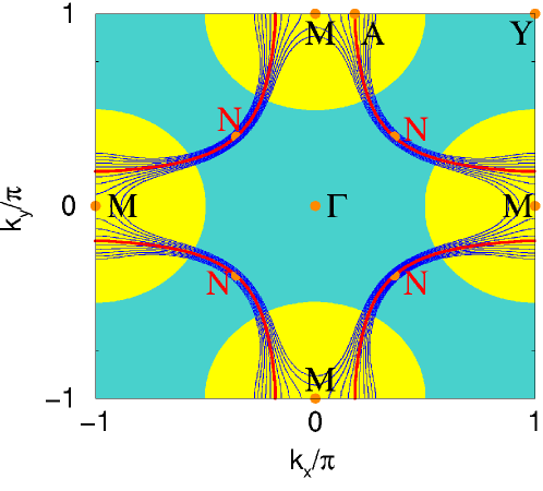
Figure 53: Equal energy contours around the Fermi surface shown as thin curves for energies between $\pm 50$meV. The Fermi surface is shown as a thick curve. The dispersion used here was obtained by a 6-parameter tight binding fit to angle resolved photoemission dispersions in optimally doped Bi₂Sr₂CaCu₂O_8-δ [7]. The dispersion has a saddle point at the $M$ point. The $N$ point corresponds to the node of the $d$-wave order parameter in the superconducting state. Two characteristic regions can be defined: the regions around the $M$ points (light) as opposed to the remaining region which includes the $N$ points.

The six features employed in Ref. [25] are the positions of the $N$ (node) and $A$ (antinode) points in Fig. 53, parameterized by $k_{\Gamma N}=|{\bf k}_{N}-{\bf k}_{\Gamma}|$ and $k_{MA}=|{\bf k}_{A}-{\bf k}_{M}|$, the band energies at the $M$ and $Y$ points, $\xi_{M}$ and $\xi_{Y}$, the Fermi velocity at the $N$ point, $v_{N}=|{\bf v}_{N}|$, and the inverse effective mass along direction $M-\Gamma$ at the $M$ point, $m_{M}^{-1}$. Table 4.2.1 shows as example the parameters appropriate for optimally doped Bi₂Sr₂CaCu₂O_8+δ (OP Bi2212) [25]. The Fermi surface for such a tight binding fit and corresponding equal-energy contours in the range between $\pm$50 meV are shown in Fig. 53. In this Figure we indicate a separation of the Brillouin zone into two types of regions. The areas around the $M$ points are dominated by the flat dispersion near the saddle point, which introduces a new energy scale given by the distance of the saddle-point singularity from the chemical potential. In the remaining region, which includes the nodes of the order parameter, the dispersion is steep in the direction perpendicular to the Fermi surface, and excitations are restricted to the close vicinity of the Fermi surface.

The parameter $\xi_{Y}$ in the tight binding dispersions is in principle not known from experiment. However, as the high-energy dispersion is not important for the low-energy physics (except for an energy independent contribution to the quasiparticle renormalization factor), it can be set to a reasonable value to preserve the overall dispersion shape as observed from experiment. On a formal level, it is always possible to introduce a high-energy contribution to the quasiparticle renormalization factor in such a way that it accounts for the true high-energy dispersion.

The inverse mass at the $M$ point is known to be negative and small in the $M-\Gamma$ direction, and it was suggested that it could be zero, giving rise to an extended van Hove singularity [160, 158]. The inverse effective mass decreases when coupling to the spin fluctuation mode is taken into account, and it is this renormalized inverse mass which is experimentally observed.

Similarly, the value of the Fermi velocity at the node is renormalized by self-energy effects to moderately smaller values. Again, it is these renormalized value of the Fermi velocity which is observed in experiment. The parameters most sensitive to doping variations are $\xi_{M}$ and ${\bf k}_{A}$.

For the case of a bilayer splitting, we parameterize the Fermi surface by the same six parameters plus the bilayer splitting between bonding ($b$) and antibonding ($a$) band. If the bonding and antibonding dispersions are written as $\xi_{k}^{(b)}$ and $\xi_{k}^{(a)}$, the resulting energy splitting is anisotropic [166, 188]:

$$\xi_{k}^{(a)}-\xi_{k}^{(b)}=\frac{1}{2}t_{\perp}(\cos k_{x}-\cos k_{y})^{2}.$$ (77)

The normal state dispersion for both bands is then determined by a total of seven parameters. An example, appropriate for overdoped Bi₂Sr₂CaCu₂O_8+δ (OD Bi2212), and used in Ref. [24], is presented in Table 4.2.1.

Parameters for the effective dispersion $\xi_{k}$ ([25, 24]). BB and AB in the second line refers to bonding band and antibonding band. OP and OD Bi2212 stand for optimally doped and overdoped Bi₂Sr₂CaCu₂O_8+δ. $k_{\Gamma N}a$ $k_{MA}a$ $\xi_{M}$ $\xi_{Y}$ $\hbar v_{N}/a$ $\hbar^{2}/m_{M}a^{2}$ OP Bi2212 [25] $-$ 0.36$\sqrt{2}\pi$ 0.18$\pi$ $-34$ meV 0.8 eV 0.6 eV $-0.2376$ eV OD Bi2212 [24] BB 0.37$\sqrt{2}\pi$ 0.217$\pi$ $-105$ meV 0.8 eV 0.6 eV $-$ AB 0.135$\pi$ $-18$ meV $-$

As mentioned above, the normal state dispersion $\xi_{k}$, and also the order parameter $\Delta_{k}$, are phenomenological quantities, which are already renormalized by other effects which we do not need to specify, but which are assumed to influence the physics only on an energy scale large compared to the scale of interest (50-100 meV). The self energies due to spin fluctuations will have a part due to the particle-hole continuum, and another part due to the resonance. In general it is necessary to include both parts of the spectrum. However, for the low-energy region below 100 meV it is possible to study a simplified model, in which the effect of the continuum part of the spin fluctuation spectrum is included by a constant renormalization of the normal state dispersion and the order parameter [25]. In this case the main physics is dominated by the coupling of the electrons to the resonant spin fluctuations. The ‘normal state’ reference is here defined as the state with zero order parameter, interacting with a spin fluctuation spectrum having no resonance part and a continuum part identical to that in the superconducting state. This is different from the physical normal state, because the spin fluctuation continuum changes when going from the normal to the superconducting state, leading to an additional renormalization of the dispersion.

At higher energies, the spin fluctuation continuum can be excited, and this leads to an additional strong fermionic damping. The appropriate model to study this effect is the extended model which explicitly includes the gapped spin fluctuation continuum. For this extended model, the ‘normal state’ dispersion has a different renormalization factor as compared to the simple model above. The dispersions in Table 4.2.1 are the appropriate dispersions for the simplified model. For the extended model it is to be scaled and shifted back in energy (so that the energy of the van Hove singularity closest to the $M$ point stays at its original value) as described below in more detail [24, 25].

4.2.2 Model spectrum and basic equations

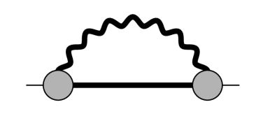
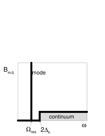
Figure 54: Left: Self energy for electrons (full lines). The wavy line denotes a spin fluctuation. Right: the model spin fluctuation spectrum we used for the wavy line in the Feynman diagram. The mode affects the low energy fermionic properties. The continuum part only couples to electrons with higher energies, and is neglected in the simple form of the model [7]. Damping of electrons at energies above 100 meV is caused by the continuum part, and is included in the extended model [25]. (From Ref. [25], Copyright ©2003 APS).

It is found that all essential features of the self-energy effects in the superconducting state are obtained using a minimal model with a spin fluctuation spectrum shown in Fig. 54 [25]. The self energy is given by the diagram in Fig. 54 on the left, and its retarded part is written within standard Keldysh technique as,

$$\Sigma^{R}_{\epsilon,k}=\frac{i}{2}\sum_{q,\omega}\left(G^{R}_{\epsilon-\omega,k-q}g^{2}D^{K}_{\omega,q}+G^{K}_{\epsilon-\omega,k-q}g^{2}D^{R}_{\omega,q}\right),$$ (78)

where $D=-\chi$ is the bosonic propagator, $G$ the fermionic propagator, and $g$ the coupling constant between the two. Analogously, in the superconducting state the anomalous (off-diagonal) self energy is obtained from

$$\Phi^{R}_{\epsilon,k}=\frac{i}{2}\sum_{q,\omega}\left(F^{R}_{\epsilon-\omega,k-q}g^{2}D^{K}_{\omega,q}+F^{K}_{\epsilon-\omega,k-q}g^{2}D^{R}_{\omega,q}\right),$$ (79)

with the anomalous fermionic propagator $F$. In equilibrium, the Keldysh components are given by the expressions

$$D^{K}_{\omega,q} = \left(D^{R}_{\omega,q}-D^{A}_{\omega,q}\right)\coth\frac{\omega}{2T}=-iB_{\omega,q}(1+2b_{\omega}),\quad$$ (80)

$$G^{K}_{\epsilon,k} = \left(G^{R}_{\epsilon,k}-G^{A}_{\epsilon,k}\right)\tanh\frac{\epsilon}{2T}=-iA_{\epsilon,k}(1-2f_{\epsilon}),\quad$$ (81)

$$F^{K}_{\epsilon,k} = \left(F^{R}_{\epsilon,k}-F^{A}_{\epsilon,k}\right)\tanh\frac{\epsilon}{2T}=-iC_{\epsilon,k}(1-2f_{\epsilon}),\quad$$ (82)

where $B_{\omega,q}=-2$Im$D^{R}_{\omega,q}$ and $A_{\epsilon,k}=-2$Im$G^{R}_{\epsilon,k}$ are the bosonic and fermionic spectral functions, and $b_{\omega}$, $f_{\epsilon}$ their corresponding distribution functions, respectively. Note, that the Keldysh components $G^{K}$ and $D^{K}$ are purely imaginary. For the anomalous propagator, the function $C_{\epsilon,k}=i(F^{R}_{\epsilon,k}-F^{R}_{-\epsilon,-k})=-C_{-\epsilon,-k}$ is only real in the case of a real gauge (real order parameter).

The spectral function for the spin-fluctuation spectrum in Fig. 54 is the sum between the resonance part and the continuum part,

$$g^{2}B_{\omega,q}=g^{2}B^{r}_{\omega,q}+g^{2}B^{c}_{\omega,q}.$$ (83)

with a resonance part sharp in energy,

$$g^{2}B^{r}_{\omega,q}=2g^{2}w_{q}\left[\delta(\omega-\Omega_{res})-\delta(\omega+\Omega_{res})\right]$$ (84)

and a continuum with onset at $2\Delta_{h}$,

$$g^{2}B^{c}_{\omega,q}=2g^{2}c_{q}\left[\Theta(\omega-2\Delta_{h})-\Theta(-\omega-2\Delta_{h})\right]\;.$$ (85)

This form for the gapped continuum is similar to the gapped marginal Fermi liquid spectrum considered in Refs. [192, 16].

In order for the real part of the self energy to converge, the continuum has to be cut-off at high energies. The precise form of this high-energy cut-off is irrelevant for the low-energy part of the fermionic Green function, and variation of the cut-off leads to only a weakly energy-dependent contribution to the renormalization factor which can be absorbed in the dispersion $\xi_{k}$ as described above. Thus, any change in the high-energy behavior of the continuum spectrum is accounted for by a redefinition of the quasiparticle renormalization factor. The energy width of the resonance can be assumed in very good approximation as zero, as was shown in Ref. [25].

We assume in Eq. (84) that the resonance energy is independent on momentum. Strictly speaking, this is not true, as the resonance is part of a dispersive incommensurate response as shown in Fig. 8. However, as can be seen from Fig. 49, in particular on the left, which is for Bi₂Sr₂CaCu₂O_8+δ, the weight of the incommensurate response is very quickly reduced when moving away from the resonance frequency $\Omega_{res}$. Thus, the approximation of a dispersionless mode is a very good one.

The momentum dependences of the resonance mode and the continuum, are given by the functions $w_{q}$ and $c_{q}$,

$$w_{q} = \frac{w_{Q}}{1+4\xi_{sfl}^{2}(\cos^{2}\frac{q_{x}}{2}+\cos^{2}\frac{q_{y}}{2})},$$ (86)

$$c_{q} = \frac{c_{Q}}{1+16\xi_{c}^{4}(\cos^{4}\frac{q_{x}}{2}+\cos^{4}\frac{q_{y}}{2})}(1+\beta)-c_{Q}\beta,$$ (87)

where $\xi_{sfl}$ is the correlation length of the resonance and $\xi_{c}$ that of the gapped continuum. The momentum dependence of the continuum takes into account the experimentally observed flatter behavior around the $(\pi,\pi)$ wavevector at higher energies. The parameter $\beta$ is chosen in such a way that $c_{q}$ is zero at ${\bf q}=0$, and is introduced such that the response far away from the $(\pi,\pi)$ wavevector is small, as experimentally observed. The functions $w_{q}$ and $c_{q}$ are plotted in Fig. 55.

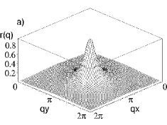
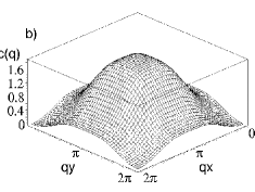
Figure 55: Momentum dependence of a) the resonance mode and b) the gapped spin fluctuation continuum. The resonance mode is peaked at ${\bf Q}=(\pi,\pi)$ with a correlation length equal to twice the lattice constant, $\xi_{res}=2a$. The continuum spectrum, in contrast, is rather broad around ${\bf Q}$. (From Ref. [24], Copyright ©2002 APS).

The resonance mode, shown in Fig. 55a, is peaked at ${\bf Q}$, with a correlation length of $\xi_{res}=2a$, where $a$ is the lattice constant. The gapped continuum, shown in Fig. 55b, is much broader. This is motivated by the experimental data [94], which show that the continuum is enhanced around ${\bf Q}$ with a correlation length of only 0.5 lattice constants. Also, the momentum dependence of the continuum excitations exhibit experimentally a flat behavior around ${\bf Q}$, as in Fig. 55b. To simplify the model, we use the same functional form for the gapped continuum in the even and odd scattering channels. This is consistent with the superconducting state data, where the gap in the odd channel (about twice the maximal superconducting gap), is close to the optical gap in the even channel (see Fig. 10).

The retarded Green function as a function of the self energies is given as usually by,

$$G^{R}_{\epsilon,k}[\Sigma^{R}_{\epsilon,k},\Phi^{R}_{\epsilon,k}] = \frac{Z_{\epsilon,k}\epsilon+\bar{\xi}_{\epsilon,k}}{(Z_{\epsilon,k}\epsilon+i0^{+})^{2}-E_{\epsilon,k}^{2}},$$ (88)

$$F^{R}_{\epsilon,k}[\Sigma^{R}_{\epsilon,k},\Phi^{R}_{\epsilon,k}] = \frac{\bar{\Delta}_{\epsilon,k}}{(Z_{\epsilon,k}\epsilon+i0^{+})^{2}-E_{\epsilon,k}^{2}},$$ (89)

with excitation energies

$$E_{\epsilon,k}=\sqrt{\bar{\xi}_{\epsilon,k}^{2}+\bar{\Delta}_{\epsilon,k}\bar{\Delta}_{-\epsilon,-k}^{\ast}}\;.$$ (90)

The renormalized dispersion and gap function are given in terms of the diagonal ($\Sigma^{R}_{\epsilon,k}$) and off-diagonal ($\Phi^{R}_{\epsilon,k}$) in particle-hole space self energies, as

$$\bar{\xi}_{\epsilon,k} = \xi_{k}+\frac{\Sigma^{R}_{\epsilon,k}+\Sigma^{R\ast}_{-\epsilon,-k}}{2}\qquad\bar{\Delta}_{\epsilon,k}=\Delta_{k}+\Phi^{R}_{\epsilon,k},$$ (91)

and the renormalization function as

$$Z_{\epsilon,k} = 1-\frac{\Sigma^{R}_{\epsilon,k}-\Sigma^{R\ast}_{-\epsilon,-k}}{2\epsilon}$$ (92)

The self energies $\Sigma^{R}_{\epsilon,k}$ and $\Phi^{R}_{\epsilon,k}$ are even in momentum, and for $\Phi^{R}_{\epsilon,k}$ the additional symmetry $\Phi^{R}_{\epsilon,k}=\Phi^{R\ast}_{-\epsilon,-k}$ holds (we use a real gauge for the order parameter $\Delta_{k}$). The coupling constant $g$ between electrons and the spin fluctuation spectrum is assumed to be independent of energy and momentum.

Although the self-energy Eq. (78) is generally correct also in non-equilibrium, it is advantageous in the case of equilibrium to rewrite the expression. In equilibrium it is possible to make use of the identity

$$\sum_{\omega}D^{R}_{\omega}G^{K}_{\epsilon-\omega} = -i\sum_{\omega}\tanh\frac{\epsilon-\omega}{2T}B_{\omega}G^{R}_{\epsilon-\omega}$$ (93)

$$+\sum_{\omega}\left(D^{A}_{\omega}G^{R}_{\epsilon-\omega}-D^{R}_{\omega}G^{A}_{\epsilon-\omega}\right)\tanh\frac{\epsilon-\omega}{2T}\;,$$

and to convert the second line of Eq. (93) into a Matsubara sum by noting that $D^{A}_{\omega}G^{R}_{\epsilon-\omega}$ is an analytic function in the lower $\omega$ half plane, and analogously $D^{R}_{\omega}G^{A}_{\epsilon-\omega}$ analytic in the upper half plane. An analogous formula holds for $\sum_{\omega}D^{R}_{\omega}F^{K}_{\epsilon-\omega}$. The self energies are then given in terms of the spectral function of the spin fluctuations with energy $\omega$ and momentum ${\bf q}$, $B_{\omega,q}$, by the expressions [300]

$$\Sigma^{R}_{\epsilon,k} = \sum_{\omega,q}(b_{\omega}+f_{\omega-\epsilon})g^{2}B_{\omega,q}G^{R}_{\epsilon-\omega,k-q}-T\sum_{\epsilon_{n},q}G^{M}_{k-q}(i\epsilon_{n})g^{2}D^{M}_{q}(\epsilon-i\epsilon_{n})\quad$$ (94)

$$\Phi^{R}_{\epsilon,k} = \sum_{\omega,q}(b_{\omega}+f_{\omega-\epsilon})g^{2}B_{\omega,q}F^{R}_{\epsilon-\omega,k-q}-T\sum_{\epsilon_{n},q}F^{M}_{k-q}(i\epsilon_{n})g^{2}D^{M}_{q}(\epsilon-i\epsilon_{n}),\quad$$ (95)

where $G^{M}$, and $D^{M}$ are the fermionic and bosonic Matsubara Green functions. Analogously, $F^{M}$ is the anomalous Matsubara Green function. The Matsubara sums in Eqs. (94) and (95) only contribute to the real part of the self energies. The representations (94) and (95) are a bit unconventional, however for finite temperatures very convenient. Note that for optimally and overdoped materials unrenormalized Green functions can be used in Eqs. (94)-(95) [24, 25]. This approximation is sufficient to explain a large variety of data, and can be justified by considerations discussed in Ref. [294].

The function $b_{\omega}+f_{\omega-\epsilon}$ as a function of $\omega$ for fixed $\epsilon$ is at zero temperature nonzero only between $\omega=0$ and $\omega=\epsilon$, and is equal to sign$(\epsilon)$ in this range. This ’box function’ is smeared out at finite temperatures by the amount of the thermal energy $k_{B}T$. However, because the spin-fluctuation spectrum is gapped by much more than the thermal energy in the superconducting state, for all practical reasons $b_{\Omega_{res}}=0$ holds. Thus, thermally excited modes can be safely neglected, and only emission processes at the resonant mode energy are relevant. Furthermore, for any gapped spin-fluctuation spectrum with gap $\Omega$, the first terms in Eq. (94) and (95) are negligible in the range $-\Omega<\epsilon<\Omega$ (apart from temperature smearing near the value $\pm\Omega$). Thus, assuming that the spin fluctuation spectrum is gapped below the resonance energy, at zero temperature scattering of electronic excitations is disallowed in the interval $-\Omega_{res}<\epsilon<\Omega_{res}$. This is an expression of the fact that at least an energy $\Omega_{res}$ must be spent in order to emit one spin fluctuation mode. This is the case for optimally and overdoped cuprates. For strongly underdoped cuprates, scattering is disallowed only in the range $-E_{g}<\epsilon<E_{g}$, where $E_{g}$ is the spin gap which is smaller than $\Omega_{res}$. Also, as an implication, the renormalization function, determined by the real part of the self energy, is given in the low energy range by the second terms of Eqs. (94) and (95) only (but also has contributions from the first terms for higher energies).

4.3 Contribution from the spin fluctuation mode

For a sharp bosonic mode the spectral function is given by Eq. (84) with the energy integrated weight given by Eq. (86). The mode is enhanced at the ${\bf Q}=(\pi,\pi)$ point with a correlation length $\xi_{sfl}$. It is a good approximation to assume the mode as perfectly sharp in energy [25]. From neutron scattering data obtained on Bi₂Sr₂CaCu₂O_8+δ, the energy integrated weight of the resonance mode was determined as 1.9 $\mu_{B}^{2}$ [99], leading (after dividing out the matrix element $2\mu_{B}^{2}$) to $w_{Q}=0.95$. We fit ARPES data near optimal doping [7], giving $g^{2}w_{Q}=0.4$eV². This implies that the coupling constant is equal to $g=0.65$ eV. This is a reliable value as discussed in [23]. In Table 4.3, the minimal parameter set for optimally doped compounds is presented (from the band structure tight binding fit, only the parameter $\xi_{M}$ is listed as the results are insensitive to reasonable variations of the other parameters)

Minimal parameter set appropriate for optimally doped Bi₂Sr₂CaCu₂O_8+δ. $\Delta_{M}$ $\Omega_{res}$ $\xi_{M}$ $\xi_{sfl}$ $g^{2}w_{Q}$ 35 meV 39 meV $-34$ meV 2$a$ 0.4 eV²

In the following sections we review results for numerical calculations at finite temperatures obtained from solving Eqs. (94)-(95) using bare Green functions on the right hand side. However, for better understanding of the results it will be convenient to also discuss the zero-temperature limit. Using bare Green functions, the self energy at zero temperature can be written as

$$\mbox{Im}\Sigma^{R}_{\epsilon,k} = -\sum_{q}g^{2}w_{q}A^{-}_{k-q}\delta(\epsilon+\Omega_{res}+E_{k-q})$$ (96)

$$-\sum_{q}g^{2}w_{q}A^{+}_{k-q}\delta(\epsilon-\Omega_{res}-E_{k-q})$$

$$\mbox{Re}\Sigma^{R}_{\epsilon,k} = -\sum_{q}\frac{g^{2}w_{q}}{\pi}\cdot\frac{\epsilon+\left(1+\frac{\Omega_{res}}{E_{k-q}}\right)\xi_{k-q}}{(\Omega_{res}+E_{k-q})^{2}-\epsilon^{2}}$$ (97)

where $E_{k}=\sqrt{\xi_{k}^{2}+|\Delta_{k}|^{2}}$, $A^{\pm}_{k}=(1\pm\xi_{k}/E_{k})/2$. For negative energies, only the first sum in Eq. (96) is nonzero. The sum is a weighted average of the expression $A^{-}_{k-q}\delta(\epsilon+\Omega_{res}+E_{k-q})$ with weight factors $w_{q}$. For given fermion energies, $\epsilon$, and momenta, ${\bf k}$, the delta function restricts the allowed spin fluctuation momenta ${\bf q}$. Similar zero temperature formulas hold for the off diagonal self energy,

$$\mbox{Im}\Phi^{R}_{\epsilon,k} = -\sum_{q}g^{2}w_{q}\frac{\Delta_{k-q}}{2E_{k-q}}\Big{[}\delta(\epsilon-\Omega_{res}-E_{k-q})-\delta(\epsilon+\Omega_{res}+E_{k-q})\Big{]}\quad$$ (98)

$$\mbox{Re}\Phi^{R}_{\epsilon,k} = -\sum_{q}\frac{g^{2}w_{q}}{\pi}\cdot\frac{\left(1+\frac{\Omega_{res}}{E_{k-q}}\right)\Delta_{k-q}}{(\Omega_{res}+E_{k-q})^{2}-\epsilon^{2}}.$$ (99)

4.3.1 Characteristic electronic scattering processes

Scattering of electrons via emission of a magnetic resonance excitation is characterized by several important peculiarities. They are a result of the interplay between kinetic scattering restrictions due to the Pauli principle for electrons and the restriction of the resonance momentum to the near vicinity of the ${\bf Q}=(\pi,\pi)$ wavevector. The kinetic restrictions for electronic scattering are given by the fact that low-energy scattering is restricted to a close vicinity of the Fermi surface. In the present case the electron scattering processes can involve the emission of a resonance mode with energy $\Omega_{res}$. However, the electrons also acquire a large momentum ${\bf q}\sim\pm(\pi,\pm\pi)$ from the scattering event, which leads to a strongly anisotropic scattering rate.

The scattering rate of electrons is determined by the imaginary part of the self energy, which can be extracted from photoemission spectra. In a photoemission experiment a photon with energy $h\nu$ creates a photo-hole below the chemical potential and the energy $\epsilon$ and momentum ${\bf k}$ of the electron emitted from the sample is detected. The resulting spectra give information about the spectrum of a hole interacting with the collective excitations present in the solid. The creation of such a photohole can be either direct or can be accompanied by the simultaneous creation of collective excitations, which for the case of the spin-1 resonance mode we consider have a sharp energy $\Omega_{res}$ and a momentum not too far away from ${\bf Q}=(\pi,\pi)$. The detection of the emitted electron at a certain momentum ${\bf k}$ will lead to a ‘coherent peak’ from the creation of photoholes without additional collective excitations, and a broad incoherent continuum from the creation of photoholes accompanied by the creation of additional collective excitations. The latter has a broad distribution due to the momentum spread of the resonant magnetic excitations, and this distribution will be gapped by at least the mode energy, because the highest possible energy the emitted electron can have in this case is that of the chemical potential minus the mode energy. The peak determines the binding energy of the well defined fermionic excitations in the system (quasiholes).

The probability to create a photohole without creating magnetic excitations is small for a hole near the $M$ point of the Brillouin zone, because of the large number of states present near the chemical potential at momenta $(\pi,\pi)$ away (again corresponding to $M$-symmetry points of the Brillouin zone). In fact, the area of the flat dispersion region is large enough to exhaust almost the entire weight of the magnetic resonance during scattering events. Thus, the peak intensity will be reduced there, and the broad loss spectrum at higher energies due to emission of collective spin-1 modes is strong. Near the nodal points, the probability to create a photohole without additionally exciting magnetic collective excitations is high, thus the peak intensity is strong here and the incoherent loss spectrum due to collective spin-1 modes is small (there will be a considerable incoherent part due to the spin-fluctuation continuum though; this will be discussed later).

From the above it is clear that three effects are contributing to the physics of the low-energy scattering events: the peaked behavior in momentum of the magnetic resonance, the fact that scattering events take place only between points near the chemical potential, and the presence of a large number of states near the $M$ point of the Brillouin zone.

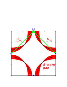
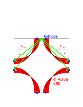
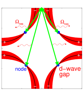
$-\Omega_{res}-E_{M}$

$-\Omega_{res}-\Delta_{A}$

$-\Omega_{res}$

Figure 56: The relevant scattering processes for an electron removed from the $M$ point. They correspond to the characteristic energies: $-(\Omega_{res}+E_{M})$ (left), $-(\Omega_{res}+\Delta_{A})$ (middle), and $-\Omega_{res}$ (right). The corresponding energies for an injected electron have opposite sign. The magnitude of the $d$-wave order parameter is indicated as shading around the Fermi surface.

There are three characteristic frequencies which determine the onset and maxima of scattering, and which will show up in the imaginary part of the self energy, discussed in the following section. They are shown for the case of an injected hole (removed electron) at the $M$ point of the Brillouin zone in Fig. 56. The first, shown in Fig. 56 on the right, determines the onset of scattering in the superconducting state at energy $\epsilon=-\Omega_{res}$, which is connected with the fact that it costs a minimal energy $\Omega_{res}$ to emit a resonant excitation. The important scattering vectors are here the wavevectors connecting the nodes with the $M$ points of the Brillouin zone, ${\bf q}=({\bf k}_{M}-{\bf k}_{N})$ mod $({\bf G})$ (${\bf G}$ denotes a reciprocal lattice vector). Below this onset energy, the imaginary part of the considered electronic self-energy is zero at $T=0$ (at finite temperatures this onset is smoothened on the temperature scale). When taking into account the incommensurate spin-fluctuations at lower energies, a small finite contribution to the imaginary part of the self energy will be present also below this onset energy. As the phase space for final scattering states near the nodes is very small, and in addition the wavevector for scattering from $(\pi,0)$ to the nodal point does not match the antiferromagnetic wavevector, the magnitude of scattering near the onset is small as well.

The first maximal effect of scattering with increasing binding energy is reached when the final scattering states are at the antinodal points, where the dispersion in the superconducting state has an extremal point. This corresponds to Fig. 56 middle. The relevant scattering wavevectors are ${\bf q}=({\bf k}_{M}-{\bf k}_{A})$ mod $({\bf G})$, and electrons are scattered strongly between the $M$ point and the $A$ points, and the characteristic energy of these scattering events is the sum of the energy of the emitted mode and the binding energy at the $A$ point, $\epsilon=-(\Omega_{res}+\Delta_{A})$.

A third special point is reached when the binding energy increases even more to the value $\epsilon=-(\Omega_{res}+E_{M})$ (with $E_{M}=\sqrt{\xi_{M}^{2}+\Delta_{M}^{2}}$), at which scattering events between the $M$ points involving spin fluctuations with momentum ${\bf q}={\bf Q}$ (and with ${\bf q}={\bf 0}$) are allowed. This corresponds to Fig. 56 left. At this wavevector the intensity of the magnetic mode is maximal, and the number of final scattering states is strongly increased due to the flat dispersion near the $M$ points. Both facts lead to a very strong scattering at this particular binding energy for quasiparticles near the $M$ point of the Brillouin zone.

At even higher binding energies the gapped continuum part of the bosonic spectrum becomes involved, and this region will be discussed later. For the parameter set of Table 4.3, corresponding to optimal doping, the characteristic energies are: $\Omega_{res}=39$ meV, $\Omega_{res}+\Delta_{A}=71.2$ meV, and $\Omega_{res}+E_{M}=87.8$ meV. The energy range in which the scattering is maximal is between 70 and 90 meV. In this range also the strongest renormalization effects are expected.

4.3.2 Electronic self energy

The self energy has a characteristic shape as a function of energy, which is conserved qualitatively for all points in the Brillouin zone. This is a consequence of the fact that all points are coupled via the spin fluctuation mode, which has a finite width in momentum, to all special points in the Brillouin zone with their corresponding characteristic energies. These special points are the nodal $N$ points, and the van Hove singularities at the $M$ points and the $A$ points (the latter is a dispersion maximum in the superconducting state). Because the general shape of the energy dependence of the self energy does not vary much with momentum (although the overall intensity does), it is sufficient to discuss the important features in the energy dependence of the self energy at the $M$ point.

In Fig. 57, the results for the electronic self energy at the $M$ point of the Brillouin zone are shown as a function of energy.

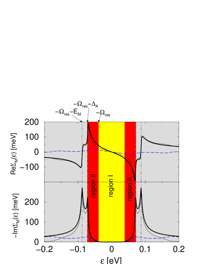
Figure 57: Mode contribution to the real and imaginary part of the electronic self energy at the $M$ point, numerically evaluated using a broadening parameter $\delta=$ 1 meV. Characteristic energies are indicated. Electrons at low temperatures are scattered only if their energy is larger than $\Omega_{res}$, so that they are able to emit a collective-mode excitation. As dashed curves the nodal contributions, when restricting the quasiparticle momenta to the regions outside the area around the $M$ points discussed in the text, is shown. The thin dotted curves are the contribution when restricting the quasiparticle momenta to the regions inside the area around the $M$ points. The parameters used are: $T=40$K, $\Omega_{res}=$39 meV, $\Delta_{M}=$35 meV. (After Ref. [25], Copyright ©2003 APS).

The three characteristic energies discussed in section 4.3.1 can be readily read off from Fig. 57. They define two characteristic regions.

In region I the scattering rate for scattering of electrons or holes with the magnetic mode is zero at zero temperature (this statement is true for electrons at any point in the Brillouin zone). A finite temperature affects only the onset region, as $k_{B}T<<\Omega_{res}$. Concentrating in the following on the hole spectrum (negative energies), the onset at $\epsilon=-\Omega_{res}$ is determined by the coupling to nodal electrons via emission of a spin fluctuation mode. The real part of the self energy is rather linear in region I.

In region II, a larger and larger area around the nodes participates in scattering events, until finally the point at the zone boundary with maximal gap, $\pm\Delta_{A}$, is reached. In Fig. 57 we also show as dotted curves the contribution to the electron scattering rate coming from restricting the final states ${\bf k}-{\bf q}$ in Eq. (94) to a region around the $M$ point that is deliminated by $\pm 0.35\pi$ in $M-Y$ direction and by about 0.3 $\pi$ in $M-\Gamma$ direction. As dashed curves we show the remaining contribution, when the final states are not too close to the $M$ points. Clearly, it is the nodal contribution that dominates the onset of scattering near $\pm\Omega_{res}$.

The scattering near the other two characteristic frequencies discussed in the last section, $-(\Omega_{res}+\Delta_{A})$ and $-(\Omega_{res}+E_{M})$, is dominated by scattering between the regions close to the $M$ points of the Brillouin zone. The proximity of this van Hove singularity leads to a stronger peaked feature in the scattering rate near $\pm(\Omega_{res}+\Delta_{A})$ compared to the case where this van Hove singularity at the $M$ point is absent. Taking into account a finite intrinsic spectral width of the electrons involved in scattering events, the strong peaks in Im$\Sigma$ are smeared out, leaving a cusp at $-(\Omega_{res}+\Delta_{A})$ and a weak maximum at $-(\Omega_{res}+E_{M})$, and the onset of scattering at the emission edge for the spin fluctuation mode occurs as a jump.

At even higher energies, the scattering due to the spin fluctuation mode becomes less effective. This region, however, will be dominated by scattering processes involving the spin-fluctuation continuum, as discussed later.

4.3.3 Renormalization function and quasiparticle scattering rate

An approximate analytical expression for the renormalization function at the $M$ point, $Z_{M}(\epsilon)=1-$Re$\Sigma_{M}(\epsilon)/\epsilon$, can be obtained by neglecting the dispersion in the relevant $M$-point regions between the two Fermi crossings nearby, and restricting the momentum integral to roughly a square in that regions. We denote $\sum_{q}w_{q}$ over this area by $I_{0}$. For our model we have $I_{0}=0.035$. Using this approximation [25],

$$Z_{M}(\epsilon)\approx 1+\frac{g^{2}I_{0}}{\pi}\frac{1}{(\Omega_{res}+E_{M})^{2}-\epsilon^{2}}+\lambda_{M}^{(N)}(\epsilon)$$ (100)

Here, $\lambda_{M}^{(N)}(\epsilon)$ denotes the contributions coming from the nodal regions discussed above. The contribution $\lambda_{M}^{(N)}$ is smaller than the first term in Eq. (100), but not negligible. Because Eq. (100) neglects the dispersion between $(\Omega_{res}+\Delta_{A})$ and $(\Omega_{res}+E_{M})$ near the $M$ point, it should be used for energies not too close to the region between these two values.

For optimally doped and overdoped materials the quasiparticle peak at the $M$ point is situated below the onset of scattering due to emission of spin fluctuations. In this case the width is determined by other processes, and this residual quasiparticle width is modelled by a parameter $\delta$. In Fig. 58 the two top pictures show the numerically evaluated renormalization function for $\delta=5$ meV. The renormalization function is rather constant in region I and shows a peaked behavior in region II. At higher binding energies the mode contribution to the renormalization function drops below one, and goes toward 1 for high energies. Later we will discuss the contribution to the renormalization function of the spin-fluctuation continuum, which dominates this high-energy region. This contribution will approach its high-energy asymptotics from above.

The behavior of the imaginary part of the self energy near the onset points, $\pm\Omega_{res}$, in Fig. 57 is determined by the nodal electrons. For larger residual quasiparticle widths ($\delta=5$ meV, see Fig. 58) there are states available at the chemical potential (coming e.g. from impurity scattering), which increase the number of final states for scattering events. Thus, the onset for the electron scattering rate is stronger in this case than for $\delta=1$ meV. For zero temperature there will be a jump at energy $\pm\Omega_{res}$ in the imaginary part of the self energy. For $\delta=0$ the onset is linear in energy.

An analytical expression for this onset for $\delta=0$ has been derived in Ref. [25], and is given by,

$$\Gamma_{M}^{(N)}(\epsilon) = \left\{\begin{array}[]{lcc}\frac{\displaystyle g^{2}w_{MN}}{\displaystyle\pi v_{N}v_{\Delta}}(|\epsilon|-\Omega_{res})&&|\epsilon|>\Omega_{res}\\ &\mbox{for}&\\ 0&&|\epsilon|<\Omega_{res}\end{array}\right.$$ (104)

Here, $w_{MN}=w_{{\bf k}_{M}-{\bf k}_{N}}$, ${\bf v}_{\Delta}=\partial_{k}\Delta_{k}$ and ${\bf v}_{N}=\partial_{k}\xi_{k}$ taken at the $N$ point. For the parameters in Tables 4.2.1 and 4.3, the magnitude of slope of the scattering rate at $\epsilon=\pm\Omega_{res}$ is equal to 9.5 $w_{MN}/w_{Q}\approx 0.56$. Note that Eq. (104) gives a good approximation of the scattering rate in the interval $\Omega_{res}<|\epsilon|<\Omega_{res}+\Delta_{A}/2$ [25].

Finally, for underdoped cuprates the excitation energy at the $M$ point, $E_{M}$, is larger than $\Omega_{res}$. Then, the quasiparticle linewidth at the $M$ point is given by $\tilde{\Gamma}_{M}=\Gamma_{M}^{(N)}(-E_{M})/Z_{M}(-E_{M})$. Thus, for underdoped cuprates it is given by,

$$\tilde{\Gamma}_{M} = \frac{g^{2}w_{MN}}{\pi v_{N}v_{\Delta}}\frac{E_{M}-\Omega_{res}}{Z_{M}}$$ (105)

with $Z_{M}\equiv Z_{M}(-E_{M})$. Near the nodes, on the contrary, the quasiparticles will stay relatively sharp even in underdoped compounds because the peak positions are then below the onset energy $\pm\Omega_{res}$.

4.3.4 Spectral functions at the $M$ point

In this section, we discuss the spectral lineshape due to coupling of electrons to a sharp magnetic mode. The main features of the spectral lineshape are captured in the simple model neglecting the continuum part of the bosonic spectrum. We discuss in the following the influence of the different parameters of the theory on the spectral function,

$$A(\epsilon,{\bf k}_{M})=-2\mbox{Im}G^{R}(\epsilon,{\bf k}_{M})$$ (106)

and will discuss changes due to the continuum part of the spin fluctuation spectrum later.

In Fig. 58, we present the results for the spectral function at the $M$ point of the Brillouin zone for a perfectly sharp resonance (a finite width of the resonance of 10 meV does not change the results significantly, except a slight reduction of the spectral peak height [25]). A residual quasiparticle broadening parameter of $\delta=5$ meV was used.

 

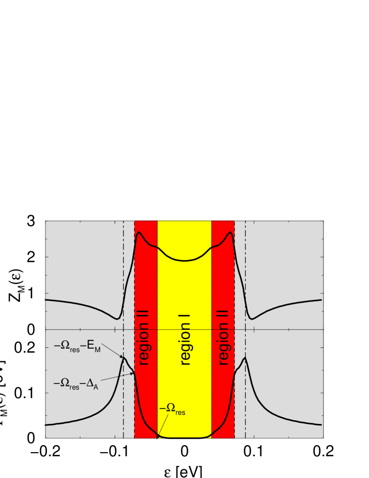
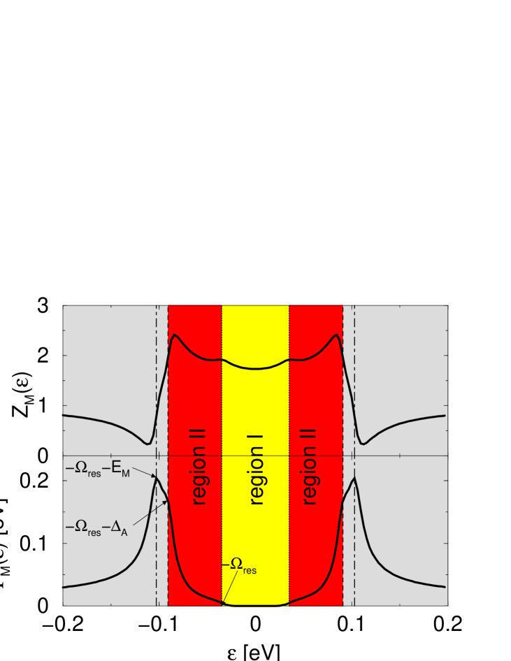
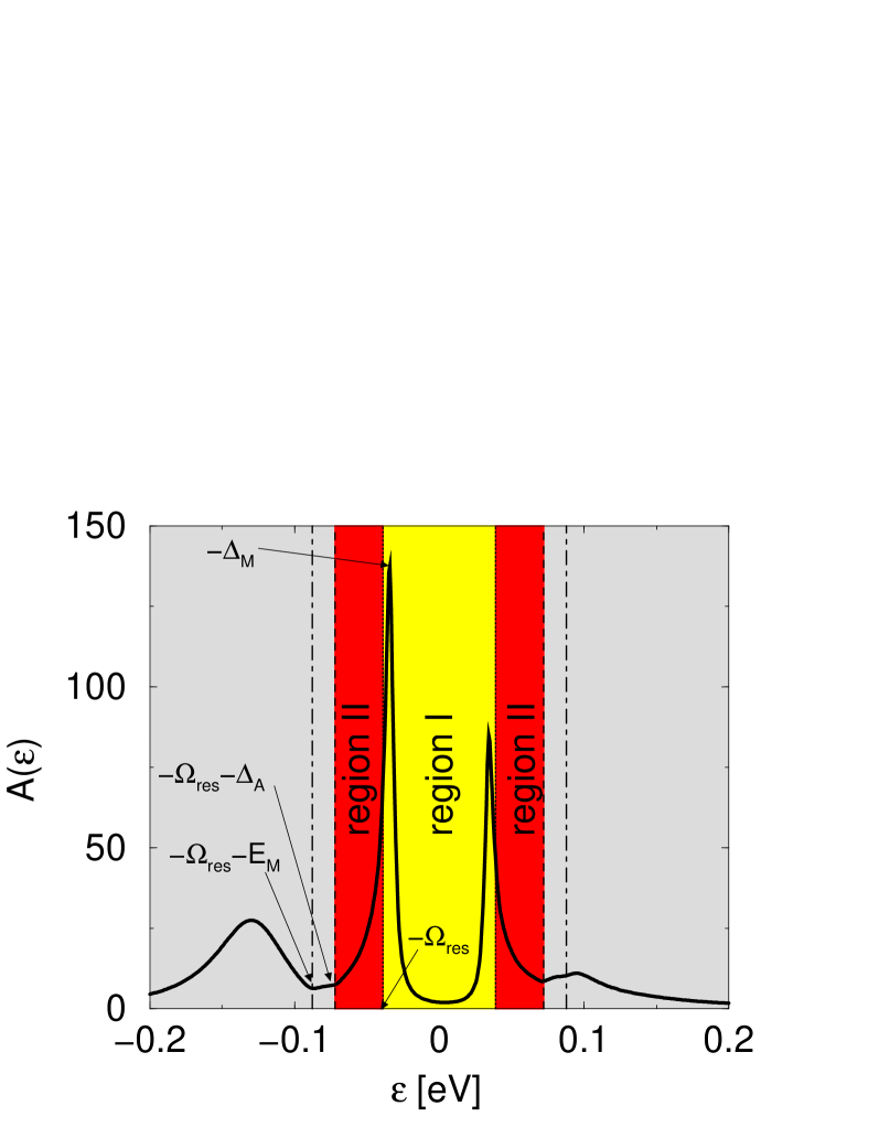
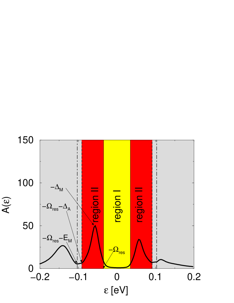
Figure 58: Spectral functions at $M$ for the self energies shown in the upper panels. The left two pictures are for optimally doped materials ($\Delta_{max}=35$meV, $\Omega_{res}=39$ meV) and the right two pictures for underdoped materials ($\Delta_{max}=60$ meV, $\Omega_{res}=35$ meV). A residual quasiparticle width of $\delta=5$ meV was assumed. (After Ref. [25], Copyright ©2003 APS).

The main features of the spectral function is the dip feature at an energy of about the resonance energy relative to the peak [15, 14, 16, 301, 17]. The peak position at $-\tilde{E}_{M}$ is renormalized by self-energy effects discussed above, and is shifted from the bare $-E_{M}$ to be near $-\Delta_{M}$. The dip feature is actually spread out over a range of size $E_{M}-\Delta_{A}$, and it is the onset of this dip feature which defines the resonance energy, $\Omega_{res}$. The dip feature is followed by a hump at higher binding energies, and the position of the hump maximum is very sensitive to the coupling constant and to damping due to the spin fluctuation continuum, as we show later. Thus, we concentrate in the following on the peak-dip structure. Another feature worth mentioning is the asymmetry of the lineshape at positive and negative binding energies, with a relatively weak dip feature on the unoccupied side compared to the occupied side.

The important difference between the left and the right pictures in Fig. refWwidth points out the role of the two regions, region I and II, for the spectral functions. In the left picture, the maximal gap $\Delta_{max}$ is less than the resonance frequency $\Omega_{res}$. Consequently, the quasiparticle peaks are situated in region I, slightly below the onset of damping due to scattering with the resonance mode. For overdoped materials it moves even further away from region II, becoming sharper, and the peak width is set in this case by the residual broadening due to other processes. In contrast, in the right picture of Fig. 58 the quasiparticle peak is situated in region II. Here, the maximal gap $\Delta_{max}$ is larger than the resonance frequency, and strong quasiparticle damping reduces the heights of the quasiparticle peaks. The width of the peak is given in this case by Eq. (105). For decreasing resonance mode energy, the peak weight is reduced and the incoherent part of the spectral function grows, taking weight from the quasiparticle peak. The hump energy is moving to higher binding energy with increasing coupling constant $g$ and increasing $\xi_{M}$. The weight of the peak is strongly reduced with increasing coupling constant. This is not the case with varying $\xi_{M}$.

The coherent weight of the quasiparticle peak, $z_{M}$, is only weakly dependent on the gap and the band structure in the relevant parameter range. It is proportional to the mode energy $\Omega_{res}$; together with the experimental finding $\Omega_{res}\propto k_{B}T_{c}$, this means $z_{M}\propto k_{B}T_{c}$. For coupling constants of order the band width or larger, $z_{M}\propto 1/(g^{2}w_{Q})$; for smaller coupling constants, $1/z_{M}\sim A+Bg^{2}w_{Q}$ with $A$ and $B$ constants. Finally, $z_{M}$ weakly decreases with increasing antiferromagnetic correlation length $\xi_{sfl}$.

We can understand some of these features using the approximate expression of Eq. (100). Evaluating $Z_{M}(\epsilon)$ at $\epsilon=-E_{M}$, and taking into account the coherence factor at the $M$ point, $A^{-}_{M}\equiv A^{-}_{M}(-E_{M})$, and the nodal renormalization factor $Z_{M}^{(N)}\equiv 1+\lambda_{M}^{(N)}(-E_{M})$, gives [25]

$$z_{M} \approx \frac{\Omega_{res}A^{-}_{M}}{Z_{M}^{(N)}\Omega_{res}+\frac{g^{2}I_{0}}{\pi(\Omega_{res}+2E_{M})}}$$ (107)

which defines the constants $A$ and $B$.

4.4 Contribution of the spin fluctuation continuum

For an understanding of the high-energy part of the electronic spectra and dispersions it is necessary to include also the continuum part of the spin fluctuation spectrum. The onset energy for the spin fluctuation spectrum determines the onset of strong scattering of electrons and the complete destruction of quasiparticle excitations. The spin fluctuation continuum extends to electronic energies ($\sim$ eV), and as a consequence the electronic scattering rate will increase continuously with energy up to electronic energies as well. In this section we discuss the implications of the additional scattering due to the spin fluctuation continuum in an extended model including the full model spectrum displayed in Fig. 54, and described by Eqs. (85) and (87). The low-energy gap of $2\Delta_{h}$ is determined by the superconducting gap at the ‘hot spot’ wavevectors as discussed in section 3.2. The momentum dependence of the continuum part of the spectrum is described well by Eq. (87), with a correlation length $\xi_{c}=0.5a$ compatible with experimental findings for near optimal doping. For this correlation length, the momentum average of $c_{q}$ gives $0.5c_{Q}$. Comparing with the experimental data for the momentum averaged susceptibility at 65 meV, which was found to be $6\mu_{B}^{2}/$eV for underdoped YBa₂Cu₃O_7-δ in the odd channel, and about $3\mu_{B}^{2}/$eV in the even channel [109], gives $c_{Q}\approx 6/$eV and $3/$eV respectively. The values for optimal doping should be smaller, and in Ref. [25] $c_{Q}=5.6/$eV and $g=0.65$ eV was found to reproduce well the experimental high energy (linear in excitation energy) part of the momentum linewidth in optimally doped Bi₂Sr₂CaCu₂O_8+δ, which gives $\Gamma_{N}=0.75\epsilon$ [179, 190]. This coupling includes both the even and odd (with respect to the bilayer indices) contributions of the spin fluctuations [93]. In contrast, the resonance mode is dominant in the odd channel, [81], and only recently there has been resolved a weaker resonance mode in the even channel as well [116, 92]. It is thus a good approximation to neglect the even channel contribution of the resonance mode and to only take into account the odd channel mode.

In this section we discuss first theoretical results without taking into account bilayer splitting. We will turn to the case of bilayer splitting in the next section.

The continuum eventually will be cut-off at electronic energies. However, the precise high-energy behavior of the spin fluctuation continuum is irrelevant, as it only leads to a contribution to the real part of the self energy that is almost energy independent (varying on the cut-off energy scale). This energy independent renormalization can be absorbed into a change of the bandwidth of the (bare) dispersion $\xi_{k}$ (and possibly of the ‘bare’ maximal $d$-wave gap $\Delta_{k}$). The corresponding renormalization factor $Z_{HE}$ has to be regarded as an additional phenomenological parameter. The experiments near optimal doping can be reproduced best by rescaling the dispersion from Table 4.2.1 in the following way:

$$\xi_{k}^{(new)}=Z_{HE}\xi_{k}-(Z_{HE}-1)\xi_{M}$$ (108)

with $Z_{HE}=1.5$ [25]. With this choice, the van Hove singularity at the $M$ point has the same distance from the chemical potential as before. The choice of parameters for the extended model additional to those in Table 4.3 is summarized in Table 4.4.

Additional parameters for the spin-fluctuation continuum used in the extended model of Ref. [25]. $2\Delta_{h}$ $\xi_{c}$ $\frac{1}{2}g^{2}c_{Q}$ $Z_{HE}$ 63 meV $0.5a$ 1.18 eV 1.5

The main results for the self energy effects are summarized for the $M$ point and the nodal point of the Brillouin zone in Figs. 59 and 60. The continuum contribution to the self-energy is shown as a dotted line, and the mode contribution as dashed line. As can be seen from the figures, the continuum contribution to the scattering rate sets in above the structures which are induced by the mode. It also contributes considerably to the renormalization of the low-energy dispersion, as the slope of the real part of the self energy shows. The high-energy region of the imaginary part of the self energy is drastically modified by the continuum contribution, and shows a region of linear in energy increase extending to rather high energies (the high-energy cut-off for the continuum spectrum in the calculations). In contrast, the mode contribution to the imaginary part of the self energy is in the high-energy region decaying with increasing energy. An interesting feature is that the mode contributes to the real part of the self energy a rather constant negative contribution. This feature will have interesting consequences when turning to the case of bilayer splitting (see next section), where this constant high-energy contribution to the real part of the self energy can differ for bonding and antibonding bands.

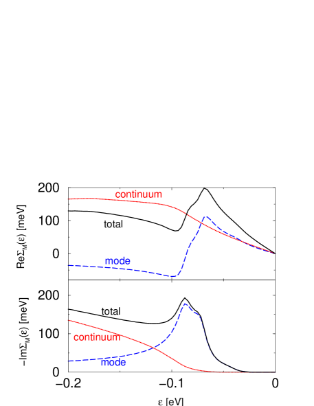
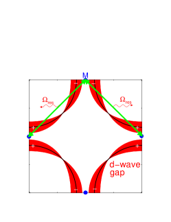
Figure 59: The different contributions to the real part (top) and the imaginary part (bottom) of the self energy are shown for the $M$ point. Dotted curves are the contribution from the spin fluctuation continuum, dashed the contribution from the spin fluctuation mode, and full both contributions. Calculations were done for the parameters of Tables 4.3 and 4.4, except $Z_{HE}=1$. The relevant scattering processes are shown on the right.

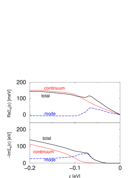
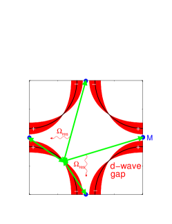
Figure 60: The different contributions to the real part (top) and the imaginary part (bottom) of the self energy are shown for the $N$ point. Dotted curves are the contribution from the spin fluctuation continuum, dashed the contribution from the spin fluctuation mode, and full both contributions. Calculations were done for the parameters of Tables 4.3 and 4.4, except $Z_{HE}=1$. The relevant scattering processes are shown on the right.

The self energy at the nodal point is very similar to the experimentally observed ones along the nodal direction [177, 34], apart from the low-energy scattering gap, which in experiment shows additional contributions that are not taken into account in the present theory. These additional contributions most probably stem from the incommensurate part of the spin-fluctuation spectrum, which couples most strongly to the nodal quasiparticles.

The difference in the relative magnitude between the mode contribution and the continuum contribution in Figs. 59 and 60 is explained in terms of different scattering geometries in the right panels of the figures. Because the mode is sharper in momentum than the continuum is, its contribution in the nodal case is reduced by the fact that the momentum vectors connecting the nodal points to the antinodal regions are far off the $(\pi,\pi)$ wavevector (see Fig. 60 right). Thus, the effect of the mode is reduced at the nodes, and in strongly overdoped materials in fact not observed in experiment (see Fig. 35) [36, 217]. It is however clearly observed as a kink in Im$\Sigma$ for underdoped and moderately overdoped materials, as seen from Fig. 39 [40]. This kink is consistent with the mode contribution in the theoretical results shown in Fig. 60, but not with the rather smooth onset of the continuum contribution only (dotted line).

Finally, note that for underdoped and optimally doped materials, where in the normal state the even channel stays gapped [82], the corresponding contribution of the even channel spin susceptibility to the normal state self energy is given by half the continuum contribution in Fig. 60. This will induce a weaker kink feature in the normal state at an energy equal to the even channel (optical) gap in the spin susceptibility, which is around 50-60 meV.

4.5 Renormalization of EDC and MDC dispersions

In this section theoretical results for the spectral functions and dispersion anomalies in a model using both the mode and the gapped continuum of the spin fluctuation spectrum are summarized. Results are shown for both EDC and MDC derived dispersions.

In Figs. 61-64, ARPES spectra and corresponding dispersions are shown along several selected paths in the Brillouin zone, indicated in the right panels of the figures. In the left panels of the figures, the intensities and spectral lineshapes can be followed, and in the middle panels, the corresponding dispersions of the peak maxima and hump maxima in the EDC’s are shown as circles, and the maxima in the corresponding MDC dispersions as curves. As can be seen from these figures, the linewidth of the spectral features are in general considerably broader in the high-energy region than in the low-energy region. This is in agreement with the experiments.

In Fig. 61 the cut is going from the $M$ point of the Brillouin zone toward the $Y$ point. The $A$ point (normal state Fermi crossing) corresponds to spectra roughly in the middle of the set.

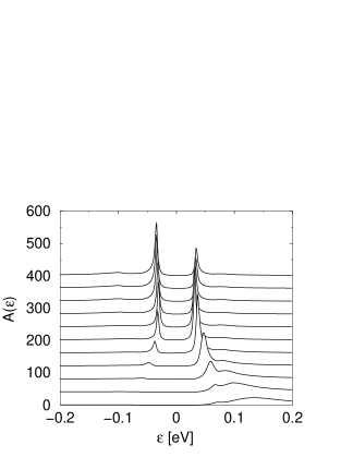
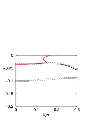
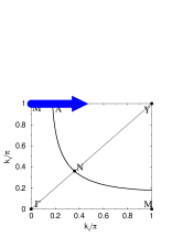
Figure 61: Left: Dispersion of the spectral intensity and lineshape as a function of momentum along the $M-Y$ cut, ($k_{y}=\pi$, $k_{x}=0...0.4\pi$ in steps of $0.04\pi$ from top to bottom). Middle: EDC (circles) and MDC (curve) dispersions from maxima of the curves shown in the left panel. In the EDC dispersion, the low energy peak and the high energy hump with the break feature in between is clearly visible. Because the bottom of the normal state dispersion is at $\xi_{M}=-34$meV, the MDC shows only a broad maximum at $M$ for high energies. (After Ref. [25], Copyright ©2003 APS).

Sharp quasiparticle excitations are present between the $M$ and $A$ points, and the dispersion (both EDC and MDC derived) is very flat, in agreement with the experimental findings of Ref. [34] (see Fig. 19 top panel). The MDC variation within the gap edge is observed experimentally (see section 2.2.7) and has been discussed in Ref. [30]. At high energies, the MDC is peaked at $M$.

Fig. 62 shows results along a cut in $M$-$\Gamma$ direction. The main features here are summarized as follows. There is an extremely flat behavior in the EDC hump-dispersion in the region between the $M$ point and roughly $0.3\pi$ from there in direction of $\Gamma$, and in this region the peak disperses only moderately. Quasiparticle peaks are observed in the entire region where the hump dispersion stays flat.

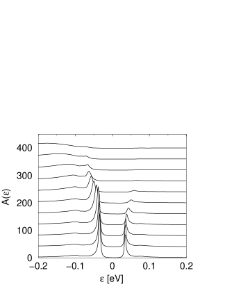
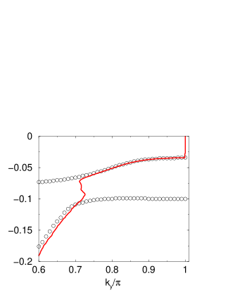
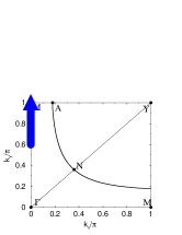
Figure 62: Left: Dispersion of the spectral intensity and lineshape as a function of momentum along the $M-\Gamma$ cut ($k_{x}=0$, $k_{y}=0.6\pi..\pi$ in steps of $0.04\pi$ from top to bottom). Middle: EDC (circles) and MDC (curve) dispersions from maxima of the curves shown in the left panel. (After Ref. [25], Copyright ©2003 APS).

The MDC shows an $S$-shaped behavior in the break region between the EDC peak and hump, and roughly at the point where the hump starts to disperse strongly away from the chemical potential. There is a weak maximum in the hump dispersion at $q_{y}\approx 0.85\pi$, that is due to the coupling of the $(\pi,0)$ and $(0,\pi)$ points by self-energy effects. This maximum corresponds to the Fermi crossing in the path displaced by $(\pi,\pi)$ from the one shown in the right panel of Fig. 62, and that corresponds to the one shown in the right panel of Fig. 63. This effect was observed experimentally [32], as shown in Fig. 20.

Fig. 63 shows the results for a cut parallel to the $M-Y$ between the antinodal and the nodal point, keeping $q_{y}=0.6\pi$ constant.

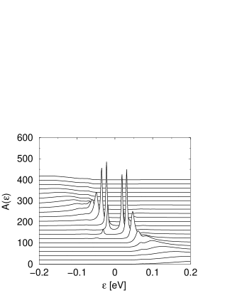
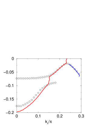
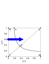
Figure 63: Left: Dispersion of the spectral intensity and lineshape as a function of momentum $k_{y}=0.6\pi$, $k_{x}=0...0.4\pi$ in steps of $0.02\pi$ from top to bottom. Middle: EDC (circles) and MDC (curve) dispersions from maxima of the curves shown in the left panel. (After Ref. [25], Copyright ©2003 APS).

This cut compares to the experimental findings in Fig. 19 and Fig. 21. At low energies, the spectral evolution, seen on the left part of the figure, shows the typical BCS mixing between particle and hole states. The EDC dispersions show a low-energy peak branch and a high-energy hump branch, separated by a dispersion break. The MDC shows in the break region an $S$-shaped dispersion anomaly. As was discussed in section 2.2.7, such $S$-shaped MDC derived dispersions correspond to important many-body renormalization effects in the superconducting state dispersion relative to that in the normal state and are observed experimentally. The MDC dispersion changes from the low energy peak branch to the high energy hump branch at roughly the point where the intensity of the peak drops dramatically. Note that the EDC and MDC dispersions are considerably displaced relative to one another at high energies. Also at low energies, the MDC dispersion is stronger near the break region than the EDC dispersion. This effect increases when the residual width of the quasiparticle peak increases, and when convolution with the experimental resolution function is taken into account [30].

It was mentioned in section 2.2.7 that the $S$-shaped dispersion in the MDC spectra is not observed experimentally in nodal direction, but is replaced by a kink-like feature. The fact, that an $S$-shaped dispersion is not observed in the nodal MDC spectra was shown to be inconsistent with an interpretation of the nodal self-energy effects in terms of electron-phonon coupling only [302]. In Fig. 64 we show the theoretical results for the cut along the nodal direction.

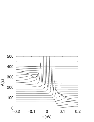
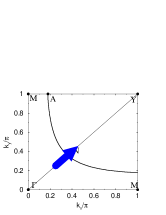
Figure 64: Left: Dispersion of the spectral intensity and lineshape in the nodal direction ($\Gamma-Y$) as a function of momentum $k_{x}=k_{y}=0.25\pi...0.45\pi$ in steps of $0.01\pi$ from top to bottom. Middle: the corresponding EDC (circles) and MDC (curve) dispersions. The kink is most clearly seen in the MDC dispersion. The low energy velocity is roughly half the high energy one. The high energy dispersion does not extrapolate to the Fermi surface crossing. (After Ref. [25], Copyright ©2003 APS).

Along the nodal direction the superconducting gap vanishes as a consequence of $d$ wave symmetry, and as a result there is a Fermi crossing of the dispersion. As can be seen in the left panel of Fig. 64, The dispersions kink in the MDC derived dispersion is observed in experiments along the nodal direction. It is reproduced rather well in the middle panel of Fig. 64. This is a result of the presence of the gapped continuum in addition to the sharp mode [25, 302]. Quasiparticle peaks are well defined only in the region below the kink energy, as seen clearly in the left panel of that figure. Note that the kink corresponds to the binding energy $\Omega_{res}+\Delta_{A}$, where $\Delta_{A}$ is the gap at the antinodal Fermi surface point. The damping sets in at binding energy $\Omega_{res}$, at slightly lower energies, due to the onset of node-node scattering processes, as can be seen in the left panel of Fig. 64. The velocity renormalization for low energies and high energies differs by a factor of roughly two, both for EDC’s and MDC’s, in agreement with experiment [34]. The high energy dispersion does not extrapolate to the Fermi crossing, again in agreement with experiments [33, 49]. Again, note some shift between the EDC and MDC dispersions at high energies due to the energy variation of the self energy.

Clearly, the velocity break (kink) along the nodal direction and the break between the peak and hump (dip) near the $M$ point are occurring in the same energy range between $-\Omega_{res}-\Delta_{A}$ and $-\Omega_{res}-E_{M}$ [7, 25]. This is an appealing result because it explains all features in the dispersion anomalies in the Brillouin zone seen by ARPES within the same model.

4.6 Bilayer splitting

ARPES experiments on bilayer cuprate superconductors have been able to resolve a bilayer splitting between bonding and antibonding bands [188, 35, 146, 173]. The dispersion near the $(\pi,0)$ point of the Brillouin zone shows an unusual asymmetry between bonding and antibonding self-energy effects. In particular, Feng et al. [188] found that the EDC-derived dispersions in overdoped Bi₂Sr₂CaCu₂O_8+δ ($T_{c}=65$K) consist of three features: an antibonding band (AB) peak near 20 meV, a bonding band (BB) peak near 40 meV, and a bonding hump near 105 meV. Gromko et al. [178, 36] reported strong self-energy effects in the dispersions derived from MDC’s in similar samples ($T_{c}=58$K). Near momentum $(k_{x},k_{y})=(1,0.13)\pi/a$, an $S$-shaped dispersion anomaly, discussed previously in Ref. [30], was shown to be present only in the bonding band MDC, at binding energies between 40 meV and 60 meV. In both experiments, a low energy double peak structure in the EDC was only resolvable in the same momentum region. In recent experiments by Borisenko et al. [193, 170] it was found that the asymmetry between bonding and antibonding self-energy effects leads to a different behavior in the imaginary part of the self energy as a function of binding energy. This behavior was previously predicted in Ref. [24], where it was shown to be a result of the odd parity of the resonance mode with respect to the exchange of the bilayer indices. It is argued there, that low energy scattering of electrons between the bonding and antibonding bands is strong compared to scattering within each of those bands. As scattering events which connect different bilayer bands are odd with respect to permutation of the layers within a bilayer, this implies that the corresponding bosonic excitations which mediate such scattering must be dominant in the odd channel. The model explains all of the above cited experimental features, and the very recent experiments [193, 170] give strong additional support for the model.

For electrons phase coherent between the two planes of a bilayer, the spectra will exhibit separate bonding ($b$) and antibonding ($a$) features with (normal state) dispersions given by Eq. (77). In the superconducting state, the dispersions are modified by the presence of the $d$-wave order parameter Eq. (75). In agreement with experiment [188, 146, 173], $\Delta_{M}$ is assumed to be the same for the bonding and antibonding bands. Then, the BCS dispersion in the superconducting state takes the form

$$E^{(a,b)}_{{\bf k}}=\sqrt{(\xi^{(a,b)}_{{\bf k}})^{2}+(\Delta_{{\bf k}})^{2}}.$$ (109)

It is clear that the observed dispersion features are many-body effects beyond Eq. (109). In the following we review the theoretical results from Ref. [24] and compare them directly with the experimental results. The employed model includes coupling of electrons to the resonant spin-1 mode as well as a gapped spin fluctuation continuum. From section 2.1.3 the spin susceptibility in bilayer materials is a matrix in the layer indices, having elements diagonal ($\chi_{aa}$, $\chi_{bb}$) and off-diagonal $(\chi_{ba}$, $\chi_{ab}$) in the bonding-antibonding representation. The resonance part, $\chi_{res}$, was experimentally found to be dominated by the odd channel, whereas the continuum part, $\chi_{c}$, enters in both [93]. Assuming that the intensity of the even resonance is negligible, (its intensity is so small that it was found only recently), the corresponding even and odd susceptibilities are,

$$\chi_{o}(\Omega,{\bf q}) = \chi_{res}(\Omega,{\bf q})+\chi_{c}(\Omega,{\bf q}),$$ (110)

$$\chi_{e}(\Omega,{\bf q}) = \chi_{c}(\Omega,{\bf q}).$$ (111)

This means that the resonance mode can only scatter electrons between the bonding and antibonding bands. In contrast, the spin fluctuation continuum scatters both within and between these bands. As argued in Ref. [24], the odd symmetry of the resonance is crucial in reproducing the ARPES spectra.

Writing the self energy symbolically as $\hat{\Sigma}=g^{2}\chi\ast\hat{G}$ (the hat denotes the 2x2 particle-hole space, and $g$ is the coupling constant), the self energy $\hat{\Sigma}^{(a,b)}$ for the antibonding and bonding bands are given as [24],

$$\hat{\Sigma}^{(a,b)}=\frac{g^{2}}{2}\left\{\chi_{res}\ast\hat{G}^{(b,a)}+\chi_{c}\ast\left(\hat{G}^{(b)}+\hat{G}^{(a)}\right)\right\}.$$ (112)

Dispersion anomalies arise mainly from coupling to the resonance mode. This means that dispersion anomalies in the bonding band are determined by the antibonding spectral function and vice versa. Because the antibonding band is (in contrast to the bonding band) close to the chemical potential at $(\pi,0)$ [188], the associated van Hove singularity leads to a larger self energy for the bonding band.

The spin-fluctuation spectrum is modeled by Eqs. (83)-(85). Parameters are chosen appropriate for the overdoped sample ($T_{c}=65$K) studied in experiment [163, 167]. The normal state dispersion is obtained from a 6 parameter tight-binding fit to experimental data [303], plus the bilayer splitting discussed earlier. The seven parameters used for this fit are obtained from the second line in Table 4.2.1. The high energy ($|\epsilon|{{}_{\textstyle>}\atop{\textstyle\sim}}200$ meV) dispersions are not affected strongly when going from the normal to the superconducting state. However, even in the normal state, the bare dispersion is renormalized by the normal state spin fluctuation continuum. The extra factor $Z_{HE}=1.4$ in Eq. (108) accounts for this extra renormalization. For the remaining parameters of the model, the values shown in Table 4.6 were used.

Minimal parameter set used in the calculations for an overdoped bilayer material [24]. $\Delta_{M}$ $\Omega_{res}$ $\xi_{M}^{(a)}/\xi_{M}^{(b)}$ $\xi_{sfl}$ $g^{2}w_{Q}$ $2\Delta_{h}$ $\xi_{c}$ $g^{2}c_{Q}$ $Z_{HE}$ 16 meV 27 meV $-18/-105$ meV $2a$ 0.15 eV² 28.8 meV $0.5a$ 0.72 eV 1.4

The value for the resonance energy was obtained from the relation $\Omega_{res}=4.9k_{B}T_{c}$ found experimentally to hold for overdoped Bi₂Sr₂CaCu₂O_8+δ [94, 99, 44]. With the parameters of Table 4.6 the resonance weight is $0.36\mu_{B}^{2}$ per plane, and the (2D)-momentum averaged continuum contribution (gotten by summing the even and odd channels for energies $\omega{{}_{\textstyle<}\atop{\textstyle\sim}}0.2eV$) amounts to $1.7\mu_{B}^{2}/$eV per plane.

The bonding and antibonding normal state Fermi surfaces are shown in Fig. 65 a.

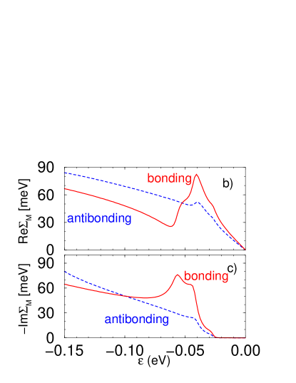
Figure 65: (a) Tight binding Fermi surfaces for antibonding and bonding bands in overdoped Bi₂Sr₂CaCu₂O_8+δ ($T_{c}=65$K). (b) Real part and c) imaginary part of the self energy at the $(\pi,0)$ point of the zone for the bonding band (BB) and antibonding band (AB). (After Ref. [24], Copyright ©2002 APS).

The bilayer splitting is maximal near the $(\pi,0)$ points of the zone. In Fig. 65 b the real part of the self energy for bonding and antibonding bands at the $(\pi,0)$ point is shown. The renormalization effects are stronger for the bonding band than for the antibonding band. This is a result of the proximity of the antibonding saddle point singularity to the chemical potential. As is seen in this figure as well, both bands are renormalized up to high energies. Note the linear in binding energy high-energy contribution in Re $\Sigma$. It has the same slope for bonding and and antibonding self energy, however there is a shift with respect to each other. The constant shift is the consequence of the mode contribution, whereas the term linear in binding energy comes from the continuum part of the spin fluctuation spectrum. As the continuum contribution is the same in even and odd channels, the high-energy slope of Re $\Sigma$ in Fig.65 is identical.

The imaginary part of the self energy is shown in Fig. 65 c) for the bonding and antibonding bands. As emission processes are forbidden for $|\epsilon|<\Omega_{res}$, the imaginary part of the self energy is zero in this range. Due to scattering events to the antibonding band, electrons in the bonding band have a large imaginary part of the self energy in the range between 40 and 60 meV. These events are dominated by emission of the resonance, and are enhanced due to the van Hove singularity in the antibonding band close to the chemical potential. In contrast, the imaginary part of the antibonding self energy is not enhanced because the bonding band is far from the chemical potential at $(\pi,0)$. Consequently, it shows linear behavior over a wide energy range, with a gap at low energies ($|\epsilon|<\Omega_{res}$).

In Fig. 66 we compare theoretical calculations of the model in Ref. [24] with the experimental results of Ref. [193].

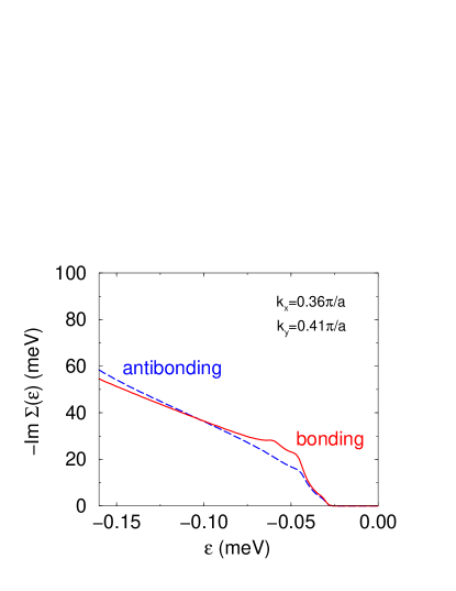
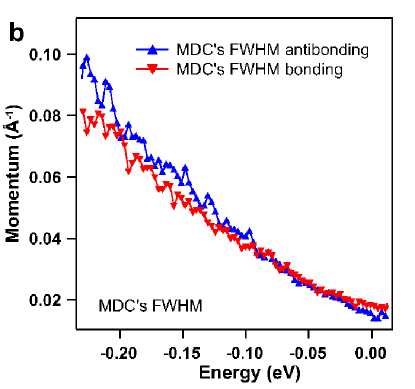
Figure 66: Left: Imaginary part of the self energy, calculated within the model in Ref. [24], at the ${\bf k}$-point $(0.36,0.41)\pi/a$, which is situated at the Fermi surface close to the nodal point $(0.37,0.37)\pi/a$ of the order parameter. Calculations are done for the bonding band (BB) and antibonding band (AB). Right: Experimental data from Ref. [193], showing the MDC full width half maximum for a (Pb,Bi)₂Sr₂CaCu₂O_8+δ sample as a function of energy, separately for the bonding and antibonding band, at a ${\bf k}$-vector close to the node of the order parameter. The MDC-widths are proportional to the imaginary part of the self energy. (From Ref. [193], Copyright ©2006 APS).

The behavior of the imaginary part of the self energy, here shown closer to the nodal point, is qualitatively similar to that of Fig. 65 c). At low energies the bonding band damping is stronger than the antibonding band damping. At higher binding energies these roles are switched. The crossover takes place at binding energy of about 100 meV. This is completely in agreement with the experiment.

Fig. 67 presents the ARPES intensities for the bonding and antibonding spectra and compare with the experimental spectra fro Ref. [163]. The antibonding spectra consist of a low energy AB peak, and the bonding

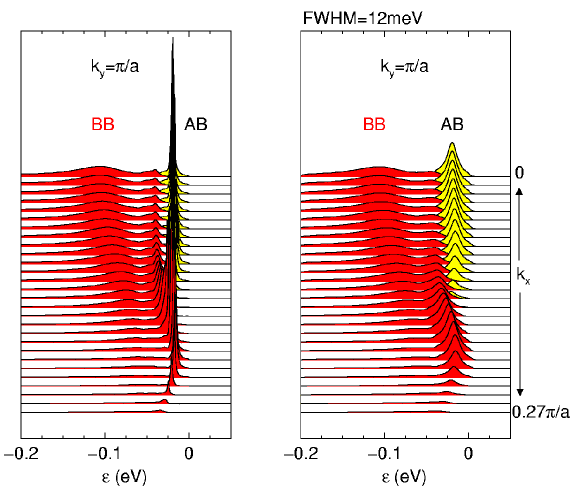
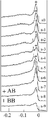
Figure 67: The left two panels show the calculated ARPES intensity appropriate for overdoped ($T_{c}=65$K) Bi₂Sr₂CaCu₂O_8+δ, for $k_{y}=\pi/a$, and $k_{x}$ varying from $0$ to $0.27\pi/a$, at $T=10$K. For comparison with experiment, in the middle the spectra convolved with a Lorentzian energy resolution function (FWHM 12 meV) are shown (after Ref. [24], Copyright ©2002 APS). On the right experimental data from Ref. [163] are shown for comparison. The spectrum s0 corresponds to $k_{x}=0$, and the spectrum s9 to $k_{x}=0.24\pi/a$. The crosses and bars denote the antibonding and bonding peaks, respectively. (From Ref. [163], Copyright ©2001 APS).

spectra have a low energy BB peak and a higher energy BB hump feature. In agreement with experiment ([163] and [178]), the width of the EDC spectrum is large for the BB hump, but not so for the BB and AB peaks. As can be seen from Fig. 67 (left), the BB peak is well defined even near $(\pi,0)$, however the finite energy resolution, (taken into account in middle of Fig. 67) renders it unobservable in experiment.

In Fig. 68 results for the dispersion of the EDC peak positions are shown and compared with the experimental dispersions of Ref. [163].

             

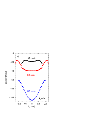
Figure 68: Left: Calculated dispersion of EDC peak positions (appropriate for overdoped $Bi_{2}Sr_{2}CaCu_{2}O_{8+\delta}$ with $T_{c}=$65 K) near the $(\pi,0)$ point of the Brillouin zone (after Ref. [24], Copyright ©2002 APS). The EDC dispersion consists of three branches, one antibonding peak, one bonding peak and one bonding hump. Right: Experimental dispersion of the superconducting peaks for the bonding (bars) and antibonding (crosses) band, compared to the normal state bonding (solid circles) and antibonding (triangles) bands for an overdoped $Bi_{2}Sr_{2}CaCu_{2}O_{8+\delta}$ sample width $T_{c}=$65 K (from Ref. [163], Copyright ©2001 APS).

The experimentally observed three branches [163, 178] are reproduced, one antibonding peak and two bonding branches, denoted ‘BB peak’ and ‘BB hump’. The BB peak has a very flat dispersion near $k_{x}=0$ in agreement with experiment [163], as shown in the right picture in Fig. 68. The position of that BB peak at 40 meV is approximately given by $\Omega_{res}+\Delta_{A}$, where $\Delta_{A}$ is the gap at the antibonding Fermi crossing. Thus, the energy separation between the AB peak at the AB Fermi crossing and the BB peak at $(\pi,0)$ is a measure of the resonance mode energy $\Omega_{res}$ in overdoped compounds. The BB hump position at high binding energies (105meV) is determined by the normal state dispersion of the bonding band. Because the spin fluctuation continuum changes only at low energies when going from the normal to the superconducting state, the position of the BB hump maximum is not very different from the normal state BB dispersion. This is in agreement with experiment [163]. The intensity of the AB peak decreases quickly when it approaches the BB peak, but is strong at $(\pi,0)$ because of the proximity of the AB band to the chemical potential in this region.

In Fig. 69, the theoretical results for the MDC dispersions are shown on the left side (for comparison also the EDC dispersions is shown as small symbols), and compared with the experimental ones of Ref. [178] (shown on the right side).

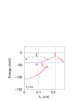
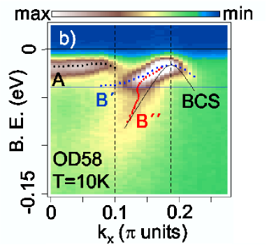
Figure 69: Left: Calculated dispersion of MDC peak positions (full symbols) (appropriate for overdoped $Bi_{2}Sr_{2}CaCu_{2}O_{8+\delta}$ with $T_{c}=$65 K) near the $(\pi,0)$ point of the Brillouin zone. The MDC bonding dispersion shows a characteristic $S$ shape behavior. The open symbols show again the EDC peak positions from Fig. 68 for convenience. (From Ref. [24], Copyright ©2002 APS). Right: Experimental superconducting state ARPES data for an overdoped ($T_{c}=$58 K) Bi₂Sr₂CaCu₂O_8+δ sample near the point $(\pi,0)$. (From Ref. [178], Copyright ©2002 UC). In both pictures, $A$ refers to the antibonding band peak positions, $B^{\prime}$ to the bonding band EDC peak position, and $B^{\prime\prime}$ to the bonding band MDC peak positions.

The MDC dispersion consists of two branches, an AB MDC branch and a BB MDC branch. The self-energy effects are most clearly observable in the BB MDC branch. In the binding energy range between 40meV and 60meV, there is an $S$-shaped ‘break’ region, connecting the BB hump EDC branch with the BB peak EDC branch. This $S$-shaped behavior reproduces the finding of the experiments [178].

Finally, in Fig. 70 spectra are shown for three positions in the Brillouin

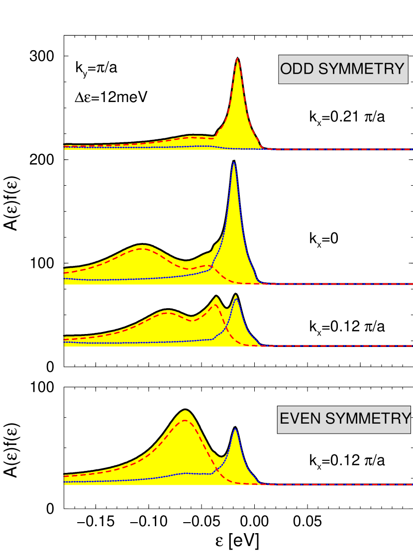
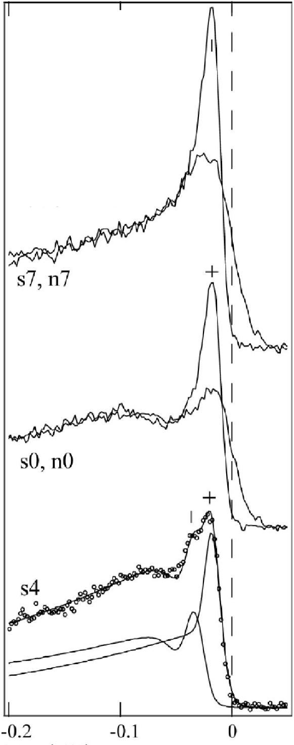
Figure 70: Left: Calculated ARPES intensities, appropriate for overdoped ($T_{c}=65$K) Bi₂Sr₂CaCu₂O_8+δ, for $k_{y}=\pi/a$ at $k_{x}=0$, $k_{x}=0.12\pi/a$ and $k_{x}=0.21\pi/a$. The full lines are the sum of antibonding (dotted) and bonding (dashed) spectral functions. Calculations are done for $T=10$K. For comparison with experiment, a Lorentzian energy resolution function of 12 meV width was assumed. The low energy double peak structure is clearly resolved for $k_{x}=0.12\pi/a$, as in experiment [163, 178]. It is not present if the mode is in the even channel, as demonstrated in the bottom panel. (After Ref. [24], Copyright ©2002 APS). Right: For comparison are shown experimental data for an overdoped ($T_{c}=65$K) Bi₂Sr₂CaCu₂O_8+δ sample at $T=10$K from Ref. [163] (Copyright ©2002 APS). The spectral functions s7, s0, and s4 should be compared with the upper three spectral functions in the left panel (the curves n0 and n7, having a broader peak than s0 and s7, are for the normal state).

zone, corresponding to the experimental spectra shown on the right side [163]. For each spectrum, the bonding (dashed) and antibonding (dotted) contributions are indicated. The spectra are convolved with a Lorentzian energy resolution function to allow for direct comparison with experiment. We reproduce all experimental findings. First, at $(\pi,0)$, only the BB hump and the AB peak are resolved. This is due to resolution effects mentioned above. Second, near the AB Fermi crossing, the spectra show a characteristic double peak structure, with a relatively sharp AB peak and a BB peak separated from a broad BB hump. Third, at the BB Fermi crossing, only the BB peak is observed. The BB hump is so small in intensity that it only leads to a kink-like feature in the spectrum.

The dispersion anomalies observed in the bonding band are a mirror of the large number of states close to the chemical potential near $(\pi,0)$ for the antibonding band. Scattering events involving a mode with energy $\Omega_{res}$ couple the bonding band electrons in the energy region between 40 and 60 meV strongly to those antibonding band electrons. The corresponding processes are in the odd channel. These effects would be lost if the resonance were in the even channel. In this case, the a,b indices in the first part of Eq. (112) would be reversed, and thus the assignments listed in Fig. 65 b and c. The antibonding van Hove singularity would no longer enter in the bonding self-energy. The consequence of this can be seen in the bottom panel of Fig. 70, where our calculations were repeated assuming an even symmetry mode. Only two spectral features occur now, not three. Moreover, the resulting MDC dispersion for the bonding band loses the anomalous $S$-shaped region seen in Fig. 68b.

As can be seen from Figs. 65-70 the agreement of the theory [24] with the experimentally observed self-energy effects in the bilayer split bands in bilayer high-temperature superconductors is very good. The theory reproduces quantitatively the EDC dispersions, the MDC dispersions, the spectral lineshapes, and the MDC widths. Calculations using a more sophisticated spin-fluctuation spectrum, obtained from a bilayer $t-t^{\prime}-J$ model, have confirmed this picture [304]. In conclusion, the ARPES data are consistent with the interaction of the electrons with a sharp bosonic mode which is predominantly odd in the layer indices, a property unique to the magnetic resonance observed by inelastic neutron scattering.

4.7 Tunneling spectra

Theoretical treatments for the connection between the dip-features in tunneling spectra and the magnetic resonance mode have been presented in Refs. [7], [18], [305] and [213]. In principle it is straightforward to calculate the tunneling density of states once the spectral function, $A(\epsilon,{\bf k})$, throughout the zone is known. The only complication arises from the tunneling matrix element $T_{{\bf k}{\bf p}}$, which can be very anisotropic in high-$T_{c}$ cuprates [166, 165].

The dip-hump structure, which is observed experimentally both in SIN and SIS junctions, was discussed by Eschrig and Norman [7] and by Abanov and Chubukov [18]. The processes, which lead to the dip in the density of states spectrum, are schematically sketched in Fig. 71.

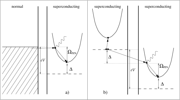
Figure 71: Schematic diagrams showing the processes responsible for the dip features in SIN (a) and SIS (b) tunnel junctions. For SIN tunneling, the electron that tunnels into the superconductor can emit a resonant spin wave with frequency $\Omega_{res}$ if the voltage $eV=\Delta+\Omega_{res}$. The electron is left at the bottom of the band, which leads to a sharp reduction of the current, leading to a drop in d$I/$d$V$. For SIS tunneling an electron pair must be broken first, which requires an energy $2\Delta$. In this case the dip in d$I/$d$V$ occurs at $eV=2\Delta+\Omega_{res}$. (From Ref. [306], Copyright ©2000 APS).

As can be seen, both for SIN and for SIS junctions the dip is produced at distance $\Omega_{res}$ from the coherence peaks, which are at $\Delta$ and $2\Delta$ respectively.

In the following we present numerical results from Ref. [7] which are calculated neglecting for simplicity the continuum part of the spin fluctuation spectrum. The numerical results for SIN and SIS junctions are shown in Fig. 72.

From the SIN tunneling current $I(V)$,

$$I(V)=\sum_{{\bf k}}|M_{{\bf k}}|^{2}\int_{-\infty}^{\infty}\frac{d\epsilon}{2\pi}A(\epsilon,{\bf k})\left\{f(\epsilon)-f(\epsilon+eV)\right\}$$ (113)

one obtains the differential conductance, $dI/dV$. Here, $M_{{\bf k}}$ is the SIN matrix element, assumed to be energy independent. The tunneling matrix element can be modelled for two extreme cases: for incoherent tunneling $|M_{{\bf k}}|^{2}=M_{0}^{2}$, whereas for coherent tunneling $|M_{{\bf k}}|^{2}=\frac{1}{4}M_{1}^{2}(\cos k_{x}-\cos k_{y})^{2}$ [166]. Coherent tunneling arises from hopping in c-axis direction via a complicated path of intermediate orbitals. The main contribution to the anisotropy comes from overlap between the Cu-$d_{x^{2}-y^{2}}$/O-$p_{x,y}$ hybrid orbitals with the O-$p_{z}$ orbitals. Coherent tunneling in the c-axis direction is strongly enhanced for the $M$ points in the Brillouin zone compared to the regions near the zone diagonal due to the matrix elements [166]. On the other hand, incoherent tunneling is via inhomogeneities or impurities that destroy the in-plane momentum conservation during tunneling events.

Results of such a calculation are shown in the top panels of Fig. 72.

Figure 72: Differential tunneling conductance for SIN (top) and SIS (bottom) tunnel junctions for $T=40$ K. Units are $eM_{i}^{2}$ for SIN and $2e^{2}T_{i}^{2}$ for SIS. Results for the incoherent (left) and coherent (right) tunneling limits are shown. Curves are for $g$=0.39 eV (dotted), 0.65 eV (full line), and 0.90 eV (dashed). The other parameters are given in Table 4.3. (From Ref. [7], Copyright ©2000 APS).

The low energy behavior of the tunneling spectrum in the coherent tunneling limit does not show the characteristic linear in energy behavior for $d$-wave, because the nodal electrons have suppressed tunneling as a result of the matrix elements. The peak-dip-hump features, on the other hand, are not affected by the matrix elements, as they are dominated by the $M$ point regions which are probed by both coherent and incoherent tunneling. The dip position stays roughly at the distance $\Omega_{res}$ from the peak position, whereas the higher energy features depend strongly on the coupling constant. Note the strong asymmetry of the dip-effect with respect to the chemical potential. The self energy effects are much stronger on the negative side than on the positive side of the spectrum, as in experiments [207, 208].

For an SIS junction, the single particle tunneling current is given in terms of the spectral functions by

$$I(V)=2e\sum_{{\bf k}{\bf p}}|T_{{\bf k}{\bf p}}|^{2}\int_{-\infty}^{\infty}\frac{d\epsilon}{2\pi}A(\epsilon,{\bf k})A(\epsilon+eV,{\bf p})\left[f(\epsilon)-f(\epsilon+eV)\right]\quad$$ (114)

with $|T_{{\bf k}{\bf p}}|^{2}=T_{0}^{2}$ for incoherent tunneling and $|T_{{\bf k}{\bf p}}|^{2}=\frac{1}{16}T_{1}^{2}(\cos k_{x}-\cos k_{y})^{4}\delta_{{\bf k}_{||},{\bf p}_{||}}$ for coherent tunneling [166]. Results for d$I$/d$V$ from Ref. [7] are shown in the bottom panels of Fig. 72. All structures are symmetric around the chemical potential. Again, the low energy part of the spectrum is strongly suppressed in the incoherent tunneling limit. At higher voltages, in the coherent tunneling limit, a negative differential conductance was predicted [7]. Such an effect has been observed in optimally doped Bi₂Sr₂CaCu₂O_8-δ break junctions [44]. The negative behavior at higher bias in the (purely) coherent tunneling limit was explained in Ref. [25], where it was pointed out that the continuum contribution will lead to a positive response at high voltages.

The difference between the incoherent tunneling limit and the coherent tunneling limit can be most clearly seen by the fact that at zero temperature the incoherent limit the SIS current is given by,

$$I^{(incoh)}(V)=\frac{eT_{0}^{2}}{\pi}\int_{-eV}^{0}d\epsilon N(\epsilon)N(\epsilon+eV),$$ (115)

whereas in the coherent limit it can be approximated by [25],

$$I^{(coh)}(V)\approx\frac{eT_{1}^{2}}{\pi}\int_{-eV}^{0}d\epsilon A_{M}(\epsilon)A_{M}(\epsilon+eV)$$ (116)

with $T_{1}^{2}=\sum_{{\bf k}{\bf p}}|T_{{\bf k}{\bf p}}|^{2}$. This latter expression results from the fact that tunneling is very effectively suppressed in the nodal direction for coherent tunneling, and mostly the $M$ point regions of the Brillouin zone are tested then. As a consequence, in the coherent limit tunneling tests the spectral function at the $M$ point of the Brillouin zone [25].

Spectra obtained from scanning tunneling spectroscopy (STS) were analyzed within the model of Eschrig and Norman [24] by Hoogenboom et al. [305]. They found that the tunneling data are reproduced only if interaction of quasiparticles with the collective mode is taken into account. A simple $d$-wave BCS model as well as a marginal Fermi liquid model fail to reproduce the tunneling data for reasonable parameters.

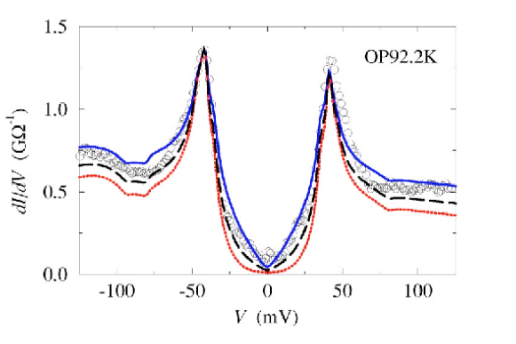
Figure 73: Comparison of STS spectra including the coupling the the resonance mode for coherent tunneling limit (dotted line), incoherent tunneling limit (full line) and a partially coherent tunneling with $|T_{{\bf k}}|^{2}=0.4|T_{inc}|^{2}+0.6|T_{coh}|^{2}$ (dashed line). Parameters are $\Delta_{M}=39$ meV, $g=0.65$ eV, $\xi_{sfl}=2a$, and $\Omega_{res}=5.4k_{\rm B}T_{c}$. (From Ref. [305], Copyright ©2003 APS).

In Fig. 73 the comparison of experimental data from optimally doped Bi₂Sr₂CaCu₂O_8+δ with the calculations of Ref. [305] is reproduced, showing that the data are best accounted for by assuming some partially coherent tunneling mechanism.

4.8 Doping dependence

In this section, we deal with the doping dependence of the spectral lineshape near the $M$ point of the Brillouin zone. It was shown in Ref. [25] that there are several general statements one can draw from the theoretical calculations of the electronic spectra resulting from an assumed coupling to the spin-1 magnetic resonance mode.

First, the relevant parameter which determines the behavior of the spectral functions and separates the underdoped region from the overdoped region is the parameter $\Omega_{res}/\Delta_{M}$. This parameter is roughly 1 for optimal doping, larger than 1 in the overdoped region and smaller than 1 in the underdoped region. It means that in the overdoped region the magnetic resonance is closer to the spin-fluctuation continuum and in the underdoped region closer to zero energy, the separation at optimal doping being roughly there where the resonance is halfway between zero energy and the energy of the continuum onset.

Second, the quasiparticle weight decreases with decreasing $\Omega_{res}/\Delta_{M}$ (as it does with increasing coupling constant $g^{2}w_{Q}$). Third, the quasiparticle scattering rate increases with decreasing $\Omega_{res}/\Delta_{M}$. And fourth, the hump energy disperses to higher binding energies for increasing coupling constant and increasing $\xi_{M}$. Thus, the theoretical predictions for electrons coupled to the spin-1 resonance mode in cuprates when going from overdoping to underdoping are a decreasing quasiparticle weight, an increasing quasiparticle scattering rate, and an increasing hump binding energy.

The situation is schematically shown in the phase diagram in Fig. 74. The curves shown are calculated using the formulas $T_{c}=95\mbox{ K}\left(1-82.6(p-0.16)^{2}\right)$ [307] and $\Omega_{res}=4.9T_{c}$ [44], where $p$ is the hole doping level in the Cu-O₂ planes. Optimal doping corresponds to $p=0.16$. The $\Delta_{M}$ variation is based on ARPES data [32, 123], and was modelled by $\Delta_{M}=38\mbox{ meV}\left(1-9.1(p-0.16)\right)$. All these quantities approach zero on the overdoped side at $p=0.27$.

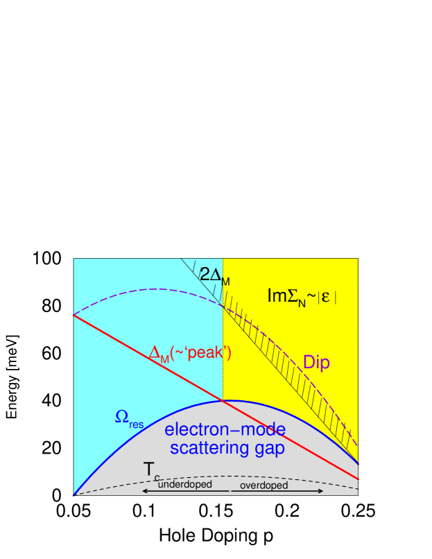
Figure 74: ‘Energy phase diagram’ for the coupling between electrons and the resonant spin-1 mode in the superconducting state. The resonance energy, shown as a thick line, is bounded from above by twice the maximal gap energy, $\Omega_{res}<2\Delta_{M}$, and approaches it on the overdoped side. The (antibonding for bilayer cuprates) peak position corresponds roughly to the value of $\Delta_{M}$. In the region below $\Omega_{res}$ no scattering between electrons and the resonance mode is possible. Quasiparticle peaks in this region are sharp. Above this line, strong damping sets in and the peak weight is strongly reduced on account of an incoherent high-energy background. The position of optimal doping, at maximal $T_{c}$ and $\Omega_{res}$, roughly coincides with the point where $\Delta_{M}$ as a function of doping crosses $\Omega_{res}$. In the overdoped region (toward the right) quasiparticles are well defined in the antinodal Fermi surface regions. With underdoping (toward the left) quasiparticles in the antinodal Fermi surface regions are progressively destroyed. (After Ref. [25], Copyright ©2003 APS).

The separation between overdoped and underdoped regions roughly coincides with the regions where $\Omega_{res}>\Delta_{M}$ and $\Omega_{res}<\Delta_{M}$, respectively. The dip onset is given by $\Omega_{res}+\Delta_{A}$, where $\Delta_{A}$ is the gap at the antinodal point of the Fermi surface. As $\Delta_{A}$ is about the same as $\Delta_{M}$, the line for $\Omega_{res}+\Delta_{M}$ shown as dashed line in Fig. 74 determines the position of the dip fairly accurately. The continuum in the spin fluctuation spectrum is gapped by $2\Delta_{h}$, and consequently only affects electrons above $2\Delta_{h}$, which is near or above the dip energy. This is the region in which a variation of the MDC widths linear in the binding energy can be observed (the magnitude of this linear term drops however towards overdoping, and a quadratic behavior was suggested in Ref. [40] to take over). The point of optimal doping for a Cu-O₂ plane roughly corresponds to the point where $\Omega_{res}/\Delta_{M}=1$. Another experimental observation is that this ratio never exceeds the value two. This is expected for an excitonic collective mode below a continuum edge [44].

The main feature is the ‘electron-mode scattering gap’ shown in Fig. 74 below $\Omega_{res}$. As $\Delta_{M}$ as a function of doping enters this gapped region at the overdoped side, all quasiparticle excitations along the Fermi surface (and also in the $M$ point regions) are well defined, showing up as rather sharp peaks. On the other hand, in the underdoped region, quasiparticles with binding energy $\sim\Delta_{M}$ is strongly scattered by the spin-1 resonance mode and are progressively destroyed toward underdoping. At the same time the weight of the quasiparticle peak is reduced on the account of an incoherent high-energy background above the dip energy.

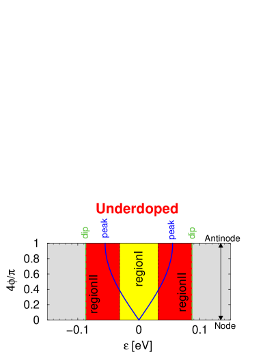
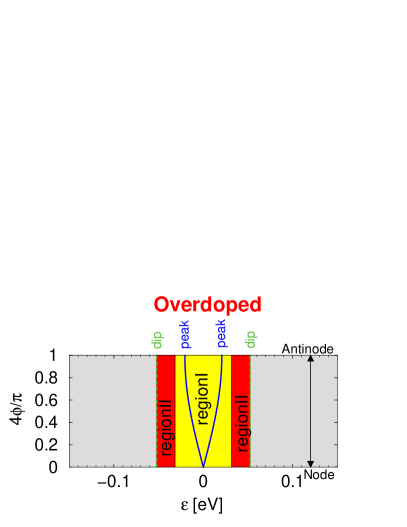
Figure 75: The full curves determine for each Fermi surface angle $\phi$ (which denotes the position along the Fermi surface and is measured from the node) the superconducting $d$-wave gap. The left picture is for the underdoped case, and the right picture for the overdoped. Region I is the energy region in which no scattering of quasiparticles with spin-fluctuations takes place. These regions are bounded by $\pm\Omega_{res}$. In region II scattering with the collective spin-1 mode sets in and increases from $\pm\Omega_{res}$ toward the energies $\pm(\Omega_{res}+\Delta_{A})$, where $\Delta_{A}$ is the antinodal gap magnitude. The outer borders of region II (dashed lines) denote the position of the dip in the EDC ARPES spectrum, the full curves the position of the peak. As can be seen, nodal quasiparticles at the Fermi wavevector are always in region I, and thus not scattered by the resonance mode. However, when going away from the node toward the antinode, for underdoped materials (shown on the left) scattering by the resonant spin-1 mode sets in at a certain critical Fermi surface angle $\phi$, destroying quasiparticles situated beyond that critical value. This is not the case for overdoped materials (shown on the right). Quasiparticles are well defined for all Fermi wavevectors in this case.

Finally, we discuss an important difference between underdoped and overdoped materials concerning the anisotropy of the self-energy effects along the Fermi surface. In Fig. 75 we show for both cases the position of the peak at the gap energy as a function of the angle $\phi$ which varies from zero at the node to $\pi/4$ at the antinode. Within region I in these pictures quasiparticles are sharp, whereas in region II scattering by the spin-1 resonance mode sets in and increases toward the borders, indicated by dashed lines, which mark the dip energy $\pm(\Omega_{res}+\Delta_{A})$. Note that nodal quasiparticles are always well defined, whereas antinodal quasiparticles are only in the overdoped case. The magnitude of the dip is largest when the peak-dip separation is smallest, that means near the antinode. At the nodes, the dip is unobservable in the spectra, and self energy effects are visible only in the dispersion of quasiparticles away from the Fermi surface.

Note that the last discussion is appropriate for materials in which the magnetic resonance mode is the dominant low-energy excitation in the spin fluctuation spectrum. If the incommensurate spectrum below the resonance dominates, as it is the case for example in La_2-xSr_xCuO₄, then the dominant scattering comes from these incommensurate spin excitations. As incommensurate spin-excitations involve scattering of quasiparticles near the nodal points of the Brillouin zone, in this case the above picture will be reversed: nodal quasiparticles are strongly damped and antinodal quasiparticles are sharper. This is in qualitative agreement with the experimental ARPES results of Refs. [153, 308, 154]. This can also be a potential explanation for the recent findings of a similar reversed picture in Tl₂Ba₂CuO_6+δ [156].

In addition, as these incommensurate spin excitations often persist in the normal state, the self-energy effects near the nodes in these cases are also expected to persist in the normal state.

5 Discussion of phonon effects

It is to some extent fortunate that the spin fluctuation mode is so sharp in energy that its effects on the quasiparticle spectra can be separated from possible additional effects. Such additional effects include those due to electron-phonon coupling and due to the coupling to the spin-fluctuation continuum. In the normal state, the spin fluctuation continuum is not gapped but shows a relaxational behavior with a maximum at a relatively low energy for underdoped materials. In this case, the quasiparticle dispersion is expected to be affected in a similar way as in the superconducting state, however the corresponding quasiparticle dispersion should not show sharp kinks or sharp $S$-shaped features, but should be rounded on the scale of the energy where the spin fluctuation continuum has a maximum. There are expected additional effects due to electron-phonon coupling, which we address in the following.

These phonon effects are stressed in particular by the works of [49, 51, 52, 50, 53, 55, 309, 54, 310]. There is no doubt that phonons have some contribution to modifying the dispersion. It has, however, been argued by Chubukov and Norman [302] that the absence of an $S$-shaped dispersion anomaly in the nodal region cannot be reconciled with the simultaneous presence of a strong Fermi velocity renormalization if both effects are assigned to an optical phonon coupling to electrons.

In order to obtain such sharp features it is necessary that electrons couple to one particular optical phonon branch, which is dispersionless to a precision of 10 meV over an extended region of the phononic Brillouin zone. There are mainly two optical phonons which were considered to be responsible for dispersion anomalies in superconducting cuprates: the Cu-O buckling mode, which is attractive in the $d$-wave channel [311, 312, 313, 262, 10, 314, 315], and the Cu-O breathing mode, which is repulsive in the $d$-wave channel [313, 262, 10, 315]. Typically, the absolute values of the pairing interactions in the $B_{1g}$ (‘$d$-wave’) pairing channel for both types of vibrations are smaller than 0.1 eV, in the $A_{1g}$ (‘$s$-wave’) pairing channel about 0.5-1 eV; for spin fluctuations, the corresponding numbers are in the $d$-wave channel 0.5-1 eV and in the $s$-wave channel 1-2 eV [315]. The total electron-phonon coupling constant in the $s$-wave channel amounts to $\lambda_{s}\approx 0.4-0.6$,[316, 317, 318, 319, 315] and in the $d$-wave channel to $\lambda_{d}\approx 0.3$.[318, 319] Thus, in general phonon effects are expected to be moderate.

It was argued that strong coupling of electrons to the zone boundary half breathing phonon may be responsible for the anomalies in the dispersion [49, 51, 50]. It is known for some time that this phonon shows a dispersion which is strongly renormalized midway between the zone boundary and the zone center when entering the superconducting state. These findings show that the zone boundary half breathing phonon is affected by superconductivity. It was suggested to be responsible for the renormalizations of the dispersion observed in ARPES [49]. This zone boundary optical phonon is a Cu-O bond stretching mode with an energy between 50 and 100 meV. The characteristics of this mode are well documented [46, 320, 321]. In the model of Ref. [50], the coupling vanishes near the ${\bf q}=(\pi,\pi)$ point, thus having minimum impact on the electrons near the $M$ point of their Brillouin zone. This is in stark contrast to the resonance mode model of [7, 25], and can certainly not explain the effects at the $M$ points. It is, however, possible that they contribute to the renormalization of the nodal dispersion [25]. The maximal coupling strength was theoretically estimated to $g_{b}\approx 0.04$eV [315], but in some models is enhanced by vertex corrections [50]. In recent theoretical investigations it was found that this phonon does only contribute to renormalizations of the very near vicinity of the nodal point in the Brillouin zone [55] and cannot describe the experimentally observed features in tunneling spectra [322].

Another phonon invoked recently in order to explain dispersion anomalies near the $M$ point of the Brillouin zone is the $B_{1g}$ Cu-O buckling phonon. In Refs. [217, 52, 55, 322] it is argued that a highly anisotropic electron-phonon coupling matrix element can account for the self-energy effects in the antinodal region of the fermionic Brillouin zone. However, for this phonon the coupling to linear order in the atomic displacements only arises from a local $c$-axis oriented crystal field, which breaks the mirror plane symmetry of the Cu-O plane [162, 165].

In Ref. [55] calculations were performed for an assumed buckling of the Cu-O planes, that leads to an electric field $eE_{z}=$ 1.85 eV$/\AA$ appropriate for YBa₂Cu₃O_7-δ. The calculations were able to produce a break effect in the EDC dispersion near the $(\pi,0)$ point that is comparable in magnitude to the experimentally in Bi₂Sr₂(Y_xCa${}_{1-x})$)Cu₂O_8+δ ($x=0.08$) observed. It was argued in Ref. [323] that introducing Y for Ca in Bi₂Sr₂CaCu₂O₈ leads to the required symmetry breaking, increasing the intensity of the buckling phonon line. But it was also found in these experiments that without this Y doping the buckling, if it exists at all, is at least an order of magnitude smaller as found in YBa₂Cu₃O_7-δ and Bi₂Sr₂(Y_xCa${}_{1-x})$Cu₂O₈ with $x=0.38$ [323]. Thus, for Bi₂Sr₂CaCu₂O_8+δ, the 90 K material that was used for the vast majority of ARPES experiments, the effect is expected to be small. However, this is not observed. In order to reproduce the magnitude of the dip-effect in experimental tunneling spectra, in Ref. [322] a coupling constant for the buckling phonon of 10.5 times the gap energy was required, which amounts to about 0.28 eV assuming a gap of 27 meV.

What is missing to date is a careful comparison of both the phonon data from INS and the corresponding effects in ARPES and tunneling spectroscopy as a function of doping, temperature, position in the Brillouin zone, including bilayer splitting effects, as it has been done for the spin-1 magnetic resonance.

Thus, although features due to electron-phonon coupling are certainly present in the electronic spectra, there is to date no consistent picture that can describe the dispersion anomalies in terms of phonons only. Thus, the most probable scenario is that of sharp dispersion anomalies due to interaction of electrons with the sharp spin-1 resonance mode in the antinodal point and depending on doping also in the nodal point, together with a superposition of phonon effects that lead to less sharp features in the electronic dispersion.

6 Open problems

We would like to sketch a collection of open problems which we consider as important to be solved in near future.

• One of the main open questions of high-$T_{c}$ superconductivity is nature of the pseudogap phase above $T_{c}$ in the underdoped state.

• A related question is if the superconducting state in the underdoped region is in principle different from that in the overdoped region, and if so whether the difference is linked to the pseudogap. Tunneling experiments indicate that the superconducting states in underdoped and overdoped regions differ, the underdoped state being inhomogeneous, and the overdoped being homogeneous [324, 325, 326, 327, 328, 329, 330, 331].

• Can the coupling of electrons to the spin-fluctuation continuum account for the high transition temperature?

• The fact, that the marginal Fermi liquid hypothesis [202] works quite well both in the high binding energy region of the superconducting state and in the normal state, at least near optimal doping, calls for an theoretical explanation. The main ingredient seems to be the high-energy inelastic part of both the electronic spectrum and the effective interaction spectrum. It seems that the spin-fluctuation continuum, extending to very high energies, is able to capture this physics, although no consensus is reached here yet.

• A puzzle currently is the observation of the unexpected stability of the universal low-energy renormalization of the Fermi velocity, which does not or only weakly seem to change with doping or with the chemical composition of the cuprate superconductor [182]. At the same time the high-energy dispersion is strongly depending both on doping and material composition. However, instead of a narrowing of the band with underdoping, a widening of the band is observed, as the increase of the velocity of the high-energy portion of the band suggests. The latter effect has been explained in terms of the development of a Mott-Hubbard pseudogap, that renders the high-energy dispersion formally equivalent with that of a spin-density wave ordered state [302].

• One open question is also the origin of the recently observed unusual isotope effect [54], discussed in section 2.2.15, that is still unexplained. An explanation in terms of a change in the momentum width of the coupling boson with partial isotope exchange was suggested in Ref. [332] (for the case of a charge density wave mode). A similar study using the model of Ref. [7] has not yet been performed.

• In La_2-xSr_xCuO₄ the spin excitation spectrum was recently found to have a similar low-energy dispersion as in the 90 K cuprate superconductors, however with the difference that the maximum in intensity is situated at $\sim 10$ meV, in a range where the spectrum is incommensurate. In addition, this incommensurate response persists in the normal state, and only sharpens when entering the superconducting state. As a result, the corresponding self energy effects are expected to be different from the ones studied in great detail for Bi₂Sr₂CaCu₂O_8+δ. A thorough theoretical investigation of this subject is needed.

• Recent measurements on the single layered cuprate Tl₂Ba₂CuO_6+δ [156] in the superconducting state found a reversal of the linewidths of the quasiparticle peak compared to the cases in the bismuth based systems. The quasiparticles were found to be sharp near $(\pi,0)$, i.e. the antinodal regions, and broad at ($\pi/2,\pi/2$), i.e. the nodal regions of the Brillouin zone. A similar observation has been made in underdoped La_2-xSr_xCuO₄, but in this case as a function of doping the antinodal feature broadens and the nodal feature sharpens [153, 308, 154]. This finding poses the problem to explain the fact that the scattering channels for scattering from the nodes are more effective than those from the antinodes. Thus clearly, the resonant spin-1 mode is not the dominating scattering mechanism. The node-node scattering, however, is dominated by the incommensurate spin-fluctuation spectrum, as described in section 2.1.9. Thus, an possible explanation is that similar as in the La_2-xSr_xCuO₄ system, the incommensurate part of the spin-fluctuation spectrum has a higher intensity than the commensurate part. A more detailed investigation of Tl₂Ba₂CuO_6+δ by inelastic neutron scattering is needed to support that conjecture.

7 Conclusions

Experimental investigations of the single particle excitation spectrum of the superconducting units of high-temperature cuprate superconductors have revealed a number of dispersion anomalies and unusual lineshapes. The doping and temperature dependence of these effects as well as their momentum dispersion within the fermionic Brillouin zone indicate that there is a contribution to these effects originating from electronic correlations, in addition to features which can be assigned to electron-phonon coupling. Because usually electronic contributions to self-energy effects in the single-particle spectra are small and smooth on the low-energy scale, the apparent presence of strong self-energy effects of electronic origin, which involve a low-energy scale, are of particular interest. The presence of this common low-energy scale in spectra taken at various positions in the fermionic Brillouin zone suggested that all observed dispersion anomalies might have the same origin.

This has lead to the development of an explanation in terms of a peak in the spin excitation spectrum, which couples strongly to fermionic quasiparticles, is sharp in energy and broadened in momentum [15, 14, 16, 301, 17]. The idea, that the broadening in momentum introduces also dispersion anomalies in the nodal direction in the fermionic Brillouin zone lead to a controversial discussion about the origin of the nodal kink effect [7, 34, 49, 38, 50, 25, 39, 36, 52, 217, 40, 43]. On one side, an interpretation in terms of electron-phonon coupling was favored, on the other side in terms of spin-fluctuation exchange. The situation has been clarified recently by a careful study of the self energy effects in the nodal direction [38, 40], showing that there are contributions of both origin, with the spin-fluctuation exchange dominating in in optimally and underdoped materials whereas they reduce in magnitude toward overdoping [38] and are unobservable for highly overdoped materials [36, 45, 217].

On the other hand, the features in the antinodal regions that originally lead to the idea that a sharp collective mode might couple to electrons, had been questioned after the bilayer splitting of the Fermi surface was experimentally reported [146]. It was claimed that the anomalous spectral line shape is entirely due to a bilayer split band, showing a sharper antibonding and a broader bonding quasiparticle peak. However, further careful experiments revealed that the anomalous lineshape and the dispersion anomalies remain present in the bonding band of bilayer materials [36, 163]. These dispersion anomalies in antinodal direction are observed for all doping levels [36, 217]. Calculations taking into account bilayer splitting of the quasiparticle bands accurately describe the overdoped data within a model of electrons strongly coupled to the sharp spin-1 magnetic resonance [24]. This findings are in agreement with what is expected from the theoretical treatment in terms of a spin-fluctuation exchange model (in addition to possible effects due to electron-phonon coupling) [24, 302, 269]. The possibility to separate both effects allowed to concentrate efforts in particular on the coupling strength between electronic quasiparticles and the spin excitations.

The theoretical picture that emerged can be summarized as follows [25]. Electronic scattering at low energies is dominated by processes which are accompanied by the emission of a sharp spin-fluctuation mode that is situated below a gapped spin-fluctuation continuum. The energy required for such scattering processes is obtained as the sum of the spin fluctuation mode energy and the binding energy of the quasiparticle at the considered point of the Brillouin zone. Accordingly, the coupling between the quasiparticles and the sharp spin fluctuation mode leads to cusps in the energy dependence of the self energy due to the effect of the van Hove singularities at the $M$ and $A$ points. Because of the finite momentum width of the spin fluctuation mode, there are traces of these cusps for electrons at all positions near the Fermi surface. The position in energy of these cusps are determined by electrons near the $M$ and $A$ points only, which explains the observed isotropy of the involved energy scale around the Fermi surface [33, 34]. The intensity of this self-energy effect is determined by the intensities of the spin fluctuation mode at such momenta ${\bf q}$ which connect the electron with momentum ${\bf k}$ to electrons near the $M$ point region. This intensity is large for electrons near the antinodal points, and smaller for electrons near the nodal points. This explains the strong anisotropy of the magnitude of the effect around the Fermi surface [7].

For overdoped compounds, the intensity of the spin resonance mode for the wavevector which connects the $M$ point with the $N$ point is too small to lead to observable effects. This was found in the studies by Johnson et al. [38] and by Gromko et al. and Cuk et al. [36, 217]. Thus, the self-energy effects at the nodal point of the Brillouin zone is dominated by other processes, like phonons and the spin-fluctuation continuum. On the other hand, for optimally and underdoped compounds the intensity of the spin resonance mode for the wavevector which connects the $M$ point with the $N$ point is large enough to modify the dispersion of the quasiparticles even at the nodal points of the Brillouin zone. This is unambiguously observed in the experiments by Johnson et al. [38] and by Kordyuk et al. [40].

The high-energy part of the electronic dispersion is dominated by the interaction of electrons with a bosonic continuum that extends to high, electronic ($\sim$1 eV) energies. The scattering linear in energy can be well explained by assuming a model with a gapped continuum that is constant up to a high-energy cut-off. This model also explains that the high-energy dispersion does not extrapolate to the normal state Fermi crossing [25].

Finally, a recent aspect is the determination of the parity of the scattering boson that is responsible for the self energy effects. It was predicted [24], that for bilayer materials the odd symmetry of the resonance-mode under exchange of the planes within a bilayer has direct consequences for the strength of the dispersion anomalies of the bonding and antibonding bands. As the resonance mode scatters predominantly between bonding and antibonding bands, in contrast to scattering within the bands, corresponding self-energy effects for the bonding band are dominated by the antibonding van Hove singularity and for the antibonding band by the bonding van Hove singularity. Because it is the antibonding band which is close to the chemical potential in the antinodal region of the Brillouin zone, the self-energy effects will be stronger for the bonding band [24]. The theoretical results of Ref. [24] are in full agreement with the experiments by Feng et al. [163], by Gromko et al. [178] and by Borisenko et al. [193].

The success of the theoretical description of the experimentally determined rather sharp self energy effects allows for the unique possibility to extract the coupling constant for the interaction between quasiparticles and resonance mode directly from the measured dispersion anomalies of the single particle excitations. Assuming that this coupling constant is the same also for the spin fluctuation continuum, and because the spin-fluctuation continuum is one of the candidates for providing the pairing interaction, this gives important information for future studies of the origin of the pairing interaction in cuprates.

8 Acknowledgements

I would like to thank A.A. Abrikosov, S.V. Borisenko, Ph. Bourges, J. Brinckmann, J.C. Campuzano, A.V. Chubukov, H. Ding, J. Fink, M. Golden, B. Jankó, W.P. Halperin, A. Kaminski, B. Keimer, A.A. Kordyuk, V.F. Mitrović, J. Moreno, D. Munzar, M.R. Norman, A.I. Posazhennikova, D. Rainer, M. Randeria, A. Rosch, J.A. Sauls, Y. Sidis, O. Tchernyshyov, I. Vekhter, A. Yurgens, and J. Zasadzinski for useful discussions and communications related to the subject. This work was supported in part by the National Science Foundation under Grant No. PHY99-0794.

References

- [1] J.G. Bednorz and K.A. Müller, Z. Phys. B 64, 189 (1986).
- [2] Y. Tokura, H. Tagaki, and S. Uchida, Nature (London) 377, 345 (1989).
- [3] M.A. Kastner, R.J. Birgeneau, G. Shirane, and Y. Endoh, Rev. Mod. Phys. 70, 897 (1998).
- [4] D. Dessau, B. Wells, Z. Shen, W. Spicer, A. Arko, R. List, D. Mitzi, and A. Kapitulnik, Phys. Rev. Lett. 66, 2160 (1991).
- [5] Y. Hwu, L. Lozzi, M. Marsi, S. L. Rosa, M. Winokur, P. Davis, M. Onellion, H. Berger, F. Gozzo, F. Lévy, and G. Margaritondo, Phys. Rev. Lett. 67, 2573 (1991).
- [6] H. Matsui, T. Sato, T. Takahashi, S.-C. Wang, H.-B. Yang, H. Ding, T. Fujii, T. Watanabe, and A. Matsuda, Phys. Rev. Lett. 90, 217002 (2003).
- [7] M. Eschrig and M. Norman, Phys. Rev. Lett. 85, 3261 (2000).
- [8] A. Kampf and J. Schrieffer, Phys. Rev. B 41, 6399 (1990).
- [9] T. Dahm, Phys. Rev. B 53, 14051 (1996).
- [10] T. Dahm, Phys. Rev. B 54, 10150 (1996).
- [11] T. Dahm, D. Manske, and L. Tewordt, Phys. Rev. B 54, 602 (1996).
- [12] T. Dahm, D. Manske, and L. Tewordt, Phys. Rev. B 55, 15274 (1997).
- [13] T. Dahm, D. Manske, and L. Tewordt, Phys. Rev. B 58, 12454 (1998).
- [14] Z. Shen and J. Schrieffer, Phys. Rev. Lett. 78, 1771 (1997).
- [15] M. Norman, H. Ding, J. Campuzano, T. Takeuchi, M. Randeria, T. Yokoya, T. Takahashi, T. Mochiku, and K. Kadowaki, Phys. Rev. Lett. 79, 3506 (1997).
- [16] M. Norman and H. Ding, Phys. Rev. B 57, R11089 (1998).
- [17] A. Abanov and A. Chubukov, Phys. Rev. Lett. 83, 1652 (1999).
- [18] A. Abanov and A. Chubukov, Phys. Rev. B 61, R9241 (2000).
- [19] A. Abanov and A. Chubukov, Physica B 280, 189 (2000).
- [20] A. Abanov and A. Chubukov, Phys. Rev. Lett. 84, 398 (2000).
- [21] A. Abanov, A. Chubukov, and J. Schmalian, Phys. Rev. B 63, 180510 (2001).
- [22] A. Abanov, A. Chubukov, and J. Schmalian, J. Electron Spectrosc. Relat. Phenom. 117, 129 (2001).
- [23] A. Abanov, A. Chubukov, M. Eschrig, M. Norman, and J. Schmalian, Phys. Rev. Lett. 89, 177002 (2002).
- [24] M. Eschrig and M. Norman, Phys. Rev. Lett. 89, 277005 (2002).
- [25] M. Eschrig and M. Norman, Phys. Rev. B 67, 144503 (2003).
- [26] J. Li, C. Mou, and T. Lee, Phys. Rev. B 62, 640 (2000).
- [27] C. Wu, C. Mou, and D. Chang, Phys. Rev. B 63, 172503 (2001).
- [28] D. Manske, I. Eremin, and K. Bennemann, Phys. Rev. Lett. 87, 177005 (2001).
- [29] D. Manske, I. Eremin, and K. Bennemann, Phys. Rev. B 63, 054517 (2001).
- [30] M. Norman, M. Eschrig, A. Kaminski, and J. Campuzano, Phys. Rev. B 64, 184508 (2001).
- [31] M. Norman and C. Pépin, Rep. Prog. Phys. 66, 1547 (2003).
- [32] J. Campuzano, H. Ding, M. Norman, H. Fretwell, M. Randeria, A. Kaminski, J. Mesot, T. Takeuchi, T. Sato, T. Yokoya, T. Takahashi, T. Mochiku, K. Kadowaki, P. Guptasarma, D. Hinks, Z. Konstantinović, Z. Li, and H. Raffy, Phys. Rev. Lett. 83, 3709 (1999).
- [33] P. Bogdanov, A. Lanzara, S. Kellar, X. Zhou, E. Lu, W. Zheng, G. Gu, J. Shimoyama, K. Kishio, H. Ikeda, R. Yoshizaki, Z. Hussain, and Z. Shen, Phys. Rev. Lett. 85, 2581 (2000).
- [34] A. Kaminski, M. Randeria, J. Campuzano, M. Norman, H. Fretwell, J. Mesot, T. Sato, T. Takahashi, and K. Kadowaki, Phys. Rev. Lett. 86, 1070 (2001).
- [35] A. Gromko, Y. Chuang, A. Fedorov, Y. Aiura, Y. Yamaguchi, K. Oka, Y. Ando, and D. Dessau, J. Phys. Chem. Solids 63, 2299 (2002).
- [36] A. Gromko, A. Fedorov, Y. Chuang, J. Koralek, Y. Aiura, Y. Yamaguchi, K. Oka, Y. Ando, and D. Dessau, Phys. Rev. B 68, 174520 (2003).
- [37] T. Valla, A. Fedorov, P. Johnson, Q. Li, G. Gu, and N. Koshizuka, Phys. Rev. Lett. 85, 828 (2000).
- [38] P. Johnson, T. Valla, A. Fedorov, Z. Yusof, B. Wells, Q. Li, A. Moodenbaugh, G. Gu, N. Koshizuka, C. Kendziora, S. Jian, and D. Hinks, Phys. Rev. Lett. 87, 177007 (2001).
- [39] T. Sato, H. Matsui, T. Takahashi, H. Ding, H.-B. Yang, S.-C. Wnag, T. Fujii, T. Watanabe, A. Matsuda, T. Terashima, and K. Kadowaki, Phys. Rev. Lett. 91, 157003 (2003).
- [40] A. Kordyuk, S. Borisenko, A. Koitzsch, J. Fink, M. Knupfer, B. Büchner, H. Berger, G. Margaritondo, C. Lin, B. Keimer, S. Ono, and Y. Ando, Phys. Rev. Lett. 92, 257006 (2004).
- [41] S. Borisenko, A. Kordyuk, T. Kim, A. Koitzsch, M. Knupfer, J. Fink, M. Golden, M. Eschrig, H. Berger, and R. Follath, Phys. Rev. Lett. 90, 207001 (2003).
- [42] T. Kim, A. Kordyuk, S. Borisenko, A. Koitzsch, M. Knupfer, H. Berger, and J. Fink, Phys. Rev. Lett. 91, 167002 (2003).
- [43] A. Koitzsch, S. Borisenko, A. Kordyuk, T. Kim, M. Knupfer, J. Fink, H. Berger, and R. Follath, Phys. Rev. B 69, 140507 (2004).
- [44] J. Zasadzinski, L. Ozyuzer, N. Miyakawa, K. Gray, D. Hinks, and C. Kendziora, Phys. Rev. Lett. 87, 067005 (2001).
- [45] J. Hwang, T. Timusk, and G. Gu, Nature 427, 714 (2004).
- [46] R. McQueeney, Y. Petrov, T. Egami, M. Yethiraj, G. Shirane, and Y. Endoh, Phys. Rev. Lett. 82, 628 (1999).
- [47] T. Egami, J. Chung, R. McQueeney, M. Yethiraj, H. Mook, C. Frost, Y. Petrov, F. Doğan, Y. Inamura, M. Arai, S. Tajima, and Y. Endoh, Physica B 316, 62 (2002).
- [48] J. Chung, T. Egami, R. McQueeney, M. Yethiraj, M. Arai, T. Yokoo, Y. Petrov, H. Mook, Y. Endoh, S. Tajima, C. Frost, and F. Doğan, Phys. Rev. B 67, 014517 (2003).
- [49] A. Lanzara, P. Bogdanov, X. Zhou, S. Kellar, D. Feng, E. Lu, T. Yoshida, H. Eisaki, A. Fujimori, K. Kishio, J. Shimoyama, T. Noda, S. Uchida, Z. Hussain, and Z. Shen, Nature 412, 510 (2001).
- [50] Z. Shen, A. Lanzara, S. Ishihara, and N. Nagaosa, Philos. Mag. B-Phys. Condens. Matter Stat. Mech. Electron. Opt. Magn. Prop. 82, 1349 (2002).
- [51] A. Lanzara, P. Bogdanov, X. Zhou, H. Eisaki, T. Yoshida, A. Fujimori, Z. Hussain, and Z. Shen, J. Electron Spectrosc. Relat. Phenom. 127, 37 (2002).
- [52] T. Cuk, F. Baumberger, D. Lu, N. Ingle, X. Zhou, H. Eisaki, N. Kaneko, Z. Hussain, T. Devereaux, N. Nagaosa, and Z.-X. Shen, Phys. Rev. Lett. 93, 117003 (2004).
- [53] X. Zhou, J. Shi, T. Yoshida, T. Cuk, W. Yang, V. Brouet, J. Nakamura, N. Mannella, S. Komiya, Y. Ando, F. Zhou, W. Ti, J. W. Xiong, Z. Zhao, T. Sasagawa, T. Kakeshita, H. Eisaki, S. Uchida, A. Fujimori, Z. Zhang, E. W. Plummer, R. Laughlin, Z. Hussain, and Z.-X. Shen, Phys. Rev. Lett. 95, 117001 (2005), cond-mat/0405130.
- [54] G.-H. Gweon, T. Sasagawa, S. Zhou, J. Graf, H. Takagi, D.-H. Lee, and A. Lanzara, Nature 430, 187 (2004).
- [55] T. Devereaux, T. Cuk, Z.-X. Shen, and N. Nagaosa, Phys. Rev. Lett. 93, 117004 (2004).
- [56] O. Rösch and O. Gunnarson, Phys. Rev. Lett. 92, 146403 (2004).
- [57] A. Sandvik, D. Scalapino, and N. Bickers, Phys. Rev. B 69, 094523 (2004).
- [58] B. Lake, G. Aeppli, K. Clausen, D. McMorrow, K. Lefmann, N. Hussey, N. Mangkorntong, M. Nohara, H. Takagi, T. Mason, and A. Schröder, Science 291, 1759 (2001).
- [59] B. Lake, H. Ronnow, N. Christensen, G. Aeppli, K. Lefmann, D. McMorrow, P. Vorderwisch, P. Smeibidl, N. Mangkorntong, T. Sasagawa, M. Nohara, H. Takagi, and T. Mason, Nature 415, 299 (2002).
- [60] V. Mitrović, E. Sigmund, M. Eschrig, H. Bachman, W. Halperin, A. Reyes, P. Kuhns, and W. G. Moulton, Nature 413, 501 (2001).
- [61] V. Mitrović, E. Sigmund, W. Halperin, A. Reyes, P. Kuhns, and W. G. Moulton, Phys. Rev. B 67, 220503(R) (2003).
- [62] M. Eschrig, J. Heym, and D. Rainer, J. Low Temp. Phys. 95, 323 (1994).
- [63] J. Schrieffer, Theory of Superconductivity (W.A. Benjamin, New York, ADDRESS, 1964).
- [64] T. Timusk and B. Statt, Rep. Prog. Phys. 62, 61 (1999).
- [65] M. Randeria, in Proceedings of the International School of Physics “Enrico Fermi”, edited by G. Iadonisi, J. Schrieffer, and M. Chiafalo (IOS Press, ADDRESS, 1998), pp. 53–75.
- [66] M. Norman, D. Pines, and C. Kallin, Adv. Phys. 54, 715 (2005).
- [67] B. Fauqué, Y. Sidis, V. Hinkov, S. Pailhès, C. Lin, X. Chaud, and P. Bourges, preprint cond-mat/0509201 (unpublished).
- [68] M. Eschrig, Applied Magnetic Resonance 19, 321 (2000).
- [69] A. Chubukov, D. Maslov, S. Gangadharaiah, and L. Glazman, Phys. Rev. B 71, 205112 (2005).
- [70] J. Zaanen and O. Gunnarsson, Phys. Rev. B 40, 7391(R) (1989).
- [71] D. Poilblanc and T.M. Rice, Phys. Rev. B 40, 7391 (1989).
- [72] K. Machida, Physica C 158, 192 (1989).
- [73] H.J. Schulz, J. Phys. (Paris) 50, 2833 (1989); Phys. Rev. Lett. 64, 1445 (1990).
- [74] V. Emery, S. Kivelson, and J. Tranquada, Proc. Natl. Acad. Sci. U.S.A. 96, 8814 (1999).
- [75] J. Zaanen, O. Osman, H. Kruis, Z. Nussinov, and J. Tworzydło, Phil. Mag. B 81, 1485 (2001).
- [76] S. Kivelson, I. Bindloss, E. Fradkin, V. Oganesyan, J. Tranquada, A. Kapitulnik, and C. Howald, Rev. Mod. Phys. 75, 1201 (2003).
- [77] J. Tranquada, preprints cond-mat/0508272 and cond-mat/0512115 (unpublished).
- [78] M. Raczkowski, A.M. Oleś, and R. Frésard, preprint cond-mat/0512420 (unpublished).
- [79] G. Aeppli, S. Hayden, H. Mook, Z. Fisk, S. Cheong, D. Rytz, J. Remeika, G. Espinosa, and A. Cooper, Phys. Rev. Lett. 62, 2052 (1989).
- [80] J. Tranquada, G. Shirane, B. Keimer, S. Shamoto, and M. Sato, Phys. Rev. B 40, 4503 (1989).
- [81] J. Rossat-Mignot, L. Regnault, P. Bourges, P. Burlet, C. Vettier, and J. Henry, in Selected Topics in Superconductivity, Vol. 1 of Frontiers in Solid State Sciences, edited by L. Gupta and M. Multani (World Scientific, Singapore, ADDRESS, 1993), p. 265.
- [82] D. Reznik, P. Bourges, H. Fong, L. Regnault, J. Bossy, C. Vettier, D. Milius, I. Aksay, and B. Keimer, Phys. Rev. B 53, 14741 (1996).
- [83] P. Bourges, in The Gap Symmetry and Fluctuations in High Temperature Superconductors, edited by J. Bok, G. Deutscher, D. Pavuna, and S.A. Wolf (Plenum Press, New York, 1998), p. 349.
- [84] L. Regnault, P. Bourges, and P. Burlet, in Neutron Scattering in Layered Copper-Oxide Superconductors, edited by A. Furrer (Kluwer, Amsterdam, ADDRESS, 1998), p. 85.
- [85] J. Tranquada, P. Gehring, G. Shirane, S. Shamoto, and M. Sato, Phys. Rev. B 46, 5561 (1992).
- [86] P. Dai, H. Mook, and F. Doğan, Phys. Rev. Lett. 80, 1738 (1998).
- [87] H. Mook, P. Dai, R. Hunt, and F. Doğan, J. Phys. Chem. Solids 59, 2140 (1998).
- [88] H. Mook, P. Dai, S. Hayden, G. Aeppli, T. Perring, and F. Doğan, Nature 395, 580 (1998).
- [89] P. Dai, H. Mook, R. Hunt, and F. Doğan, Phys. Rev. B 63, 054525 (2001).
- [90] G. Aeppli, T. Mason, S. Hayden, H. Mook, and J. Kulda, Science 278, 1432 (1997).
- [91] J. Tranquada, H. Woo, T. Perring, H. Goka, G. Gu, G. Xu, M. Fujita, and K. Yamada, Nature 429, 534 (2004).
- [92] S. Pailhès, Y. Sidis, P. Bourges, V. Hinkov, A. Ivanov, C. Ulrich, L. Regnault, and B. Keimer, Phys. Rev. Lett. 93, 167001 (2004).
- [93] C. Stock, W. Buyers, R. Cowley, P. Clegg, R. Coldea, C. Frost, R. Liang, D. Peets, D. Bonn, W. Hardy, and R. Birgeneau, Phys. Rev. B 71, 24522 (2005).
- [94] J. Rossat-Mignod, L. Regnault, C. Vettier, P. Bourges, P. Burlet, J. Bossy, J. Henry, and G. Lapertot, Physica C 185-189, 86 (1991).
- [95] H. Mook, M. Yethiraj, G. Aeppli, T. Mason, and T. Armstrong, Phys. Rev. Lett. 70, 3490 (1993).
- [96] H. Fong, B. Keimer, P. Anderson, D. Reznik, F. Doğan, and I. Aksay, Phys. Rev. Lett. 75, 316 (1995).
- [97] H. Fong, B. Keimer, D. Reznik, D.L. Milius, and I. Aksay, Phys. Rev. B 54, 6708 (1996).
- [98] P. Bourges, L. Regnault, Y. Sidis, and C. Vettier, Phys. Rev. B 53, 876 (1996).
- [99] H. Fong, P. Bourges, Y. Sidis, L. Regnault, A. Ivanov, G. Gu, N. Koshizuka, and B. Keimer, Nature 398, 588 (1999).
- [100] P. Bourges, L. Regnault, J. Henry, C. Vettier, Y. Sidis, and P. Burlet, Physica B 215, 30 (1995).
- [101] A. Balatsky and P. Bourges, Phys. Rev. Lett. 82, 5337 (1999).
- [102] P. Dai, M. Yethiraj, H. Mook, T. Lindemer, and F. Doğan, Phys. Rev. Lett. 77, 5425 (1996).
- [103] H. Fong, B. Keimer, D. Milius, and I. Aksay, Phys. Rev. Lett. 78, 713 (1997).
- [104] P. Bourges, H. Fong, L. Regnault, J. Bossy, C. Vettier, D. Milius, I. Aksay, and B. Keimer, Phys. Rev. B 56, 11439 (1997).
- [105] C. Stock, W. Buyers, R. Liang, D. Peets, Z. Tun, D. Bonn, W. Hardy, and R. Birgeneau, Phys. Rev. B 69, 014502 (2004).
- [106] P. Dai, H. Mook, S. Hayden, G. Aeppli, T. Perring, R. Hunt, and F. Doğan, Science 284, 1344 (1999).
- [107] H. He, Y. Sidis, P. Bourges, G. Gu, A. Ivanov, N. Koshizuka, B. Liang, C. Lin, L. Regnault, E. Schoenherr, and B. Keimer, Phys. Rev. Lett. 86, 1610 (2001).
- [108] H. He, P. Bourges, Y. Sidis, C. Ulrich, L. Regnault, S. Pailhès, N. Berzigiarova, N. Kolesnikov, and B. Keimer, Science 295, 1045 (2002).
- [109] H. Fong, P. Bourges, Y. Sidis, L. Regnault, J. Bossy, A. Ivanov, D. Milius, I. Aksay, and B. Keimer, Phys. Rev. B 61, 14773 (2000).
- [110] P. Bourges, B. Keimer, L. Regnault, and Y. Sidis, J. Supercond. 13, 735 (2000).
- [111] G. Shirane, R.J. Birgeneau, Y. Endoh, P. Gehring, M.A. Kastner, K. Kitazawa, H. Kojima, I. Tanaka, T.R. Thurston, and Y. Yamada, Phys. Rev. Lett. 63 330 (1989).
- [112] T.E. Mason, A. Schröder, G. Aeppli, H.A. Mook, and S.M. Hayden, Phys. Rev. Lett. 77, 1604 (1996).
- [113] K. Yamada, C.H. Lee, K. Kurahashi, J. Wada, S. Wakimoto, S. Ueki, H. Kimura, Y. Endoh, S. Hosoya, and G. Shirane, Phys. Rev. B 57 6165 (1998).
- [114] N. Christensen, D. McMorrow, H. Rønnow, B. Lake, S. Hayden, G. Aeppli, T. Perring, M. Mangkorntong, M. Nohara, and H. Takagi, Phys. Rev. Lett. 93, 147002 (2004).
- [115] S. Hayden, H. Mook, P. Dai, T. Perring, and F. Doğan, Nature 429, 531 (2004).
- [116] S. Pailhès, Y. Sidis, P. Bourges, C. Ulrich, V. Hinkov, L. Regnault, A. Ivanov, B. Liang, C. Lin, C. Bernhard, and B. Keimer, Phys. Rev. Lett. 91, 237002 (2003).
- [117] Y. Sidis, P. Bourges, H. Fong, B. Keimer, L. Regnault, J. Bossy, A. Ivanov, B. Hennion, P. Gautier-Picard, G. Collin, D. Millius, and I. Aksay, Phys. Rev. Lett. 84, 5900 (2000).
- [118] S. Pailhès, C. Ulrich, B. Fauqué, V. Hinkov, Y. Sidis, A. Ivanov, C.T. Lin, B. Keimer, and P. Bourges, preprint cond-mat/0512634 (unpublished).
- [119] H. Fong, P. Bourges, Y. Sidis, L. Regnault, J. Bossy, A. Ivanov, D. Milius, I. Aksay, and B. Keimer, Phys. Rev. Lett. 82, 1939 (1999).
- [120] A. Millis and H. Monien, Phys. Rev. B 54, 16172 (1996).
- [121] B. Jankó, preprint cond-mat/9912073 (unpublished).
- [122] P. Dai, H. Mook, G. Aeppli, S. Hayden, and F. Doğan, Nature 406, 965 (2000).
- [123] J. Mesot, M. Norman, H. Ding, M. Randeria, J. Campuzano, A. Paramekanti, H. Fretwell, A. Kaminski, T. Takeuchi, T. Yokoya, T. Sato, T. Takahashi, T. Mochiku, and K. Kadowaki, Phys. Rev. Lett. 83, 840 (1999).
- [124] Y. Sidis, S. Pailhès, B. Keimer, P. Bourges, C. Ulrich, and L. Regnault, Phys. Status Solidi B-Basic Res. 241, 1204 (2004).
- [125] Y. Sidis, P. Bourges, B. Hennion, L. Regnault, R. Villeneuve, G. Collin, and J. Marucco, Phys. Rev. B 53, 6811 (1996).
- [126] J. Tarascon, P. Barboux, P. Miceli, L. Greene, G. Hull, M. Eibschutz, and S. Sunshine, Phys. Rev. B 37, 7458 (1988).
- [127] P. Mendels, J. Bobroff, G. Collin, H. Alloul, M. Gabay, J. Marucco, N. Blanchard, and B. Grenier, Europhys. Lett. 46, 678 (1999).
- [128] S. Pailhès, P. Bourges, Y. Sidis, C. Bernhard, B. Keimer, C. Lin, and J. Tallon, Phys. Rev. B 71, 220507 (2005).
- [129] P. Bourges, H. Casalta, L.P. Regnault, J. Bossy, P. Burlet, C. Vettier, E. Beaugnon, P. Gautier-Picard, and R. Tournier, Physica B 234, 830 (1997).
- [130] M. Arai, T. Nishijima, Y. Endoh, T. Egami, S. Tajima, K. Tomimoto, Y. Shiohara, M. Takahashi, A. Garrett, and S. Bennington, Phys. Rev. Lett. 83, 608 (1999).
- [131] P. Bourges, Y. Sidis, H. Fong, L. Regnault, J. Bossy, A. Ivanov, and B. Keimer, Science 288, 1234 (2000).
- [132] T. Mason, G. Aeppli, S. Hayden, A. Ramirez, and H. Mook, Phys. Rev. Lett. 71, 919 (1993).
- [133] K. Yamada, S. Wakimoto, G. Shirane, C. Lee, M. Kastner, S. Hosoya, M. Greven, Y. Endoh, and R. Birgeneau, Phys. Rev. Lett. 75, 1626 (1995).
- [134] I. Eremin, D. Morr, A. Chubukov, K. Bennemann, and M. Norman, Phys. Rev. Lett. 94, 147001 (2005).
- [135] B. Lake, G. Aeppli, T. Mason, A. Schröder, D. McMorrow, K. Lefmann, M. Isshiki, M. Nohara, H. Takagi, and S. Hayden, Nature 400, 43 (1999).
- [136] K. Kakurai, S. Shamoto, T. Kiyokura, M. Sato, J. Tranquada, and G. Shirane, Phys. Rev. B 48, 3485 (1993).
- [137] L. Regnault, P. Bourges, P. Burlet, J. Henry, J. Rossat-Mignod, Y. Sidis, and C. Vettier, Physica B 213, 48 (1995).
- [138] Ph. Bourges, Y. Sidis, H.F. Fong, B. Keimer, L.P. Regnault, J. Bossy, A.S. Ivanov, D.L. Milius, and I.A. Aksay, in High Temperature Superconductivity, edited by S.E. Barnes et al (CP483 American Institute of Physics, Amsterdam, 1999), pp. 207-212.
- [139] V. Hinkov, P. Bourges, S. Pailhès, Y. Sidis, A. Ivanov, C.T. Lin, D.P. Chen, and B. Keimer, preprint cond-mat/0601048 (unpublished).
- [140] A. Damascelli, Z. Hussain, and Z.-X. Shen, Rev. Mod. Phys. 75, 473 (2003).
- [141] J. Campuzano, M. Norman, and M. Randeria, in Physics of Superconductors, edited by K. Bennemann and J. Ketterson (Springer, Berlin, ADDRESS, 2004), p. 167.
- [142] C. Olson, R. Liu, D. Lynch, R. List, A. Arko, B. Veal, Y. Chang, P. Jiang, and A. Paulikas, Phys. Rev. B 42, 381 (1990).
- [143] J. Campuzano, G. Jennings, M. Faiz, L. Beaulaigue, B. Veal, J. Liu, A. P. Paulikas, K. Vandervoort, and H. Claus, Phys. Rev. Lett. 64, 2308 (1990).
- [144] Z.-X. Shen and D. Dessau, Physics Reports 253, 1 (1995).
- [145] H. Ding, A. Bellman, J. Campuzano, M. Randeria, M. Norman, T. Yokoya, T. Takahashi, H. KatayamaYoshida, T. Mochiku, K. Kadowaki, G. Jennings, and G. Brivio, Phys. Rev. Lett. 76, 1533 (1996).
- [146] A. Kordyuk, S. Borisenko, T. Kim, K. Nenkov, M. Knupfer, J. Fink, M. Golden, H. Berger, and R. Follath, Phys. Rev. Lett. 89, 077003 (2002).
- [147] H. Matsui, T. Sato, T. Takahashi, H. Ding, H.-B. Yang, S.-C. Wang, T. Fujii, T. Watanabe, A. Matsuda, T. Terashima, and K. Kadowaki, Phys. Rev. B 67, 060501(R) (2003).
- [148] T. Sato, T. Kamiyama, T. Takahashi, J. Mesot, A. Kaminski, J. Campuzano, H. Fretwell, T. Takeuchi, H. Ding, I. Chong, T. Terashima, and M. Takano, Phys. Rev. B 64, 054502 (2001).
- [149] T. Sato, H. Matsui, S. Nishina, T. Takahashi, T. Fujii, T. Watanabe, and A. Matsuda, Phys. Rev. Lett. 89, 067005 (2002).
- [150] T. Takeuchi, T. Yokoya, S. Shin, K. Jinno, M. Matsuura, T. Kondo, H. Ikuta, and U. Mizutani, J. Electron Spectr. Relat. Phenom. 114-116, 629 (2001).
- [151] T. Kondo, T. Takeuchi, T. Yokoya, S. Tsuda, S. Shin, and U. Mizutani, J. Electron Spectr. Relat. Phenom. 137-140, 663 (2004).
- [152] A. Fujimori, A. Ino, T. Mizokawa, C. Kim, Z.-X. Shen, T. Sasagawa, T. Kimura, K. Kishio, M. Takaba, K. Tamasaku, H. Eisaki, and S. Uchida, J. Phys. Chem. Solids 59, 1892 (1998).
- [153] A. Ino, C. Kim, T. Mizokawa, Z.-X. Shen, A. Fujimori, M. Takaba, K. Tamasaku, H. Eisaki, and S. Uchida, J. Phys. Soc. Jpn. 68, 1496 (1999).
- [154] A. Ino, C. Kim, M. Nakamura, T. Yoshida, T. Mizokawa, A. Fujimori, Z.-X. Shen, T. Kakeshita, H. Eisaki, and S. Uchida, Phys. Rev. B 65, 94504 (2002).
- [155] A. Kaminski, H. Fretwell, M. Norman, S. R. M. Randeira, U. Chatterjee, J. Campuzano, J. Mesot, T. Sato, T. Takahashi, T. Terashima, M. Takano, K. Kadowaki, Z. Li, and H. Raffy, Phys. Rev. B 71, 14517 (2005).
- [156] M. Platé, J. Mottershead, I. Elfimov, D. Peets, R. Liang, D. Bonn, W. Hardy, S. Chiuzbăian, M. Falub, M. Shi, L. Patthey, and A. Damascelli, Phys. Rev. Lett. 95, 77001 (2005).
- [157] M. Norman, H. Ding, M. Randeria, J. Campuzano, T. Yokoya, T. Takeuchi, T. Takahashi, T. Mochiku, K. Kadowaki, P. Guptasarma, and D. Hinks, Nature 392, 157 (1998).
- [158] A. Abrikosov, J. Campuzano, and K. Gofron, Physica (Amsterdam) 214C, 73 (1993).
- [159] D. Dessau, Z.-X. Shen, D. King, D. Marshall, L. Lombardo, P. Dickinson, A. Loeser, J. DiCarlo, C.-H. Park, A. Kapitulnik, and W. Spicer, Phys. Rev. Lett. 71, 2781 (1993).
- [160] K. Gofron, J. Campuzano, A. Abrikosov, M. Lindroos, A. Bansil, H. Ding, D. Koelling, and B. Dabrowski, Phys. Rev. Lett. 73, 3302 (1994).
- [161] S. Massida, J. Yu, and A. Freeman, Physica C 152, 251 (1988).
- [162] O. Andersen, O. Jepsen, A. Liechtenstein, and I. Mazin, Phys. Rev. B 49, 4145 (1994).
- [163] D. Feng, N. Armitage, D. Lu, A. Damascelli, J. Hu, P. Bogdanov, A. Lanzara, F. Ronning, K. Shen, H. Eisaki, C. Kim, Z. Shen, J. Shimoyama, and K. Kishio, Phys. Rev. Lett. 86, 5550 (2001).
- [164] Y. Chuang, A. Gromko, A. Fedorov, Y. Aiura, K. Oka, Y. Ando, H. Eisaki, S. Uchida, and D. Dessau, Phys. Rev. Lett. 8711, 117002 (2001).
- [165] O. Andersen, A. Liechtenstein, O. Jepsen, and F. Paulsen, J. Phys. Chem. Solids 56, 1573 (1995).
- [166] S. Chakravarty, A. Sudbø, P. Anderson, and S. Strong, Science 261, 337 (1993).
- [167] D. Feng, C. Kim, H. Eisaki, D. Lu, A. Damascelli, K. Shen, F. Ronning, N. Armitage, N. Kaneko, M. Greven, J. Shimoyama, K. Kishio, R. Yoshizaki, G. Gu, and Z. Shen, Phys. Rev. B 65, 220501 (2002).
- [168] Y. Chuang, A. Gromko, A. Fedorov, Y. Aiura, K. Oka, Y. Ando, M. Lindroos, R. Markiewicz, A. Bansil, and D. Dessau, Phys. Rev. B 69, 094515 (2004).
- [169] A. Kordyuk, S. Borisenko, A. N. Yaresko, S.-L. Drechsler, H. Rosner, T. Kim, A. Koitzsch, K. Nenkov, M. Knupfer, J. Fink, R. Follath, H. Berger, B. Keimer, S. Ono, and Y. Ando, Phys. Rev. B 70, 214525 (2004), cond-mat/0311137.
- [170] S.V. Borisenko, A.A. Kordyuk, V. Zabolotnyy, J. Geck, D. Inosov, A. Koitzsch, J. Fink, M. Knupfer, B. Büchner, V. Hinkov, C.T. Lin, B. Keimer, T. Wolf, S.G. Chiuzbăian, L. Patthey, and R. Follath, preprint cond-mat/0511596 (unpublished).
- [171] T. Valla, T.E. Kidd, J.D. Rameau, H.-J. Noh, G.D. Gu, P.D. Johnson, H.-B. Yang, and H. Ding, preprint cond-mat/0512685 (unpublished).
- [172] Y. Chuang, A. Gromko, A. Fedorov, Y. Aiura, K. Oka, Y. Ando, and D. Dessau, preprint cond-mat/0107002 (unpublished).
- [173] A. Kordyuk, S. Borisenko, M. Golden, S. Legner, K. Nenkov, M. Knupfer, J. Fink, H. Berger, L. Forró, and R. Follath, Phys. Rev. B 66, 014502 (2002).
- [174] S. Borisenko, A. Kordyuk, T. Kim, S. Legner, K. Nenkov, M. Knupfer, M. Golden, J. Fink, H. Berger, and R. Follath, Phys. Rev. B 66, 140509 (2002).
- [175] A. Kaminski, S. Rosenkranz, H. Fretwell, Z. Li, H. Raffy, M. Randeria, M. Norman, and J. Campuzano, Phys. Rev. Lett. 90, 207003 (2003).
- [176] J. Campuzano, H. Ding, M. Norman, M. Randeira, A. Bellman, T. Mochiku, and K. Kadowaki, Phys. Rev. B 53, 14737 (1996).
- [177] A. Kaminski, J. Mesot, H. Fretwell, J. Campuzano, M. Norman, M. Randeria, H. Ding, T. Sato, T. Takahashi, T. Mochiku, K. Kadowaki, and H. Hoechst, Phys. Rev. Lett. 84, 1788 (2000).
- [178] A. Gromko, Y.-D. Chuang, A. Fedorov, Y. Aiura, Y. Yamaguchi, K. Oka, Y. Ando, and D. Dessau, preprint cond-mat/0205385 (unpublished).
- [179] T. Valla, A. Fedorov, P. Johnson, B. Wells, S. Hulbert, Q. Li, G. Gu, and N. Koshizuka, Science 285, 2110 (1999).
- [180] D. Scalapino, in Superconductivity, edited by R. Parks (Marcel Decker, New York, ADDRESS, 1969), Vol. 1, p. 449.
- [181] M. Randeria, A. Paramekanti, and N. Trivedi, Phys. Rev. B 69, 144509 (2004).
- [182] X. Zhou, T. Yoshida, A. Lanzara, P. Bogdanov, S. Kellar, K. Shen, W. Yang, F. Ronning, T. Sasagawa, T. Kakeshita, T. Noda, H. Eisaki, S. Uchida, C. Lin, F. Zhou, J. Xiong, W. Ti, Z. Zhao, A. Fujimori, Z. Hussain, and Z. Shen, Nature 423, 398 (2003).
- [183] F. Ronning, T. Sasagawa, Y. Kohsaka, K. Shen, A. Damascelli, C. Kim, T. Yoshida, N. Armitage, D. Lu, D. Feng, L. Miller, H. Takagi, and Z.-X. Shen, Phys. Rev. B 67, 165101 (2003).
- [184] A. Kordyuk, S. Borisenko, A. Koitzsch, J. Fink, M. Knupfer, and H. Berger, Phys. Rev. B 71, 214513 (2005).
- [185] M. Randeria, H. Ding, J. Campuzano, A. Bellman, G. Jennings, T. Yokoya, T. Takahashi, H. Katayamayoshida, T. Mochiku, and K. Kadowaki, Phys. Rev. Lett. 74, 4951 (1995).
- [186] H. Ding, T. Yokoya, J. Campuzano, T. Takahashi, M. Randeria, M. Norman, T. Mochiku, K. Kadowaki, and J. Giapintzakis, Nature 382, 51 (1996).
- [187] D. Lu, D. Feng, N. Armitage, K. Shen, A. Damascelli, C. Kim, F. Ronning, Z. Shen, D. Bonn, R. Liang, W. Hardy, A. Rykov, and S. Tajima, Phys. Rev. Lett. 86, 4370 (2001).
- [188] D. Feng, A. Damascelli, K. Shen, N. Motoyama, D. Lu, H. Eisaki, K. Shimizu, J. Shimoyama, K. Kishio, N. Kaneko, M. Greven, G. Gu, X. Zhou, C. Kim, F. Ronning, N. Armitage, and Z. Shen, Phys. Rev. Lett. 88, 107001 (2002).
- [189] M. Norman, A. Kaminski, J. Mesot, and J. Campuzano, Phys. Rev. B 63, 140508 (2001).
- [190] Z. Yusof, B. Wells, T. Valla, A. Fedorov, P. Johnson, Q. Li, C. Kendziora, S. Jian, and D. Hinks, Phys. Rev. Lett. 88, 167006 (2002).
- [191] Y. Kuroda and C. Varma, Phys. Rev. B 42, 8619 (1990).
- [192] P. Littlewood and C. Varma, Phys. Rev. B 46, 405 (1992).
- [193] S. Borisenko, A. Kordyuk, A. Koitzsch, J. Fink, J. Geck, V. Zabolotnyy, M. Knupfer, B. Büchner, H. Berger, M. Falub, M. Shi, J. Krempasky, and L. Patthey, Phys. Rev. Lett. 96, 67001 (2006), cond-mat/0505192.
- [194] B. Wells, Z. Shen, D. Dessau, W. Spicer, D. Mitzi, L. Lombardo, A. Kapitulnik, and A. Arko, Phys. Rev. B 46, 11830 (1992).
- [195] Z.-X. Shen, D. Dessau, B. Wells, D. King, W. Spicer, A. Arko, D. Marshall, L. Lombardo, A. Kapitulnik, P. Dickinson, S. Doniach, J. DiCarlo, T. Loeser, and C. Park, Phys. Rev. Lett. 70, 1553 (1993).
- [196] C. C. Tsuei and J. R. Kirtley, Rev. Mod. Phys. 72, 969 (2000).
- [197] M. Sutherland, D.G. Hawthorn, R.W. Hill, F. Ronning, S. Wakimoto, H. Zhang, C. Proust, E. Boaknin, C. Lupien, and L. Taillefer, Phys. Rev. B 67, 174520 (2003).
- [198] A. Fedorov, T. Valla, P. Johnson, Q. Li, G. Gu, and N. Koshizuka, Phys. Rev. Lett. 82, 2179 (1999).
- [199] H. Ding, J. Engelbrecht, Z. Wang, J. Campuzano, S. Wang, H. Yang, R. Rogan, T. Takahashi, K. Kadowaki, and D. Hinks, Phys. Rev. Lett. 87, 227001 (2001).
- [200] D. Feng, D. Lu, K. Shen, C. Kim, H. Eisaki, A. Damascelli, R. Yoshizaki, J. Shimoyama, K. Kishio, G. Gu, S. Oh, A. Andrus, J. O’Donnell, J. Eckstein, and Z. Shen, Science 289, 277 (2000).
- [201] H. Mook, F. Doğan, and B. C. Chakoumakos, preprint cond-mat/9811100 (unpublished).
- [202] C. Varma, P. Littlewood, S. Schmitt-Rink, E. Abrahams, and A. Ruckenstein, Phys. Rev. Lett. 63, 1996 (1989).
- [203] L. Zhu, P.J. Hirschfeld, and D.J. Scalapino, Phys. Rev. B 70, 214503 (2004).
- [204] T. Dahm, P.J. Hirschfeld, D.J. Scalapino, and L. Zhu, Phys. Rev. B 72, 214512 (2005).
- [205] D. Marshall, D. Dessau, A. Loeser, C. Park, A. Matsuura, J. Eckstein, I. Božović, P. Fournier, A. Kapitulnik, W. Spicer, and Z. Shen, Phys. Rev. Lett. 76, 4841 (1996).
- [206] Q. Huang, J. Zasadzinski, K. Gray, J. Liu, and H. Claus, Phys. Rev. B 40, 9366 (1989).
- [207] C. Renner and Ø. Fischer, Phys. Rev. B 51, 9208 (1995).
- [208] Y. DeWilde, N. Miyakawa, P. Guptasarma, M. Iavarone, L. Ozyuzer, J. Zasadzinski, P. Romano, D. Hinks, C. Kendziora, G. Crabtree, and K. Gray, Phys. Rev. Lett. 80, 153 (1998).
- [209] E. Hudson, S. Pan, A. Gupta, K. Ng, and J. Davis, Science 285, 88 (1999).
- [210] D. Mandrus, L. Forró, D. Koller, and L. Mihály, Nature 351, 460 (1991).
- [211] J. Zasadzinski, L. Ozyuzer, N. Miyakawa, K. Gray, D. Hinks, and C. Kendziora, J. Phys. Chem. Solids 63, 2247 (2002).
- [212] A. Yurgens, D. Winkler, T. Claeson, S. Hwang, and J. Choy, Int. J. Mod. Phys. B 13, 3758 (1999).
- [213] J. Zasadzinski, L. Coffey, P. Romano, and Z. Yusof, Phys. Rev. B 68, 180504(R) (2003).
- [214] J. Zasadzinski, L. Ozyuzer, N. Miyakawa, D. Hinks, and K. Gray, Physica C 341, 867 (2000).
- [215] C. Renner, B. Revaz, J. Genoud, and Ø. Fischer, J. Low Temp. Phys. 105, 1083 (1996).
- [216] J. Hwang, J. Yang, T. Timusk, S. Shaparov, J. Carbotte, D. Bonn, R. Liang, and W. Hardy, Phys. Rev. B 73, 24508 (2006), cond-mat/0505302.
- [217] T. Cuk, Z.-X. Shen, A. Gromko, Z. Sun, and D. Dessau, Nature Brief Communication 432 (2004).
- [218] T. Valla, P. Johnson, G. Gu, J. Hwang, and T. Timusk, preprint cond-mat/0405203v2 (unpublished).
- [219] F. Marsiglio, Phys. Lett. A 245, 172 (1998).
- [220] J. Carbotte, E. Schachinger, and D. Basov, Nature 401, 354 (1999).
- [221] P. Cásek, J. Humlíček, D. Munzar, and Ch. Bernhard, Phys. Rev. B 72, 134526 (2005).
- [222] J. Tu, C. Homes, G. Gu, D. Basov, and M. Strongin, Phys. Rev. B 66, 144514 (2002).
- [223] C. Homes, D. Bonn, R. Liang, W. Hardy, D. Basov, T. Timusk, and B. Clayman, Phys. Rev. B 60, 9782 (1999).
- [224] J. Brinckmann and P. Lee, J. Phys. Chem. Solids 59, 1811 (1998).
- [225] J. Brinckmann and P. Lee, Phys. Rev. Lett. 82, 2915 (1999).
- [226] E. Demler and S. Zhang, Nature 396, 733 (1998).
- [227] M. Greiter, Phys. Rev. Lett. 79, 4898 (1997).
- [228] M. Lavagna and G. Stemmann, Phys. Rev. B 49, 4235 (1994).
- [229] A. Abrikosov, Phys. Rev. B 57, 8656 (1998).
- [230] E. Demler and S. Zhang, Phys. Rev. Lett. 75, 4126 (1995).
- [231] Y. Zhang, Science 275, 1089 (1997).
- [232] O. Tchernyshyov, M. Norman, and A. Chubukov, Phys. Rev. B 63, 144507 (2001).
- [233] M. Vojta, C. Buragohain, and S. Sachdev, Phys. Rev. B 61, 15152 (2000).
- [234] I. Herbut and D. Lee, Phys. Rev. B 68, 104518 (2003).
- [235] Y. Uemura, J. Phys.: Condens. Matter 16, S4515 (2004).
- [236] Y. Uemura, preprint cond-mat/0512075 (unpublished).
- [237] F. Krüger and S. Scheidl, Phys. Rev. B 67, 134512 (2003).
- [238] E.W. Carlson, D.X. Yao, and D.K. Campbell, Phys. Rev. B 70, 064505 (2004).
- [239] M. Vojta and T. Ulbricht, Phys. Rev. Lett. 93, 127002 (2004).
- [240] G.S. Uhrig, K.P. Schmidt, and M. Grüninger, Phys. Rev. Lett. 93, 267003 (2004).
- [241] G.S. Uhrig, K.P. Schmidt, and M. Grüninger, preprint cond-mat/0502460 (unpublished).
- [242] B.M. Andersen and P. Hedegård, Phys. Rev. Lett. 95, 037002 (2005).
- [243] G. Seibold and J. Lorenzana, Phys. Rev. Lett. 94, 107006 (2005).
- [244] G. Seibold and J. Lorenzana, preprint cond-mat/0509175 (unpublished).
- [245] T. Tanamoto, K. Kuboki, and H. Fukuyama, J. Phys. Soc. Jpn 60, 3072 (1991).
- [246] T. Tanamoto, H. Kohno, and H. Fukuyama, J. Phys. Soc. Jpn 63, 2739 (1994).
- [247] Y. Zha, K. Levin, and Q. Si, Phys. Rev. B 47, 9124 (1993).
- [248] G. Stemmann, C. Pépin, and M. Lavagna, Phys. Rev. B 50, 4075 (1994).
- [249] D. Liu, Y. Zha, and K. Levin, Phys. Rev. Lett. 75, 4130 (1995).
- [250] J. Brinckmann and P. Lee, Phys. Rev. B 65, 014502 (2001).
- [251] Y.-J. Kao, Q. Si, and K. Levin, Phys. Rev. B 61, R11898 (2000).
- [252] J. Li and C.-D. Gong, Phys. Rev. B 66, 014506 (2002).
- [253] W.Q. Chen and Z.Y. Weng, Phys. Rev. B 71, 134516 (2005).
- [254] F. Onufrieva and J. Rossat-Mignod, Phys. Rev. B 52, 7572 (1995).
- [255] F. Onufrieva and P. Pfeuty, preprint cond-mat/9903097 (unpublished).
- [256] F. Onufrieva and P. Pfeuty, Phys. Rev. B 65, 054515 (2002).
- [257] I. Sega, P. Prelovšek, and J. Bonča, Phys. Rev. B 68, 054524 (2003).
- [258] I. Sega and P. Prelovšek, preprint cond-mat/0503099 (unpublished).
- [259] P. Prelovšek, I. Sega, A. Ramsak, and J. Bonča, preprint cond-mat/0601511 (unpublished).
- [260] K. Maki and H. Won, Phys. Rev. Lett. 72, 1758 (1994).
- [261] I. Mazin and V. M. Yakovenko, Phys. Rev. Lett. 75, 4134 (1995).
- [262] N. Bulut and D. Scalapino, Phys. Rev. B 54, 14971 (1996).
- [263] M. Salkola and J. Schrieffer, Phys. Rev. B 58, R5944 (1998).
- [264] M. Norman, Phys. Rev. B 63, 092509 (2001).
- [265] C.-H. Pao and N. Bickers, Phys. Rev. B 51, 16310 (1995).
- [266] T. Takimoto and T. Moriya, J. Phys. Soc. Jpn 67, 3570 (1998).
- [267] D. Morr and D. Pines, Phys. Rev. Lett. 81, 1086 (1998).
- [268] A. Chubukov, B. Jankó, and O. Tchernyshyov, Phys. Rev. B 63, 180507 (2001).
- [269] A. Chubukov, D. Pines, and J. Schmalian, in Physics of Superconductors, edited by K. Bennemann and J. Ketterson (Springer, Berlin, ADDRESS, 2004), p. 495.
- [270] D.K. Morr and D. Pines, Phys. Rev. B 61, R6483 (2000).
- [271] D.K. Morr and D. Pines, Phys. Rev. B 62, 15177 (2000).
- [272] F. Onufrieva, P. Pfeuty, and M. Kiselev, Phys. Rev. Lett. 82, 2370 (1999).
- [273] F. Onufrieva and P. Pfeuty, Phys. Rev. B 61, 799 (2000).
- [274] L. Ioffe and A. Millis, Science 285, 1241 (1999).
- [275] N. Bulut, Phys. Rev. B 61, 9051 (2000).
- [276] S. Sachdev, Ch. Buragohain, and M. Vojta, Science 286, 2479 (1999).
- [277] M. Eschrig, M. Norman, and B. Jankó, Phys. Rev. B 64, 134509 (2001).
- [278] Y. Matsuda, M. Gaifullin, K. Kumagai, K. Kadowaki, and T. Mochiku, Phys. Rev. Lett. 75, 4512 (1995).
- [279] I. Maggio-Aprile, C. Renner, A. Erb, E. Walker, and Ø. Fischer, Phys. Rev. Lett. 75, 2754 (1995).
- [280] C. Renner, B. Revaz, K. Kadowaki, I. Maggio-Aprile, and Ø. Fischer, Phys. Rev. Lett. 80, 3606 (1998).
- [281] S. Pan, E. Hudson, A. Gupta, K. Ng, H. Eisaki, S. Uchida, and J. Davis, Phys. Rev. Lett. 85, 1536 (2000).
- [282] A. Loeser, Z. Shen, M. Schabel, C. Kim, M. Zhang, A. Kapitulnik, and P. Fournier, Phys. Rev. B 56, 14185 (1997).
- [283] M. Norman, M. Randeira, H. Ding, and J. Campuzano, Phys. Rev. B 57, R11093 (1998).
- [284] M. Norman, Phys. Rev. B 61, 14751 (2000).
- [285] A. Abanov, A. Chubukov, and J. Schmalian, Adv. Phys. 52, 119 (2003).
- [286] H. Kee, S. Kivelson, and G. Aeppli, Phys. Rev. Lett. 88, 257002 (2002).
- [287] D. Basov, R. Liang, B. Dabrowski, D. Bonn, W. Hardy, and T. Timusk, Phys. Rev. Lett. 77, 4090 (1996).
- [288] A. Abanov, A. Chubukov, and J. Schmalian, Europhys. Lett. 55, 369 (2001).
- [289] A. Auerbach and E. Altman, Phys. Rev. Lett. 85, 3480 (2000).
- [290] A. Abanov, A. Chubukov, and A. Finkel’stein, Europhys. Lett. 54, 488 (2001).
- [291] P. Monthoux and D. Pines, Phys. Rev. B 49, 4261 (1994).
- [292] Y. Zha, V. Barzykin, and D. Pines, Phys. Rev. B 54, 7561 (1996).
- [293] D. Scalapino, Phys. Rep.-Rev. Sec. Phys. Lett. 250, 330 (1995).
- [294] Y. Vilk and A. Tremblay, J. Phys. I 7, 1309 (1997).
- [295] J. Loram, K. Mirza, J. Cooper, and J. Tallon, Physica C 282, 1405 (1997).
- [296] B. Shraiman and E. Siggia, Phys. Rev. B 42, 2485 (1990).
- [297] J. Schrieffer, J. Low Temp. Phys. 99, 397 (1995).
- [298] S. Sachdev, A. Chubukov, and A. Sokol, Phys. Rev. B 51, 14874 (1995).
- [299] A. Chubukov and D. Morr, Phys. Rep.-Rev. Sec. Phys. Lett. 288, 355 (1997).
- [300] F. Marsiglio, M. Schossmann, and J. Carbotte, Phys. Rev. B 37, 4965 (1988).
- [301] Z. Shen, P. White, D. Feng, C. Kim, G. Gu, H. Ikeda, R. Yoshizaki, and N. Koshizuka, Science 280, 259 (1998).
- [302] A. Chubukov and M. Norman, Phys. Rev. B 70, 174505 (2004).
- [303] M. Norman, M. Randeria, H. Ding, and J. Campuzano, Phys. Rev. B 52, 615 (1995).
- [304] J.-X. Li, T. Zhou, and Z.D. Wang, Phys. Rev. B 72, 94515 (2005).
- [305] B. Hoogenboom, C. Berthod, M. Peter, Ø. Fischer, and A. Kordyuk, Phys. Rev. B 67, 224502 (2003).
- [306] A. Abanov and A. Chubukov, Phys. Rev. B 62, R787 (2000).
- [307] M. Presland, J. Tallon, R. Buckley, R. Liu, and N. Flower, Physica C 176, 95 (1991).
- [308] A. Ino, C. Kim, M. Nakamura, T. Yoshida, T. Mizokawa, Z.-X. Shen, A. Fujimori, T. Kakeshita, H. Eisaki, and S. Uchida, Phys. Rev. B 62, 4137 (2000).
- [309] T. Devereaux, T. Cuk, Z.-X. Shen, and N. Nagaosa, preprint cond-mat/0409426 (unpublished).
- [310] G.-H. Gweon, S. Zhou, and A. Lanzara, J. Phys. Chem. Solids 65, 1397 (2004).
- [311] J. Song and J. Annett, Phys. Rev. B 52, 6930 (1995).
- [312] J. Song and J. Annett, Phys. Rev. B 51, 3840 (1995).
- [313] A. Nazarenko and E. Dagotto, Phys. Rev. B 53, R2987 (1996).
- [314] T. Sakai, D. Poilblanc, and D. Scalapino, Phys. Rev. B 55, 8445 (1997).
- [315] T. Nunner, J. Schmalian, and K. Bennemann, Phys. Rev. B 59, 8859 (1999).
- [316] B. Friedl, C. Thomsen, and M. Cardona, Phys. Rev. Lett. 65, 915 (1990).
- [317] A. Litvinchuk, C. Thomsen, and M. Cardona, Solid State Commun. 80, 257 (1991).
- [318] O. Andersen, S. Savrasov, O. Jepsen, and A. Liechtenstein, J. Low Temp. Phys. 105, 285 (1996).
- [319] O. Jepsen, O. Andersen, I. Dasgupta, and S. Savrasov, J. Phys. Chem. Solids 59, 1718 (1998).
- [320] Y. Petrov, T. Egami, R. McQueeney, M. Yethiraj, H. Mook, and F. Doğan, preprint cond-mat/0003414 (unpublished).
- [321] J.-H. Chung, T. Egami, R. McQueeney, M. Yethiraj, M. Arai, T. Yokoo, Y. Petrov, H. Mook, Y. Endoh, S. Tajima, C. Frost, and F. Doğan, Phys. Rev. B 67, 014517 (2003).
- [322] J.-X. Zhu, A. Balatsky, T. Devereaux, Q. Si, J. Lee, K. McElroy, and J. Davis, Phys. Rev. B 73, 014511 (2006), cond-mat/0507610.
- [323] M. Opel, R. Hackl, T. Devereaux, A. Virosztek, A. Zawadowski, A. Erb, E. Walker, H. Berger, and L. Forró, Phys. Rev. B 60, 9836 (1999).
- [324] S. Pan, J. O’Neal, R. Badzey, C. Chamon, H. Ding, J. Engelbrecht, Z. Wang, H. Eisaki, S. Uchida, A. Guptak, K. Ng, E. Hudson, K. Lang, and J. Davis, Nature 413, 282 (2001).
- [325] C. Howald, P. Fournier, and A. Kapitulnik, Phys. Rev. B 64, 100504(R) (2001).
- [326] K. Lang, V. Madhavan, J. Hoffman, E. Hudson, H. Eisaki, S. Uchida, and J. Davis, Nature 415, 412 (2002).
- [327] C. Howald, H. Eisaki, N. Kaneko, M. Greven, and A. Kapitulnik, Phys. Rev. B 67, 014533 (2003).
- [328] A. Fang, C. Howald, N. Kaneko, M. Greven, and A. Kapitulnik, Phys. Rev. B 70, 214514 (2004).
- [329] K. McElroy, D.-H. Lee, J. Hoffman, K. Lang, E. Hudson, H. Eisaki, S. Uchida, J. Lee, and J. Davis, preprint cond-mat/0404005 (unpublished).
- [330] K. McElroy, D.-H. Lee, J. Hoffman, K. Lang, J. Lee, E. Hudson, H. Eisaki, S. Uchida, and J. Davis, Phys. Rev. Lett. 94, 197005 (2005), cond-mat/0406491.
- [331] A. Fang, L. Capriotti, D. Scalapino, S. Kivelson, N. Kaneko, M. Greven, and A. Kapitulnik, Phys. Rev. Lett. 96, 017007 (2006), cond-mat/0508253.
- [332] G. Seibold and M. Grilli, Phys. Rev. B 72, 104519 (2005).