Non-damping magnetization oscillations in a single-domain ferromagnet

Abstract

Non-damped oscillations of the magnetization vector of a ferromagnetic system subject to a spin polarized current and an external magnetic field are studied theoretically by solving the Landau-Lifshitz-Gilbert equation. It is shown that the frequency and amplitude of such oscillations can be controlled by means of an applied magnetic field and a spin current. The possibility of injection of the oscillating spin current into a non-magnetic system is also discussed.

Spin polarized current incident on a magnetic system can exert a torque on its magnetic moment. This torque, in turn, can change a magnetic state of the system. One possibility is a switching from a certain magnetic configuration to another one, as predicted theoretically slonczewski96 and also observed experimentally in several spin valve structures.katine00 ; grollier01 ; darwish04 The phenomenon of current-induced magnetic switching is a consequence of the spin transfer from the conduction electron system to the localized spin moments.slonczewski96 ; stiles02 In certain circumstances, however, the spin transfer torque can induce some stable non-damped precessional modes. In such states, the energy is pumped from the spin current to the localized moments, which support the magnetization precession. Such non-damped precessions are of high importance from the point of view of possible applications in the microwave generation.kiselev03 ; krivorotov05 ; xiao05

Another important issue in spintronics is the spin injection from ferromagnetic to nonmagnetic metals (and/or semiconductor) and the spin control over distances comparable to the spin diffusion length.dietl02 ; ferrand01 ; rashba00 Materials which might be promising for the applications in spintronics should have a relatively long spin diffusion length (of the order of the system size) and also should allow an efficient spin injection across interfaces. Despite several technological and fundamental problems, there is some progress concerning the efficiency of the spin injection and its control by some external parameters.

From the physical point of view, the phenomena of the spin transfer torque and the spin injection are not independent. This is because the current-induced switching relies on the spin coherence between two magnetic bodies across a nonmagnetic spacing material. In this paper we consider precessional modes of a ferromagnetic system, driven by a spin polarized current, and the associated injection of circularly polarized electrons into a nonmagnetic system. This is an extension of our earlier work, where we have studied equilibrium and stationary states of such a system.gorley05 To study the magnetic dynamics of the system we used the Landau-Lifshitz-Gilbert equation, with the spin transfer torque included. We also assumed that the torque is an interfacial effect, i.e., the component of the spin current perpendicular to magnetization is absorbed at the very interface.sun00 ; brataas01 ; barnas05 Here we use the same model and description to study stable precessional modes.

The time variation of the angular variables $\theta$ and $\varphi$, which characterize an orientation of the unit vector $\bf m$ along the magnetization of the ferromagnetic system, can be written in dimensionless variables as gorley05 ; sun00

$$\frac{\partial\theta}{\partial\tau}=-\sin\theta\left[\alpha\left(Z(\varphi)\cos\theta+h\right)+\frac{h_{p}}{2}\sin 2\varphi+h_{s}\right],$$ (1)

$$\frac{\partial\varphi}{\partial\tau}=-\left[Z(\varphi)\cos\theta+h-\alpha\left(\frac{h_{p}}{2}\sin 2\varphi+h_{s}\right)\right],$$

with the dimensionless time defined as $\tau=t/[(1+\alpha^{2})/\gamma H_{k})]$, where $\gamma$ is the gyromagnetic ratio, $H_{k}$ is the anisotropy field, and $\alpha$ is the damping coefficient. Apart from this, $h$, $h_{s}$, and $h_{p}$ are the dimensionless external magnetic field, spin current, and the easy-plane anisotropy field, respectively, defined as in Ref. [gorley05, ]. Finally, $Z(\varphi)\equiv 1+h_{p}\cos^{2}\varphi$. Equations (1) are written for the case when the magnetic field and spin current are collinear with the easy axis of the ferromagnetic system.

In the stationary case ($\tau\to\infty$), the system (1) can be transformed into a set of two trigonometric equations with respect to the angles $\theta_{0}$ and $\varphi_{0}$, with the general periodic solutions:

$$\sin 2\varphi_{0}=-2h_{s}/h_{p},\hskip 14.22636pt\cos\theta_{0}=-h/Z(\varphi_{0}).$$ (2)

The invariance properties for Eqs. (1) allow to select only two independent stationary states of Eqs. (2), which can be written in the form gorley05

$$\varphi_{01}+\varphi_{02}=\pi/2,\hskip 28.45274pt$$

$$\cos\varphi_{02}=-{\rm sgn}\,h_{s}\left[\frac{1}{2}\left(1-\sqrt{1-4h_{s}^{2}/h_{p}^{2}}\right)\right]^{1/2},$$ (3)

$$\sin\varphi_{02}=\left[\frac{1}{2}\left(1+\sqrt{1-4h_{s}^{2}/h_{p}^{2}}\right)\right]^{1/2},$$

$$\sin\varphi_{01}=\cos\varphi_{02},\hskip 14.22636pt\cos\varphi_{01}=\sin\varphi_{02},$$

$$\cos\theta_{01,2}=-h/Z(\varphi_{01,2}).$$

As follows from Eqs. (Non-damping magnetization oscillations in a single-domain ferromagnet), both stationary states and their energies do not depend on the damping coefficient $\alpha$, and are determined by $h$, $h_{p}$ and $h_{s}$ only. Moreover, the latter parameters satisfy the condition $|h_{s}|\leq 0.5h_{p}$.

To investigate the stability of the stationary solutions (Non-damping magnetization oscillations in a single-domain ferromagnet), we subject them to a small time-dependent perturbation

$$\theta~{}=~{}\theta_{0}+\delta\theta\;e^{-i\omega\tau},\hskip 5.69046pt\varphi~{}=~{}\varphi_{0}+\delta\varphi\;e^{-i\omega\tau},$$ (4)

$$\delta\theta={\rm const}\ll\theta_{0},\hskip 28.45274pt\delta\varphi={\rm const}\ll\varphi_{0},$$

with $\omega$ being generally a complex variable,

$$\omega~{}=~{}\omega_{r}+i\,\Delta\omega,$$ (5)

where $\omega_{r}$ is the frequency of homogeneous precession of the magnetic moment in an intrinsic effective magnetic field, whereas $\Delta\omega$ describes damping (or growth) of the soft mode fluctuation amplitude and corresponds to the natural width of ferromagnetic resonance band.

Substituting Eq. (4) into Eqs. (1) and applying the standard linearization procedure erugin74 with respect to the perturbation, one obtains the characteristic equation of the second order in $\omega$, which – on taking into account Eq. (5) – yields the following solutions depending on the sign of $\Delta=(a_{11}-a_{22})^{2}+4a_{12}a_{21}$:

$${\rm a)}\;\;~{}\Delta>0:~{}\omega_{r}=0,~{}\Delta\omega=0.5\left(a_{11}+a_{22}\pm\sqrt{\Delta}\right),$$ (6)

$${\rm b)}\;~{}\Delta<0:~{}\omega_{r}=\pm 0.5\sqrt{-\Delta},~{}\Delta\omega=0.5\left(a_{11}+a_{22}\right).$$ (7)

The matrix elements $a_{ij}$ in Eqs. (6) and (7) are defined by the stationary solutions (Non-damping magnetization oscillations in a single-domain ferromagnet) as

$$a_{11}=\alpha Z(\varphi_{0})\,\sin^{2}\theta_{0},\hskip 14.22636pta_{21}=Z(\varphi_{0})\,\sin\theta_{0},$$

$$a_{12}=h_{p}\sin\theta_{0}\left(\alpha\cos\theta_{0}\sin 2\varphi_{0}-\cos 2\varphi_{0}\right),$$ (8)

$$a_{22}=h_{p}\left(\cos\theta_{0}\sin 2\varphi_{0}+\alpha\cos 2\varphi_{0}\right).$$

As follows from Eqs. (6) and (7), the oscillatory states in the system are possible only for $\Delta<0$. The propagation of the non-damped oscillations of the magnetization components is possible when the conditions $\Delta<0$ and $a_{11}=-a_{22}$ ($\Delta\omega=0$ in (7)) are simultaneously obeyed, which takes place for $h_{s}(\Delta\omega=0)\equiv h_{sb}$, corresponding to the solution of the equation

$$h_{sb}^{4}-a_{1}h_{sb}^{3}+a_{2}h_{sb}^{2}+a_{3}h_{sb}-a_{4}=0,$$ (9)

with the coefficients

$$a_{1}=\frac{4h}{3\alpha},\hskip 19.91684pta_{3}=\frac{4h}{9\alpha}\left(1+h_{p}+h_{p}^{2}-h^{2}\right),$$

$$a_{2}=\frac{4}{9}\left[\frac{h^{2}}{\alpha^{2}}+2.5(1+h_{p})-0.5h_{p}^{2}+1.5h^{2}\right],$$ (10)

$$a_{4}=\frac{1}{9}\left(-1+h_{p}+h^{2}\right)\left(1+3h_{p}+2h_{p}^{2}-h^{2}\right).$$

Equation (9) is invariant with respect to the simultaneous change of the sign of $h$ and $h_{sb}$, $h\to-h$ and $h_{sb}\to-h_{sb}$, which corresponds to one of the invariance properties of Eq. (1).gorley05 Our analysis has shown that Eq. (9) has one real physical solution.

The derived formulas (7) to (Non-damping magnetization oscillations in a single-domain ferromagnet) allow to calculate a characteristic dependence of the non-damped oscillations of the magnetization vector on the control parameters $\alpha$, $h_{p}$, $h_{s}$ and $h$ (in the linear approximation regarding the perturbation). In our calculations we assumed $\alpha$=0.005 and $h_{p}$=5 (as in Refs. [sun00, ; gorley05, ]), reducing in this way the number of control parameters to $h$ and $h_{s}$.

Let us consider now the behavior of $|\omega_{r}|$ and $|\Delta\omega|$ with $h$ and $h_{s}$ (Fig. 1). For a better presentation, the values of $|\Delta\omega|$ were multiplied by a factor of 30 in Fig. 1. As one can see, $\omega_{r}$ changes slightly with $h_{s}$ and depends quadratically on $h$, reaching a maximum value at $h=0$. The surface $\Delta\omega=f(h,h_{s})$, in turn, depends in a more complex way on both $h$ and $h_{s}$. It is important to note that $\Delta\omega$ may take either positive or negative values, which correspond to an increase or decrease in time of the perturbation amplitude. When $\Delta\omega=0$, the system is turned to the neutral mode, when non-damped oscillations of a constant amplitude propagate through the system. As follows from our calculations, decrease of the planar anisotropy $h_{p}$ leads to a further complication of the surfaces $\omega_{r}=f(h,h_{s})$ and $\Delta\omega=f(h,h_{s})$, while increase of $h_{p}$ makes them smoother. The increase of the damping coefficient $\alpha$ has practically no influence on the $\omega_{r}=f(h,h_{s})$ surface.

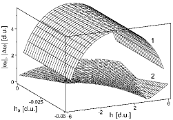
Figure 1: $|\omega_{r}|$ (surface 1) and 30$\times|\Delta\omega|$ (surface 2) as a function of $h$ and $h_{s}$ for the stationary state ($\theta_{01}$, $\varphi_{01}$).

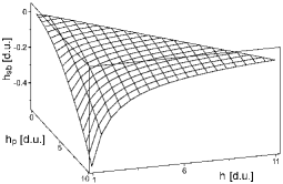
Figure 2: Spin current corresponding to the neutral, calculated as a function of $h$ and $h_{p}$.

The non-damped oscillations in the system are possible only when $1<h<1+h_{p}$ (see Ref. [gorley05, ]). This condition sets limits on the value of $h_{sb}$ as a solution of Eq. (9). Figure 2 presents a surface $h_{sb}=f(h,h_{p})$ corresponding to the parameters at which the system is in a state of non-damped magnetization oscillations, and thus being the boundary between the spin-current stable ($h_{s}>h_{sb}$) and unstable ($h_{s}<h_{sb}$) states. As follows from Fig. 2, $h_{sb}$ depends in a non-linear way on both arguments.

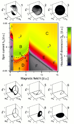
Figure 3: (Color online) Hausdorff dimension diagram $D_{H}(h,h_{s})$ for the system and the main phase portrait types for different magnetic fields $h$ and spin currents $h_{s}$: 1) $h=0.4,\,h_{s}=0.04$; 2) $h=2.825,\,h_{s}=0.02$; 3) $h=12.1,\,h_{s}=0$; 4) $h=1.1,\,h_{s}=-0.02$; 5) $h=4.125,\,h_{s}=-0.02$; 6) $h=4.5,\,h_{s}=-0.02$; 7) $h=1.075,\,h_{s}=-0.03$; 8) $h=2.925,\,h_{s}=-0.05$; 9) $h=14.25,\,h_{s}=-0.03$. Dynamic modes $A-F$ are described in the text.

Consider now numerical solutions of the nonlinear equations (1). Figure 3 presents Hausdorff dimensionhaken83 diagram $D_{H}(h,h_{s})$ showing main dynamical modes of the system (phase states) for the different applied fields and spin currents. The phase portraits corresponding to the most characteristic points of the parameter space are shown above and below the bifurcation diagram and numbered from 1 to 9. The areas $A$, $B$ and $C$ correspond to the dynamic modes, for which the transition from the initial ground state $m_{z}=-1$ to the state $m_{z}=+1$ takes place. In the area $A$ the precession of the magnetization vector takes place mainly along the axis $x$, and the phase trajectory does not cover all the unit sphere (phase portrait 1). On the contrary, the phase portraits 2 and 3, characteristic to the areas $B$ and $C$, illustrate the transition of the phase point to the upper pole via spiral trajectory, with different initial behavior of the phase point running along the two-loop curve (area $B$) or moving from the lower pole along the spiral (area $C$). Under a constant spin current and increasing magnetic field, the amplitude of the two-loop curve decreases and the phase portrait 2 (area $B$) turns into that of the phase portrait 3 (area $C$).

When the spin current decreases, the precession of the magnetization vector slows down and the phase point becomes unable to reach $m_{z}$=+1, remaining in the vicinity of the two-loop curve and becoming a limit cycle (points 4 and 5 in Fig. 3, below the upper dashed line and the corresponding phase portraits) for the magnetic fields $1<h<1+h_{p}$. Under a further decrease of the spin current, the limit cycle of the system turns into a single-loop curve (phase 6 and 7), whose form and amplitude depend on the control parameters $h$ and $h_{s}$. With a further decrease of the spin current (area $D$), the limit cycle becomes unstable and the magnetization vector instead of periodic non-damped oscillations relaxes to a certain state with negative $m_{z}$ and zero $m_{x}$ (phase portrait 8). Upon approaching $h_{lim}=1+h_{p}$, the non-stable cycle shrinks down to $m_{z}=-1$. It is worth noting that the boundary between the areas $B$ and $D$ is well-defined and sharp, contrary to the gradual transition between the areas $A-C$.

When the spin current decreases, the phase portraits corresponding to the area $C$ keep the same oscillation type, but the magnetization precession becomes significantly slower and the resulting spiral trajectory covers only a part of the unit sphere (phase portrait 9, area $E$). For the spin currents corresponding to the area $F$ (for $h<1$ and $h>1+h_{p}$), the phase point is unable to leave the ground state $m_{z}=-1$. Thus, the magnetization vector can perform non-damped oscillations, forming the phase portraits of a closed cycle for the narrow band of the control parameter values (between the dashed curves around the boundary between $B$ and $D$ in Fig. 3). Some examples of the time dependence of $m_{z}$, illustrating non-damped oscillations for the phase portraits 5, 6 and 7 are presented in Fig. 4. The curves in Fig. 4 have been plotted starting from a certain time $\tau$ to eliminate the influence of the transition processes taking place in the vicinity of $\tau$=0. As can be seen in Fig. 4(a), for a given $h_{s}$ and increasing $h$ one obtains oscillations of the lower amplitude and frequency. Increase of $h_{s}$ (Fig. 4(b), solid line) leads to the high-amplitude oscillation with smaller frequency. This indicates the possibility of controlling the period and amplitude of the non-damped oscillations of the magnetization component $m_{z}$ by the magnetic field and spin current.

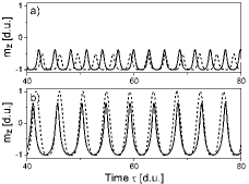
Figure 4: Time dependence of $m_{z}(\tau)$ for different magnetic fields $h$ and spin currents $h_{s}$: a) $h_{s}=-0.02$, solid line $h=4.125$, dashed line $h=4.5$; b) $h_{s}=-0.03$, solid line $h=1.075$, dashed line - calculations according to (13).

To make a qualitative description of the $m_{z}(\tau)$ behavior (Fig. 4) we use the expression for $\theta(\tau)$ from Ref. [gorley05, ], obtained in the linear approximation with respect to the perturbation,

$$\theta(\tau)=\pi+2\pi\exp(\Delta\omega)\,\sin(\omega_{r}\tau).$$ (11)

When writing Eq. (11), the initial condition $\theta(0)=\pi$ was assumed. For the non-damped oscillation mode ($\Delta\omega=0$), Eq. (11) yields

$$m_{z}(\tau)=-\cos\left[2\pi\sin(\omega_{r}\tau)\right].$$ (12)

As one may expect, the latter equation, obtained in the linear approximation, may not give good quantitative description of the essentially nonlinear $m_{z}(\tau)$ behavior, presented in Fig. 4 as a result of numerical calculations. However, one can obtain much better agreement by taking the function of the form

$$m_{z}(\tau)=-\cos\left\{2\pi\sin^{2}\left[\omega_{r0}(\tau+\tau_{0})\right]\right\},$$ (13)

where $\omega_{r0}$ and $\tau_{0}$ are some approximation parameters. For example, the $m_{z}(\tau)$ curve calculated according to (13) for $h_{s}=-0.03$, $\omega_{r0}=1.553$ and $\tau_{0}=-0.053$ (Fig. 4(b), dashed line) shows good agreement with the corresponding curve obtained by numerical methods (Fig. 4(b), solid line).

Equation (13) allows to perform a qualitative description (in the first approximation) of the possible injection of non-damped $m_{z}(\tau)$ oscillations from ferromagnetic ($F$) into non-magnetic ($N$) material. In the case of an ideal injecting contact at $x$=0, which does not change the value and orientation of the spin, one may assume that the spin currents to the left and to the right of the contact are equal,rashba00 $h_{s}^{F}=h_{s}^{N}\equiv h_{s}(0,\tau)$. In such a case, the functional dependence $h_{s}(x,\tau)$ can be obtained from the continuity equation gregg02

$$\frac{\partial m_{z}}{\partial\tau}+\frac{\partial h_{s}(x,\tau)}{\partial x}=0.$$ (14)

Introducing (13) into (14), one can show that

$$h_{s}(x,\tau)=h_{s}(0,\tau)+\pi\omega_{r0}(\xi_{+}-\xi_{-})\;x,$$ (15)

where $\xi_{\pm}=\cos\left[2\left\{\pi\sin^{2}\omega_{r0}(\tau+\tau_{0})\pm\omega_{r0}(\tau+\tau_{0})\right\}\right]$.

As follows from Eq. (15), the spin current injected from the ferromagnetic into the nonmagnetic system will preserve its non-damped oscillation character, being a superposition of the second harmonics of two harmonic oscillations. In the framework of the current assumptions it will change linearly in amplitude with distance from the contact. It is worth noting that the inclusion of relaxation item gregg02 does not change Eq. (15) qualitatively. For resistive and other contact types rashba00 ; schmidt00 ; albrecht03 , the expression for the spin current will differ from that given by Eq. (15). The results of this paper, however, show that the non-damped oscillations of $m_{z}(\tau)$ component can be injected from the ferromagnetic to a nonmagnetic system due to current continuity at the contact.

- (1) J. C. Slonczewski, J. Magn. Magn. Mater. 159, L1 (1996); 195, L261 (1999); L. Berger, Phys. Rev B 54, 9353 (1996).
- (2) J. A. Katine, et al., Phys. Rev. Lett. 84, 3149 (2000).
- (3) J. Grollier, et al., Appl. Phys. Lett. 78, 3663 (2001).
- (4) M. AlHajDarwish, et al., Phys. Rev. Lett., 93, 157203 (2004).
- (5) M. D. Stiles and A. Zangwill, Phys. Rev. B 66, 014407 (2002); J. Appl. Phys. 91, 6812 (2002).
- (6) S. I. Kiselev, et al., Nature 425, 380 (2003).
- (7) I. N. Krivorotov, et al., Science 307, 228 (2005)
- (8) J. Xiao, A. Zangwill, and M. D. Stiles, Phys. Rev. B 72, 14446 (2005).
- (9) T. Dietl, Semicond. Sci. Technol. 17, 377 (2002).
- (10) D. Ferrand, et al., Sol. State Communs. 119, 237 (2001).
- (11) E. I. Rashba, Phys. Rev. B 62, R16267 (2000).
- (12) P. M. Gorley, et al., cond-mat/0508280 (2005).
- (13) J. Z. Sun, Phys. Rev. B 62, 570 (2000).
- (14) A. Brataas, Yu. V. Nazarov, G. E. W. Bauer, Eur. Phys. J. B 22, 99, (2001).
- (15) J. Barnaś, et al., Phys. Rev. B 72, 024426 (2005).
- (16) N. P. Erugin, I. Z. Shtokalo et al. Ordinary Differential Equations (Vyshcha Shkola, Kiev, 1974).
- (17) H. Haken, Advanced Synergetics (Springer, Berlin, 1983).
- (18) J. F. Gregg, et al., J. Phys. D 35, R121 (2002).
- (19) G. Schmidt, et al., Phys. Rev. B 62, R4790 (2000).
- (20) J. D. Albrecht and D. L. Smith, Phys. Rev. B 68, 035340 (2003).