Spectral properties of disordered fully-connected graphs

Abstract

The spectral properties of disordered fully-connected graphs with a special type of the node-node interactions are investigated. The approximate analytical expression for the ensemble-averaged spectral density for the Hamiltonian defined on the fully-connected graph is derived and analysed both for the electronic and vibrational problems which can be related to the contact process and to the problem of stochastic diffusion, respectively. It is demonstrated how to evaluate the extreme eigenvalues and use them for finding the lower bound estimates of the critical parameter for the contact process on the disordered fully-connected graphs.

I Introduction

The spectral properties of complex networks are of great current interest, both for practical applications and from a fundamental point of view Dorogovtsev and Mendes (2002); Albert and Barabáshi (2002); Dorogovtsev and Mendes (2003); Fortin (2005); Iguchi and Yamada (2005a); Iguchi and Yamada (2005b); Dorogovtsev et al. (2003); Hastings (2003); Farkas et al. (2001); Goh et al. (2001); Monasson (1999); Biroli and Monasson (1999). The physical phenomena occurring in the network can be described using the operators defined for the network. For example, the Hamiltonian describes electronic excitations in the network of atoms (nodes) characterized by energy levels communicating with each other by hopping integrals (links). The Laplacian operator for a set of atoms connected by elastic springs describes vibrational excitations Maradudin et al. (1971) or transport phenomena, e.g. stochastic diffusion of random-walk type Böttger and Bryksin (1985); Rudnick and Gaspari (2004). The Liouville operator characterizes the spread of epidemics in the network Liggett (1985); Marro and Dickman (1999) and the connectivity operator gives knowledge of the network topology Dorogovtsev and Mendes (2002); Albert and Barabáshi (2002); Dorogovtsev and Mendes (2003). In the matrix representation, these operators are characterized by matrices, the eigenspectrum of which gives rather complete information of e.g. dynamical properties of the network. The main difficulty in analytical evaluation of the network spectrum is in an inherent disorder incorporated into the network matrices. This can be topological disorder related to irregular Euclidean arrangements of the nodes (e.g. atoms in liquids and glasses) and/or disorder in connectivity (complex networks e.g. of scale-free or small-world type Dorogovtsev and Mendes (2003)) or disorder in parameters associated with the nodes and links (e.g. mass and force-constant disorder for the vibrational problem on a regular lattice Taraskin and Elliott (2002) or substitutional disorder in metallic alloys Ehrenreich and Schwarts (1976)).

The first task of the spectral analysis is to evaluate the spectral density of the relevant operator for a particular realization of disorder. For an ordered system, all the realizations are identical (zero disorder) and the spectrum of at least some operators can be easily found. For disordered systems, this is a highly non-trivial problem and can be solved implicitly only for some simple models of local perturbation in a reference not necessarily ordered system (see Ref. Bogomolny et al. (2001) and references therein). The next task is to perform the averaging over different realizations of disorder (configurational averaging). The configurationally averaged spectral density can be used then for comparison with the experimentally measured spectrum (e.g. by inelastic neutron scattering for vibrational excitations Maradudin et al. (1971)) or with other observable characteristics (thermodynamical values such as heat capacity or linear response functions, e.g. the dielectric response function). Such a comparison with experimental observables makes sense if the measurable quantity is self-averaging, i.e. if the difference between the mean value of the observable for a particular realization of disorder in a macroscopically large system and the cofigurationally averaged value of this observable tends to zero with increasing system size Binder and Young (1986); Kramer and MacKinnon (1993). Some of the observables such as thermodynamical characteristics of spin glasses away from the phase transition points and of normal glasses at not very low temperatures are self-averaging. However, some of the observables such as thermodynamical characteristics of spin glasses at criticality Wiseman and Domany (1988), low temperature electron conductance Kramer and MacKinnon (1993)and dielectric response in disordered semiconductors with strong disorder Kawasaki et al. (2003) are sample-dependent and thus are not self-averaging.

The spectral density of at least Hamiltonians and Laplacians exhibits decreasing fluctuations with increasing system size (even at the localization/delocalization threshold point) and thus is expected to be a self-averaging characteristic (see e.g. van Rossum et al. (1994)). This has been seen implicitly in numerous computer simulations of spectral properties of disordered systems (see e.g. Hoffmann and Schreiber (1996) and references therein) and in experiment Elliott (1990). Usually, the ensemble averaging is tackled by means of mean-field theories Mirlin (2000); Guhr et al. (1998) with possible use of the replica method Dotsenko (2000) or introducing supersymmetry Efetov (1983); van Rossum et al. (1994) but in some cases the ”exact” solutions are available. They are quite rare and the examples are the semicircular spectrum for the fully-connected graph (FCG) with random normally distributed node-node interactions Brody et al. (1981); Mehta (1991) (see also Ref. Pastur (1972)) and Lloyd’s model for a special type of the on-site disorder and any network topology Lloyd (1960); Lehmann (1973).

The main aim of this paper is to present a model dealing with the disordered Hamiltonians defined on the FCG with a special type of the node-node interactions and a rather general type of the on-site characteristics. It is possible to find an implicit analytical expression for the spectral density for a particular realization of disorder and then to perform analytically the ensemble averaging of the spectrum of the Hamiltonian with precision up to $O(N^{-1})$ with $N$ being the number of nodes in the FCG and thus to demonstrate the self-averaging properties of the spectral density. The analytical results for the ensemble-averaged spectral density are available due to the existence of an exact solution for the matrix elements of the resolvent operator for a particular realization of disorder. The general solution is specified and analysed for several particular problems including the electronic and vibrational problems with multiplicative interactions defined on the FCG. The electronic problem is equivalent to the contact process in the dilute regime and the results can be used for the lower bound estimate of the critical point for the contact process which describes e.g. the spread of epidemics through the network. The vibrational problem is equivalent to the stochastic transport problem and the results can be used for the investigation of dynamics of information packets propagating through a communication network. The main analytical results both for the electronic and vibrational problems are supported by direct numerical diagonalization of the Hamiltonian.

The paper is organized in the following manner. The formulation of the problem is given in Sec. II. Several simple examples are considered in Sec. III followed by the general solution of the problem for polynomial interactions in Sec. IV. The limitations of the approach are discussed in Sec. V. The conclusions are made in Sec. VI and some derivations are presented in Appendices A and B.

II Formulation of the problem

Let us consider a FCG containing $N$ nodes. Each node $i$ is characterized by the parameter $\varepsilon_{i}$ (node bare energy) and the link between nodes $i$ and $j$ by parameter $V_{ij}$ (node-node interaction). Then we define an operator $\hat{\bf H}$ (”Hamiltonian”) on this FCG in the following manner,

$$\hat{\bf H}=\sum_{i}\left(\epsilon_{i}+\gamma\sum_{j\neq i}V_{ij}+V_{ii}\right)|i\rangle\langle i|-\sum_{i,j}V_{ij}|i\rangle\langle j|~{},$$ (1)

where the self-interaction matrix element $V_{ii}$ is introduced for convenience (the Hamiltonian, in fact, does not depend on it). The tuning parameter $\gamma$ gives an opportunity to distinguish between two types of problems: (i) electronic-like for $\gamma=0$ and (ii) vibrational-like when $\gamma=1$ and all $\epsilon_{i}=0$ (see also Mezard et al. (1999)). For vibrational problem, the operator $\hat{\bf H}$ is the Hessian operator and its elements obey the sum rule, $V_{ii}=\sum_{j\neq i}V_{ij}$, which follows from the global translational invariance of the Hamiltonian Maradudin et al. (1971).

Both the electronic and vibrational problems are usually defined on networks with Euclidean topology describing real materials. Below, we consider a FCG and thus the physical meaning of the Hamiltonian (1) defined on the FCG should be specified. This can be done by introducing two mappings.

First, the electronic Hamiltonian ($\gamma=0$) is equivalent to the Liouville operator, $\hat{\mathcal{L}}$, describing the contact process in the dilute regime Taraskin et al. (2005). Indeed, the time evolution of the state vector, $|P(t)\rangle$, for the contact process is governed by the master equation describing the conserved probability flow Marro and Dickman (1999), $\partial_{t}|P(t)\rangle=\hat{\mathcal{L}}|P(t)\rangle$, which can be rewritten in the dilute regime as (see Ref. Taraskin et al. (2005) for more detail)

$$\partial_{t}\overline{P}_{i}(t)=-r_{i}\overline{P}_{i}(t)+\sum_{j\neq i}W_{ji}\overline{P}_{j}(t)~{},$$ (2)

where $\overline{P}_{i}(t)$ is the probability of finding node $i$ in an occupied state independent of the occupation of all the other nodes which can be in two states, occupied (infected) or unoccupied (susceptible), $r_{i}$ is the recovery rate for node $i$ and $W_{ji}$ is the transmission (infection) rate between node $j$ and $i$. The formal solution of Eq. (2) is given by

$$|\overline{P}(t)\rangle=e^{\hat{\mathcal{L}}t}|\overline{P}(0)\rangle=\sum_{j}e^{\varepsilon_{j}t}\langle{\bf e}^{j}|\overline{P}(0)\rangle|{\bf e}^{j}\rangle~{},$$ (3)

with $\varepsilon_{j}$ and $|{\bf e}^{j}\rangle$ being the eigenvalues and eigenvectors of the Liouville operator, respectively, which coincides with the Hamiltonian (1) for $\gamma=0$, $r_{i}=-\epsilon_{i}$ and $V_{ij}=-W_{ij}$. The long-time behaviour of the contact process in the dilute regime is defined by the maximum eigenvalue, $\varepsilon_{j,{\text{max}}}$, and if $\varepsilon_{j,{\text{max}}}<0$ then the epidemic goes to extinction and it invades if $\varepsilon_{j,{\text{max}}}>0$. The approximate rate equation (2) has been obtained by replacing the term $(\overline{P}_{j}(t)-\overline{P}_{ji}(t))$ (where $\overline{P}_{ji}(t)$ is the probability for both nodes $i$ and $j$ to be occupied independent of the state of all the other nodes) in the exact equation with $\overline{P}_{j}(t)$. Such an approximation enhances the transmission of the disease and thus the estimate of the critical point obtained from the solution of the equation, $\varepsilon_{j,{\text{max}}}=0$, gives a reliable lower bound estimate of the critical parameter for the contact process meaning that if the disease does not spread in the dilute regime then it certainly does not spread in the system. This can be practically important for controlling epidemics in disordered systems where the estimate of the exact value of the critical parameter is a rather complicated task Hooyberghs et al. (2003, 2004); Vojta (2004).

The second mapping connects the vibrational problem to the problem of stochastic diffusion through a net. While the contact process describes a propagation of excitations (infected nodes) through the net with a not-conserved number of excitations (the number of infected nodes changes with time) then the standard stochastic diffusion deals with propagation of the conserved number of excitations (diffusing particles) through the net by means of diffusional jumps (characterized by the rates $W_{ij}$) between the nodes. The balance equation for stochastic diffusion coincides with Eq. (2) where $r_{i}$ is replaced by $\sum_{j\neq i}W_{ij}$ Böttger and Bryksin (1985); Webman (1981); Odagaki and Lax (1981) which reflects the conservation of the number of particles. Therefore, under the assumption of symmetric transition rates, $W_{ij}=W_{ji}$, stochastic diffusion through the network is described by the Hamiltonian (1) with $\gamma=1$, $\epsilon_{i}=0$ and $V_{ij}=-W_{ij}$. For complex networks, such as the FCG, the diffusing particles can be associated e.g. with the information packets propagating through the communication network Dorogovtsev and Mendes (2003). The quantity of interest can be e.g. the return probability of the diffusing particle to the starting place, $\langle P_{0}(t)\rangle=N^{-1}\text{Tr}\,\exp\{\hat{\bf H}t\}$ (see e.g. Friedrichs and Friesner (1988)).

The aim of our analysis is to find the eigenspectrum of Hamiltonian (1) defined on the FCG. In the site (node) basis, the Hamiltonian matrix is fully dense and, for the general case of arbitrary parameters $\epsilon_{i}$ and $V_{ij}$, its diagonalization is not a trivial task and the solution is not currently known. However, for the classical case of a random matrix belonging to the Gaussian Orthogonal Ensemble, when the off-diagonal (diagonal) elements are independent and normally distributed (with variance doubled for diagonal elements), the configurationally averaged spectrum of semicircular shape can be evaluated analytically (with errors of $O(N^{-1})$) Mehta (1991); Guhr et al. (1998). One of the key features of the matrices belonging to the Gaussian orthogonal ensemble is the statistical independence of the matrix elements.

Below, we suggest another class of real symmetric matrices for which the spectral density can be found for a particular realization of disorder and then the ensemble averaging can be performed analytically. These are matrices with a particular (polynomial) type of the node-node interactions:

$$V_{ij}=\bm{\varphi}_{i}^{T}\bm{\alpha}\bm{\varphi}_{j}~{},$$ (4)

where $\bm{\varphi}_{i}^{T}$ is a $n$-dimensional row-vector, $\bm{\varphi}_{i}^{T}=(1,\phi_{i},\phi_{i}^{2},\ldots,\phi_{i}^{n-1})$ and $\bm{\alpha}$ is a real symmetric $n\times n$ matrix of interaction coefficients, so that $V_{ij}(\phi_{i},\phi_{j})$ is a symmetric polynomial form of order $2n-2$ with respect to $\phi_{i}$ and $\phi_{j}$, e.g. $V_{ij}=\alpha_{11}+\alpha_{12}(\phi_{i}+\phi_{j})+\alpha_{22}\phi_{i}\phi_{j}$ for $n=2$. The values of $\phi_{i}$ are independent random variables characterized, in general, by different probability distribution functions, $\rho_{\phi_{i}}(\phi_{i})$. The order of interaction, $n$, is supposed to be much less than the number of nodes in the system, $n\ll N$. The diagonal elements, $\varepsilon_{i}$, in such matrices are also random independent variables distributed according to the probability distribution functions, $\rho_{\epsilon_{i}}(\epsilon_{i})$. The probability distributions $\rho_{\phi_{i}}(\phi_{i})$ and $\rho_{\epsilon_{i}}(\epsilon_{i})$ are assumed to have all finite moments unless it is stated differently.

We demonstrate below that the matrix elements of the resolvent (Green’s function) operator, $\hat{\bf G}$, defined by the equation, $(\varepsilon{\hat{\bf I}}-\hat{\bf H})\hat{\bf G}={\hat{\bf I}}$, can be found exactly for the interactions given by Eq. (4). This means, that the density of states (DOS), $g(\varepsilon)$, is available for a particular realization of disorder according to the following identity Economou (1983),

$$g(\varepsilon)=-\frac{1}{\pi N}\text{Im}~{}\text{Tr}\,{\hat{\bf G}}(\varepsilon+\text{i}0)~{}.$$ (5)

Due to the availability of the analytical expression for $g(\varepsilon)$, its configurational averaging, $\langle g(\varepsilon)\rangle$, can also be undertaken analytically by means of the following integration (for $N\to\infty$),

$$\langle g(\varepsilon)\rangle=\left\langle N^{-1}\sum_{i}\delta(\varepsilon-\varepsilon_{i})\right\rangle\equiv\idotsint N^{-1}\sum_{i}\delta(\varepsilon-\varepsilon_{i})\prod_{i}\rho_{\phi_{i}}(\phi_{i})\rho_{\epsilon_{i}}(\epsilon_{i})\,\text{d}\phi_{i}\text{d}\epsilon_{i}~{},$$ (6)

where $\varepsilon_{i}$ are the eigenvalues (eigenenergies) of the Hamiltonian.

III Simple examples

Before considering the general case of the polynomial node-node interactions (4), we present, first, three simple examples where the exact solution of the problem is available. These examples are for (i) the ideal FCG, (ii) the binary FCG and (iii) Lloyd’s model defined on the FCG. In all cases, the biological (epidemiological) applications of the results are discussed.

III.1 Ideal fully-connected graph

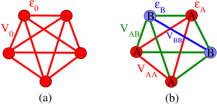
Figure 1: (Color online) Ideal (a) and binary (b) fully-connected graphs with $N=5$.

A trivial case we need as a reference for further analysis is an ideal FCG, for which all the on-site energies are identical, $\rho_{\epsilon_{i}}(\epsilon_{i})=\delta(\epsilon_{i}-\epsilon_{0})$, and all the interactions are the same, $\rho_{\phi_{i}}(\phi_{i})=\delta(\phi_{i}-\phi_{0})$ (so that $V_{ij}=V_{0}$), see Fig. 1(a). The diagonal elements of the resolvent are,

$$G_{ii}^{(0)}=\frac{N-1}{\varepsilon-\tilde{\epsilon}_{0}}+\frac{1}{\varepsilon-\tilde{\epsilon}_{0}+NV_{0}}~{},$$ (7)

where $\tilde{\epsilon}_{0}=\epsilon_{0}+V_{0}+\gamma(N-1)V_{0}$, and thus the spectrum of the ideal FCG contains two delta-functions, one of them is $(N-1)$-degenerate,

$$g_{0}(\varepsilon)=\langle g_{0}(\varepsilon)\rangle=\left(1-\frac{1}{N}\right)\delta\left(\varepsilon-\tilde{\epsilon}_{0}\right)+\frac{1}{N}\delta\left(\varepsilon-\tilde{\epsilon}_{0}+NV_{0}\right)~{}.$$ (8)

The spectrum of the Hamiltonian defined on the ideal FCG obviously obeys the ”energy-conservation” principle, $\text{Tr}\,{\hat{\bf H}}=N\epsilon_{0}$, meaning that the interactions do not change the total bare energy. If disorder is introduced in the ideal system it is quite natural to expect the broadening of the $(N-1)$-degenerate level to the band and possibly the appearance of more levels split from the band. This is exactly what happens in the disordered FCG according to the analysis presented below.

In terms of biological applications, Eq. (8) can be used for estimating the value of the critical parameter $\eta_{c}$ (this can be the ratio of the typical transmission and recovery rates) separating the absorbing ($\eta<\eta_{c}$) and active ($\eta>\eta_{c}$) states of the system with respect to the spread of the contact process (epidemic). Indeed, the maximum eigenvalue of the spectrum coincides with the position of the non-degenerate $\delta$-function and is equal to $\varepsilon_{\text{max}}=(N-1)W_{0}-r_{0}$ (bearing in mind that $\gamma=0$, $W_{0}=-V_{0}$ and $r_{0}=-\epsilon_{0}$). The solution of the equation, $\varepsilon_{\text{max}}=0$, gives a standard mean-field estimate for the critical parameter $\eta_{c}^{*}=(W_{0}/r_{0})_{c}^{*}=(N-1)^{-1}$ Marro and Dickman (1999). Obviously, if the transmission rate $W_{0}$ is $N$-independent then the critical value $\eta_{c}^{*}$ approaches zero for large values of $N$ and the system is always in the active state Dorogovtsev and Mendes (2003). However, if we assume that the transmission rate is inversely proportional to the number of nodes (in a migrating biological population the interaction time between the members of the population can be inversely proportional to the population size), $W_{0}=w_{0}/N$, with $w_{0}$ being independent of $N$, then the critical point exists and the estimate for the critical parameter is $(w_{0}/r_{0})^{*}_{c}=1$.

III.2 Binary fully connected graph

Another simple example of the network is a binary FCG (see Fig. 1(b)), for which the spectrum for a particular realization of disorder is available and configurational averaging of the DOS can be performed exactly. The binary FCG consists of nodes of two types, $A$ and $B$. The on-site energies $\epsilon_{A}$ and $\epsilon_{B}$ and the node-node interactions $V_{AA}$, $V_{BB}$ and $V_{AB}$ are defined by the types of the nodes. The node-node interactions, in general, are not of multiplicative form and can be described by Eq. (4) only if $V_{AB}^{2}=V_{AA}V_{BB}$. The only random parameter for the binary FCG is the number of nodes of a certain type, e.g. $N_{A}$, which is defined by the probability $p$ (parameter of the model) for a node to be of type $A$. The values of $N_{A}$ or equivalently of concentration $c=N_{A}/N$ are distributed according to the binomial probability distribution, $\rho_{c}(c)$ with the expectation value $E[c]=p$ and variance $\text{Var}[c]=p(1-p)N^{-1}$ which is close to the variance of the normal distribution for $N\to\infty$.

The spectral density for the electronic ($\gamma=0$) Hamiltonian (1) defined on the binary FCG characterized by a particular value of concentration $c$ contains four $\delta$-functions,

$$g(\varepsilon)=(c-N^{-1})\delta(\varepsilon-\tilde{\epsilon}_{A})+(1-c-N^{-1})\delta(\varepsilon-\tilde{\epsilon}_{B})+N^{-1}\sum_{i=1,2}\delta(\varepsilon-\varepsilon_{i})~{},$$ (9)

where $\tilde{\epsilon}_{A}=\epsilon_{A}+V_{AA}$ and $\tilde{\epsilon}_{B}=\epsilon_{B}+V_{BB}$. Only the two last $\delta$-functions,

$$g_{1}(\varepsilon)=N^{-1}\sum_{i=1,2}\delta(\varepsilon-\varepsilon_{i})~{},$$ (10)

depend on the random parameter $c\in[0,1]$ and thus should be configurationally averaged. The values of $\varepsilon_{i}$ in Eq. (10) are the roots of the spectral determinant, $D(\varepsilon_{i})=0$, where

$$D(\varepsilon)=\left(1+\frac{cNV_{AA}}{\varepsilon-\tilde{\epsilon}_{A}}\right)\left(1+\frac{(1-c)NV_{BB}}{\varepsilon-\tilde{\epsilon}_{B}}\right)-\frac{c(1-c)N^{2}V_{AB}^{2}}{(\varepsilon-\tilde{\epsilon}_{A})(\varepsilon-\tilde{\epsilon}_{B})}~{}.$$ (11)

The above expression for $D(\varepsilon)$ can be derived in a manner similar to the derivation for multiplicative interactions (see Appendix A).

For simplicity, we consider a symmetric binary FCG characterized by $\epsilon_{A}=\epsilon_{B}=\epsilon_{0}=-r_{0}$ and $V_{AA}=V_{BB}=V_{0}$ and also assume that the node-node interactions are negative and inversely proportional to $N$, so that the interaction parameters, $w=-NV_{0}\,$ and $\lambda=-NV_{AB}$, are positive and $N$-independent. In this case, the $c-\varepsilon$ map defined by the equation, $D(\varepsilon)=0$, with $D(\varepsilon)$ obeying Eq. (11), is given by the following bilinear form,

$$(\varepsilon+r_{0}-w/2)^{2}+(\lambda^{2}-w^{2})(c-1/2)^{2}=\lambda^{2}/4~{},$$ (12)

where we have ignored the terms $\propto N^{-1}$. Therefore, the positions of the $\delta$- functions in Eq. (10) can be found as the roots of Eq. (12) for a particular value of $c$,

$$\varepsilon_{1,2}=-r_{0}+\frac{w}{2}\pm\sqrt{\frac{\lambda^{2}}{4}-(\lambda^{2}-w^{2})\left(c-\frac{1}{2}\right)^{2}}~{},$$ (13)

The form (12) is hyperbolic for a weak interaction ($\lambda<w$) between subgraphs $A$ and $B$ and elliptic for strong coupling ($\lambda>w$). The configurational averaging in Eq. (10) is straightforward and

$$\langle g_{1}(\varepsilon)\rangle=\frac{N^{-1}|\varepsilon+r_{0}-w/2|}{\sqrt{(\lambda^{2}-w^{2})(\lambda^{2}/4-(\varepsilon+r_{0}-w/2)^{2})}}\left[\rho_{c}(c_{1})+\rho_{c}(c_{2})\right]~{},$$ (14)

where $c_{1,2}=1/2\pm\left[(\lambda^{2}/4-(\varepsilon+r_{0}-w/2)^{2})/(\lambda^{2}-w^{2})\right]^{1/2}$. The analysis of Eq. (14) shows that, for any finite $N$, two $\delta$-functions are broadened by disorder into two bands separated by a gap of width $W_{g}=\lambda$ for weak coupling and $W_{g}=w$ for strong coupling (see Fig. 6(a) and (b), respectively). The non-linearity of the map results in the singular behaviour of the ensemble-averaged DOS around $\varepsilon=-r_{0}+w/2\pm\lambda/2$ where $\langle g_{1}(\varepsilon)\rangle\propto(\varepsilon+r_{0}-w/2\mp\lambda/2)^{-1/2}$.

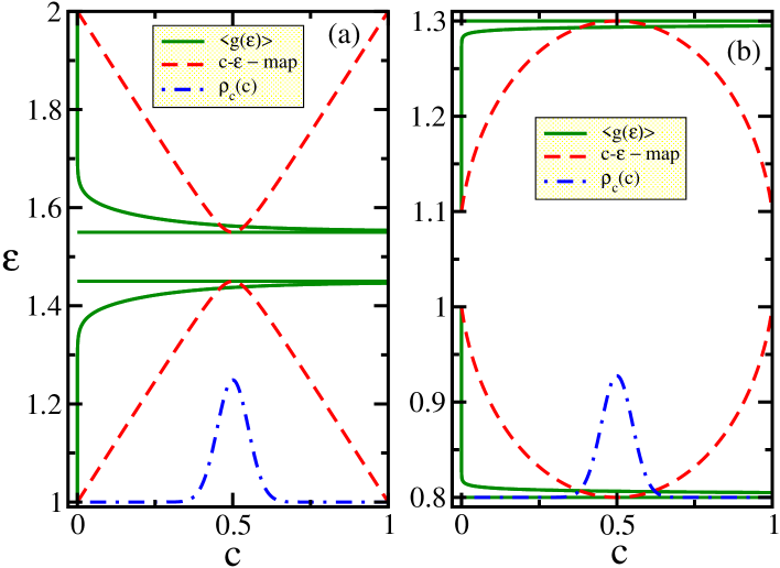
Figure 2: (Color online) The $c-\varepsilon$ map (dashed line) for the symmetric binary FCG in the regime of weak (a) and strong (b) coupling. The ensemble-averaged DOS (scaled), $\langle g_{1}(\varepsilon)\rangle$, and the probability distribution function (scaled), $\rho_{c}(c)$, are shown by the solid and dot-dashed lines, respectively. The values of the parameters are: (a) $\epsilon_{0}=1$, $w=1$ and $\lambda=0.1$; (b) $\epsilon_{0}=1$, $w=0.1$ and $\lambda=0.5$. The probability $p=0.5$ and $N=100$ for both regimes.

The ensemble-averaged spectrum for the binary FCG is bounded from the top by energy, $\varepsilon_{\text{max}}$, the knowledge of which is quite important from the applicational viewpoint (see below). The value of $\varepsilon_{\text{max}}$ is easy to find from Eqs. (12), (14) and it is

$$\varepsilon_{\text{max}}=-r_{0}+w~{}~{}~{}\text{for}~{}~{}~{}\lambda<w~{},$$ (15)

and

$$\varepsilon_{\text{max}}=-r_{0}+\frac{1}{2}(w+\lambda)~{}~{}~{}\text{for}~{}~{}~{}\lambda>w~{}.$$ (16)

Eqs. (15)-(16) give the upper boundaries for the maximum eigenvalues for a particular realization of disorder, i.e. for a particular value of $c$. In the limit of large values of $N\to\infty$, the binomial distribution $\rho_{c}(c)$ is of the Gaussian form characterized by the negligible width and thus it approaches the $\delta$-functional peak. Consequently, both energy bands collapse into two $\delta$-functions located at $\varepsilon=\varepsilon_{1,2}$ given by Eq. (13) and $\varepsilon_{\text{max}}\simeq\varepsilon_{1}$. Therefore, the critical value of parameter $\eta=w/r_{0}$ can be found from the solution of equation, $\varepsilon_{1}=0$. In the limit of weak coupling between the subgraphs, $\lambda<w$, the critical value $\eta_{c}^{*}$ depends on $c$ and lies in the interval, $1\leq\eta_{c}^{*}\leq 2/(1+\lambda/w)$. The value of $\eta_{c}^{*}$ reaches the maximum, $\eta_{c}^{*}=2/(1+\lambda/w)$, for the homogeneous FCG, when $c=0$ (FCG contains only nodes of type $B$) or $c=1$ (FCG contains only nodes of type $A$). The minimum, $\eta_{c}^{*}=1$, is attained for equal concentrations of nodes $A$ and $B$, i.e. when $c=0.5$. In the regime of strong coupling between subgraphs, $\lambda>w$, the situation changes to the opposite one so that $2/(1+\lambda/w)\leq\eta_{c}^{*}\leq 1$ and the lowest value of $\eta_{c}^{*}$ corresponds to $c=0.5$.

Biologically, this means that mixed populations containing two species are most vulnerable to epidemics for equal concentrations of species if these species strongly interact with each other (in terms of transferring disease) and if the species do not interact strongly enough then the mixture of species enhances the resistance of the population.

The above estimates hold for the populations of organisms which are able to communicate (transfer a disease) to all other members of the population, i.e. for populations having the communication network with the topology of the FCG. The other assumption is that the transmission rate between two individuals is inversely proportional to the number of individuals in the population. This is a plausible assumption for migrating individuals when the probability to establish a contact can be proportional to $N^{-1}$.

III.3 Lloyd’s model

It is known that the configurational averaging of the spectral density can be performed analytically for the network of any topology, and thus for the FCG as well, if the diagonal elements of the Hamiltonian matrix are distributed according to the Cauchy distribution,

$$\rho_{\epsilon_{i}}(\epsilon_{i})=\rho_{\epsilon}(\epsilon_{i})=\frac{\delta}{\pi}\,\frac{1}{\delta^{2}+(\epsilon_{i}-\epsilon_{0})^{2}}~{},$$ (17)

where $\delta$ is the width of the distribution, and all the relevant node-node interactions are not random, $V_{ij}=V_{0}$ (Lloyd’s model Lloyd (1960)).

The diagonal elements of the configurationally-averaged resolvent operator, $\langle G_{ii}(\varepsilon)\rangle$ can be expressed via the resolvent elements for the ideal FCG, $G_{ii}^{(0)}$, with the argument shifted to the upper half of the complex plane, $\langle G_{ii}(\varepsilon)\rangle=G_{ii}^{(0)}(\varepsilon+\text{i}\delta)$. Therefore the ensemble-averaged spectral density for Lloyd’s model defined on the FCG has the following form:

$$\langle g(\varepsilon)\rangle=\left(1-\frac{1}{N}\right)\rho_{\epsilon}(\varepsilon-V_{0}-\gamma(N-1)V_{0})+\frac{1}{N}\rho_{\epsilon}(\varepsilon-(\gamma-1)(N-1)V_{0})~{},$$ (18)

i.e. the DOS is obtained from that for the ideal FCG by broadening of both $\delta$-functions in Eq. (8) into two Lorentzian peaks. Formally, the FCG with on-site energies distributed according to the Cauchy distribution is equivalent to the ideal FCG with nodes characterized by the complex on-site energies (see also Neut and Speicher (1995)).

In contrast to the binary FCG, the widths of both of the Lorentzian peaks in Eq. (18) do not depend on $N$ and for any value of $\delta$ it is possible to find such a value of $N$ starting from which the positive eigenvalues appear in the spectrum. This means that Lloyd’s model on the FCG is not resistant to the invasion of epidemics at least in the dilute regime. It is a consequence of the special form of the distribution of the recovery rates given by Eq. (17) with not existing high moments.

IV Polynomial interactions

We have considered above several simple examples of the FCG for which the spectrum can be found exactly and its configurational averaging can be performed analytically. A natural question arises about the possibility of a similar analysis in the case of more general disorder. Below, we demonstrate that indeed in the case of the polynomial node-node interactions such an analysis is possible.

IV.1 General Solution

In the case of the polynomial node-node interactions for the FCG, the matrix elements of the resolvent operator in the site basis can be found exactly and the spectral density for a particular realization of disorder is given by the following formula (see Appendix A):

$$g(\varepsilon)=g_{0}(\varepsilon)+\delta g(\varepsilon)=\frac{1}{N}\sum_{i}^{N}\delta(\varepsilon-\widetilde{\epsilon}_{i})-\frac{1}{\pi N}\text{Im}\,\frac{\text{d}}{\text{d}\varepsilon}\left[\ln\left(\text{det}\,{\bf D}(\varepsilon)\right)\right]~{}.$$ (19)

Here the renormalized bare energies, $\widetilde{\epsilon}_{i}$, are given by Eq. (43) and the spectral determinant, $\text{det}\,{\bf D}(\varepsilon)$, satisfies Eq. (48).

Assuming for simplicity that all $\epsilon_{i}$ and $\phi_{i}$ are identically distributed according to the probability distribution functions $\rho_{\epsilon_{i}}(\epsilon_{i})\equiv\rho_{\epsilon}(\epsilon_{i})$ and $\rho_{\phi_{i}}(\phi_{i})\equiv\rho_{\phi}(\phi_{i})$, respectively, the spectral density $g(\varepsilon)$ can be configurationally averaged according to Eq. (6),

$$\langle g(\varepsilon)\rangle = \langle g_{0}(\varepsilon)\rangle+\langle\delta g(\varepsilon)\rangle$$ (20)

$$= \int\limits_{-\infty}^{\infty}\rho_{\phi}(\phi_{i})\rho_{\epsilon}(\epsilon-\widetilde{V}_{ii})\,\text{d}\phi_{i}-\frac{1}{\pi N}\,\frac{\text{d}}{\text{d}\varepsilon}\left\langle\text{arg}\,\left(\text{det}\,{\bf D}(\varepsilon)\right)\right\rangle~{},$$

where

$$\widetilde{V}_{ii}=\gamma\bm{\psi}_{i}^{T}\sum_{j}^{N}\bm{\varphi}_{j}+(1-\gamma)\bm{\psi}_{i}^{T}\bm{\varphi}_{i}\simeq\gamma N\bm{\psi}_{i}^{T}\overline{\bm{\varphi}}+(1-\gamma)\bm{\psi}_{i}^{T}\bm{\varphi}_{i}~{},$$ (21)

with $\bm{\psi}_{i}^{T}=\bm{\varphi}_{i}^{T}\bm{\alpha}$ and $\overline{\bm{\varphi}}=\int_{-\infty}^{\infty}\bm{\varphi}_{i}\rho_{\phi}(\phi_{i})\,\text{d}\phi_{i}$ so that $\widetilde{V}_{ii}$ depends on the characteristics of node $i$ only (see below for the justification of this approximation). The ensemble-averaged spectral density, $\langle g(\varepsilon)\rangle$, has two contributions. The first contribution, $\langle g_{0}(\varepsilon)\rangle$, is given by the convolution of two probability distributions, one of them, $\rho_{\epsilon}$, is shifted along the energy axis due to the node-node interactions. If both distributions $\rho_{\epsilon}$ and $\rho_{\phi}$ are band-shaped (e.g. normal, box or $\delta$-functional distributions) then the function $\langle g_{0}(\varepsilon)\rangle$ also has the shape of a band of typical width $\Delta$ defined via the widths of the distributions $\rho_{\epsilon}$ and $\rho_{\phi}$.

The other contribution to the spectral density comes from $\langle\delta g(\varepsilon)\rangle$ and its magnitude is negligible in the main band region (due to the factor $N^{-1}$ in Eq. (20)) and finite outside the band with $\langle\delta g(\varepsilon)\rangle$ being in the form of several peaks (see below). The functional form of $\langle\delta g(\varepsilon)\rangle$ depends on the properties of the spectral determinant $\text{det}\,{\bf D}$. It follows from Eq. (48), that the spectral determinant is a random value which depends only on macroscopic sums, $a_{k}=\sum_{i}^{N}a_{ki}=\sum_{i}^{N}\phi_{i}^{k}(\varepsilon-\tilde{\epsilon}_{i})^{-1}$, i.e. $\text{det}\,{\bf D}=D(\varepsilon;a_{0},a_{1},\ldots,a_{2n-2})$. According to the central limit theorem, the values of $a_{k}$ are distributed around the mean value $\overline{a_{k}}\simeq N\overline{a_{ki}}$ in the peak region of width $\delta a_{k}\simeq\left(N\text{Var}[a_{ki}]\right)^{1/2}$, i.e. the relative peak width of this distribution approaches zero in the thermodynamic limit ($N\to\infty$), $\delta a_{k}/\overline{a_{k}}\propto N^{-1/2}\to 0$. Bearing this in mind we can perform configurational averaging of the phase of the spectral determinant in Eq. (20) approximately (assuming, in fact, that the spectral density is a self-averaging quantity),

$$\left\langle\text{arg}\,\left(\text{det}\,{\bf D}(\varepsilon;a_{0},a_{1},\ldots,a_{2n-2})\right)\right\rangle\simeq\text{arg}\,\left(\text{det}\,{\bf D}(\varepsilon;\overline{a_{0}},\overline{a_{1}},\ldots,\overline{a_{2n-2}})\right)~{},$$ (22)

where

$$\overline{a_{k}(\varepsilon)} = N\iint\limits_{-\infty}^{\infty}\frac{\phi_{i}^{k}}{\varepsilon-\epsilon_{i}-\widetilde{V}_{ii}(\phi_{i})}\,\rho_{\epsilon}(\epsilon_{i})\rho_{\phi}(\phi_{i})\,\text{d}\epsilon_{i}\,\text{d}\phi_{i}$$ (23)

$$= N\int\limits_{-\infty}^{\infty}\phi_{i}^{k}R(\varepsilon-\widetilde{V}_{ii}(\phi_{i}))\,\text{d}\phi_{i}+\text{i}N\int\limits_{-\infty}^{\infty}\phi_{i}^{k}I(\varepsilon-\widetilde{V}_{ii}(\phi_{i}))\,\text{d}\phi_{i}~{},$$

with

$$R(z)=\diagup\hskip-15.0pt\int\limits_{-\infty}^{\infty}\,\frac{\rho_{\epsilon}(\epsilon_{i})}{z-\epsilon_{i}}\,\text{d}\epsilon_{i}~{}~{}~{}~{}\text{and}~{}~{}~{}~{}I(z)=-\pi\rho_{\epsilon}(z)~{}.$$ (24)

Eq. (22) becomes exact for an infinite number of nodes. Note that the same arguments were used in the derivation of Eq. (21) for replacing $\sum_{j}^{N}\bm{\varphi}_{j}$ with $N\overline{\bm{\varphi}}$ resulting in $\widetilde{V}_{ii}$ being a function of $\phi_{i}$ only but not other $\phi_{j}$ for $j\neq i$.

Expressing the phase, $\text{arg}\,\left(\text{det}\,{\bf D}(\varepsilon;\overline{a_{0}},\overline{a_{1}},\ldots,\overline{a_{2n-2}})\right)$, via real and imaginary parts of the spectral determinant, $D=\widetilde{D}+\text{i}\widetilde{\widetilde{D}}$, and differentiating it with respect to energy according to Eq. (20) we arrive at the following final expression for $\langle g(\varepsilon)\rangle$,

$$\langle g(\varepsilon)\rangle=\langle g_{0}(\varepsilon)\rangle+\langle\delta g(\varepsilon)\rangle\simeq\int\limits_{-\infty}^{\infty}\rho_{\phi}(\phi_{i})\rho_{\epsilon}(\epsilon-\widetilde{V}_{ii})\,\text{d}\phi_{i}-\frac{1}{\pi N}\,\frac{\widetilde{D}\left.\widetilde{\widetilde{D}}\right.^{\prime}-\left.\widetilde{D}\right.^{\prime}\widetilde{\widetilde{D}}}{\left.{\widetilde{D}}\right.^{2}+\left.\widetilde{\widetilde{D}}\right.^{2}}~{},$$ (25)

where prime means differentiation with respect to $\varepsilon$. This is the main result of the paper. Eq. (25) allows the spectral density of the FCG with polynomial interactions to be calculated for rather general distributions of the bare energies, $\epsilon_{i}$, and interaction characteristics, $\phi_{i}$. The functional form of the spectral determinant $D(\varepsilon)$ depends on a concrete formulation of the problem but it is irrelevant for the main band shape and can influence only the positions of discrete levels split from the main band. An alternative derivation of Eq. (25) by means of direct integration of the left-hand side of Eq. (22) (and thus demonstrating the self-averaging property for the spectral density) is presented in Appendix B for multiplicative interactions in the electronic case.

In the band region, where the contribution from $\langle g_{0}(\varepsilon)\rangle$ is significant, both functions $\widetilde{D}(\varepsilon)$ and $\widetilde{\widetilde{D}}(\varepsilon)$ are typically of the same order of magnitude, $\widetilde{D}\sim\widetilde{\widetilde{D}}$ and $\left.\widetilde{D}\right.^{\prime}\sim\left.\widetilde{\widetilde{D}}\right.^{\prime}\sim\widetilde{D}/\Delta$ (if $n\ll N$), so that the contribution from $\langle\delta g(\varepsilon)\rangle$ to the total ensemble-averaged spectral density is macroscopically small, $\langle\delta g(\varepsilon)\rangle\sim(N\Delta)^{-1}$. This is not surprising and is a consequence of the particular form of the node-node interactions given by Eq. (4) forcing the majority of the eigenvalues, $\varepsilon_{i}$, of the Hamiltonian (1) (the roots of the spectral determinant, $D(\varepsilon_{i})=0$) to be bound between the consequent renormalized bare energies, i.e. $\varepsilon_{i}\in(\widetilde{\epsilon}_{j},\widetilde{\epsilon}_{j+1})$. This property is similar to the well-known phenomenon of the spectral reconstruction caused by the interactions of one level (e.g. associated with the defect) with a continuum of levels (band) (see e.g. Refs.  Maradudin et al. (1971); Lehmann (1973); Bohr and Mottelson (1989); Klinger and Taraskin (1993); Bogomolny et al. (2001) and the discussion in Sec. IV.2).

Outside the main band region, where $\widetilde{\widetilde{D}}\to 0$, the function $\langle\delta g(\varepsilon)\rangle$ contributes in the form of the Gaussian peaks (see the explanation below), $\langle\delta g(\varepsilon)\rangle=\sum_{i=1}^{m}N(E[\varepsilon_{*i}],\text{Var}[\varepsilon_{*i}])$, of width $\delta\varepsilon_{*i}=\sqrt{\text{Var}[\varepsilon_{*i}]}$ and centred around the expectation value, $E[\varepsilon_{*i}]$ (the function $N(E[x],\text{Var}[x])$ stands for the normal distribution of $x$ with the expectation value $E[x]$ and variance $\text{Var}[x]$). The peak locations coincide with the roots of the real part of the spectral determinant, $\widetilde{D}(E[\varepsilon_{*i}])=0$, and the number of roots, $m$, cannot exceed the order of the spectral determinant, i.e. the order of interactions, $m\leq n$. Indeed, for energies far away from the band, ${\cal E}/\Delta\gg 1$ where ${\cal E}=|\varepsilon-\overline{\epsilon}-\overline{\widetilde{V}_{jj}}|$ (where $\overline{\widetilde{V}_{jj}}=\int\widetilde{V}_{jj}\rho_{\phi}(\phi_{j})\text{d}\phi_{i}$ and $\overline{\epsilon}=\int\epsilon_{i}\rho_{\epsilon}(\epsilon_{i})\text{d}\epsilon_{i}$), we can estimate the value of $\overline{a}_{k}\sim N\overline{\phi^{k}}/{\cal E}$, so that the spectral determinant is the $n$-th order polynomial of $(N/{\cal E})$ with constant finite coefficients (under the assumption that the interaction coefficients $\alpha_{ij}$ do not depend on $N$). It can have maximum $n$ of $N$-independent roots, so that $|\varepsilon_{*i}-\overline{\epsilon}-\overline{\widetilde{V}_{jj}}|\propto N$. This means that the Gaussian peaks are mainly macroscopically separated from the band.

Therefore, the interactions of polynomial type (4) change the bare spectrum $\epsilon_{i}$ of the Hamiltonian (1) in the following manner: (i) the bare band is shifted and deformed and (ii) several isolated levels macroscopically separated from the band are formed. Such a picture will be supported below by detailed analysis of some simple cases of the low-order interactions for $n=2$.

IV.2 Multiplicative interactions for the electronic problem

We start the analysis with the simplest case of multiplicative (separable) node-node interactions, when the second-order interaction matrix contains only one non-zero element, $\alpha_{22}$, so that

$$V_{ij}=\left(1~{}~{}\phi_{i}\right)\left(\begin{array}[]{cc}0{}&~{}0\\ 0{}&~{}\alpha_{22}\end{array}\right)\left(\begin{array}[]{c}1\\ \phi_{j}\end{array}\right)=\alpha_{22}\phi_{i}\phi_{j}~{}.$$ (26)

The spectral determinant for a particular realization of disorder is

$$D(\varepsilon)=1+\sum_{i}^{N}\frac{\alpha_{22}\phi_{i}^{2}}{\varepsilon-\tilde{\epsilon}_{i}}~{},$$ (27)

with

$$\tilde{\epsilon}_{i}=\epsilon_{i}+\widetilde{V}_{ii}\simeq\epsilon_{i}+\gamma\alpha_{22}N\phi_{i}\overline{\phi}+(1-\gamma)\alpha_{22}\phi_{i}^{2}~{}.$$ (28)

We consider below the electronic problem ($\gamma=0$) mainly but the general results for arbitrary values of $\gamma$ will be presented when possible.

The roots of the spectral determinant, $\varepsilon_{i}$, are bound between the renormalized bare energies, $\varepsilon_{i}\in(\tilde{\epsilon}_{i-1},\tilde{\epsilon}_{i})$ (for $\alpha_{22}>0$) which is obvious from the functional form of $D(\varepsilon)$ given by Eq. (27). Therefore the eigenvalues of the Hamiltonian are expected to be very close to the renormalized bare energies, $\varepsilon_{i}=\tilde{\epsilon_{i}}+O(\Delta/N)$, and the changes in the spectral density within the band region for $\tilde{\epsilon_{i}}$ due to interactions (26) should be negligible ($\propto N^{-1}$). This property is very similar to Rayleigh’s theorem in the theory of vibrations in disordered systems Maradudin et al. (1971).

The ensemble-averaged spectral density is given by Eq. (25) with

$$\widetilde{D}(\varepsilon;\overline{a_{2}})=1+\text{Re}\,\overline{a_{2}(\varepsilon)}=1+N\int\limits_{-\infty}^{\infty}\alpha_{22}\phi_{i}^{2}R(\varepsilon-\widetilde{V}_{ii})\,\text{d}\phi_{i}~{},$$ (29)

and

$$\widetilde{\widetilde{D}}(\varepsilon;\overline{a_{2}})=\text{Im}\,\overline{a_{2}(\varepsilon)}=N\int\limits_{-\infty}^{\infty}\alpha_{22}\phi_{i}^{2}I(\varepsilon-\widetilde{V}_{ii})\,\text{d}\phi_{i}~{},$$ (30)

where the functions $R(z)$ and $I(z)$ are defined by Eq. (24). The properties of the function $\langle g(\varepsilon)\rangle$ have already been discussed above. In particular, in the main-band region the contribution from $\langle\delta g(\varepsilon)\rangle$ is negligible ($\propto(N\Delta)^{-1}$) while outside the band it can exhibit Gaussian peaks. For multiplicative interactions, there is only one Gaussian peak outside the band, $\langle g(\varepsilon)\rangle\simeq\langle\delta g(\varepsilon)\rangle\simeq N(\varepsilon_{*},\sigma^{2})$, with the peak position being the solution of the following equation $\widetilde{D}(\varepsilon_{*})=0$, i.e.

$$1+N\int\limits_{-\infty}^{\infty}\alpha_{22}\phi_{i}^{2}R(\varepsilon_{*}-\widetilde{V}_{ii})\,\text{d}\phi_{i}=0~{}.$$ (31)

This equation can be solved approximately assuming that the level $\varepsilon_{*}$ is split from the band far enough in comparison with the band width, i.e. $\left|\varepsilon_{*}-\overline{\epsilon}-\overline{\widetilde{V}_{ii}}\right|/\Delta\gg 1$,

$$\varepsilon_{*}\simeq\overline{\epsilon}-N\alpha_{22}\overline{\phi^{2}}~{}.$$ (32)

Indeed, we see from Eq. (32) that the distance between the isolated level and the main band is macroscopically large, $\propto N$ (if the coefficient $\alpha_{22}$ does not depend on $N$), which is consistent with the result for the ideal FCG (see Eq. (8)) showing the similar structure of the spectrum with the $(N-1)$-degenerate level playing the role of the main band.

In order to estimate the width of the Gaussian peak, we consider a particular $j$-th realization of disorder for which the random value of $\varepsilon_{j*}$ can be estimated in a similar manner, $\varepsilon_{j*}\simeq N^{-1}\sum_{i}^{N}\epsilon_{i}-\alpha_{22}\sum_{i}^{N}\phi_{i}^{2}$. From this expression according to the central limit theorem, we conclude that the values of $\varepsilon_{j*}$ are normally distributed with the expectation value given by Eq. (32) and with variance,

$$\sigma^{2}\simeq\frac{\text{Var}[\epsilon_{i}]}{N}+N\alpha_{22}^{2}\text{Var}[\phi_{i}^{2}]~{}.$$ (33)

This expression for the variance coincides with that given by Eq. (73) more rigorously derived in Appendix B. It follows from Eq. (33) that the peak width, $\sigma$, depends on $N$ and it increases with $N$, $\sigma\propto\sqrt{N}$, if the interaction coefficient $\alpha_{22}$ does not depend on $N$. However, if $\alpha_{22}\propto 1/N$, the peak width decreases with $N$, $\sigma\propto 1/\sqrt{N}$, and the peak collapses to a $\delta$-function in the thermodynamic limit.

All the results presented above for the multiplicative interactions are supported in Appendix B by an alternative derivation of Eqs. (25), (29)-(30) for the ensemble-averaged spectral density using direct approximate integration of Eq. (6).

Numerical analysis confirms all the conclusions made above. Fig. 3 demonstrates both the main band (a) and the Gaussian peak (b) for the case of multiplicative interactions for the electronic problem ($\gamma=0$) defined on the FCG. It is clearly seen how the interactions shift the Gaussian bare band (dot-dashed curve in Fig. 3(a)) and change its shape. The isolated level is normally distributed (see Fig. 3(b)) and macroscopically shifted down along the energy axis. For all cases, the results of direct diagonalization are practically indistinguishable from those obtained in accord with analytical expressions.

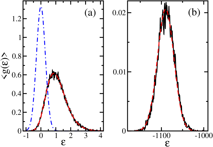
Figure 3: (Color online) The ensemble-averaged DOS (the main band, $\langle g(\varepsilon)\rangle\simeq\langle g_{0}(\varepsilon)\rangle$, in (a) and separate level, $\langle g(\varepsilon)\rangle\simeq\langle\delta g(\varepsilon)\rangle$, outside the main band in (b)) for electron problem ($\gamma=0$) defined on the FCG with multiplicative interactions. Both the on-site energies $\epsilon_{i}$ and interaction parameters $\phi_{i}$ are normally distributed according to $\rho_{\epsilon}(\epsilon_{i})=N(0,0.09)$ (the dot-dashed line in Fig. 1(a)) and $\rho_{\phi}(\phi_{i})=N(1,0.09)$; $\alpha_{22}=1$. The dashed lines in (a) and (b) are plotted according to the first term in Eq. (25) and Eqs. (72)-(73), respectively. The solid lines represent the data obtained by direct diagonalization of the Hamiltonian for $N=1000$ nodes and averaging over $10^{4}$ configurations. The DOS in Fig. 3(b) is scaled by factor $N$.

The evaluation of the integral in the expression for $\langle g_{0}(\varepsilon)\rangle$ (see Eq. (25)) has been performed numerically in the above example illustrated in Fig. 3. Such an integration becomes trivial if one of the probability distribution functions is a $\delta$-function. For example, if the on-site energies are randomly distributed while the interactions are all the same, $\rho_{\phi}(\phi_{i})=\delta(\phi_{i}-\phi_{0})$, the configurationally averaged spectral density coincides with the shifted distribution of the on-site energies, $\langle g_{0}(\varepsilon)\rangle=\rho_{\epsilon}(\varepsilon-\alpha_{22}\phi_{0}^{2})$ (due to the linear map between $\epsilon_{i}$ and $\varepsilon$, i.e. $\varepsilon=\tilde{\epsilon}_{i}=\epsilon_{i}+\alpha_{22}\phi_{0}^{2}$ which follows from Eq. (28)). On the other hand, the on-site energies can be all the same, $\rho_{\epsilon}(\epsilon_{i})=\delta(\epsilon_{i}-\epsilon_{0})$, but the interactions are randomly distributed. In this case, due to the quadratic map between $\phi_{i}$ and $\varepsilon$, i.e. $\varepsilon=\tilde{\epsilon}_{i}=\epsilon_{0}+\alpha_{22}\phi_{i}^{2}$ (see Eq. (28)), there are two contributions to the ensemble-averaged DOS from different branches of this quadratic map (see Fig. 4),

$$\langle g_{0}(\varepsilon)\rangle=\frac{1}{2\sqrt{\alpha_{22}(\varepsilon-\epsilon_{0})}}\left[\rho_{\phi}\left(\sqrt{\frac{\varepsilon-\epsilon_{0}}{\alpha_{22}}}\right)+\rho_{\phi}\left(-\sqrt{\frac{\varepsilon-\epsilon_{0}}{\alpha_{22}}}\right)\right]~{}.$$ (34)

with $\varepsilon$ obeying the following inequality, $\alpha_{22}(\varepsilon-\epsilon_{0})>0$. The ensemble-averaged DOS exhibits a singular behaviour around the boundary of the spectrum at $\varepsilon\simeq\epsilon_{0}$ (see Fig. 5),

$$\langle g_{0}(\varepsilon)\rangle\simeq\frac{\rho_{\phi}(0)}{\sqrt{\alpha_{22}(\varepsilon-\epsilon_{0})}}~{},$$ (35)

if $\rho_{\phi}(0)$ is a finite non-zero value. From this example, we see that the bare spectral density can display quite drastic changes in shape depending on the type and probability distribution of the interaction parameters.

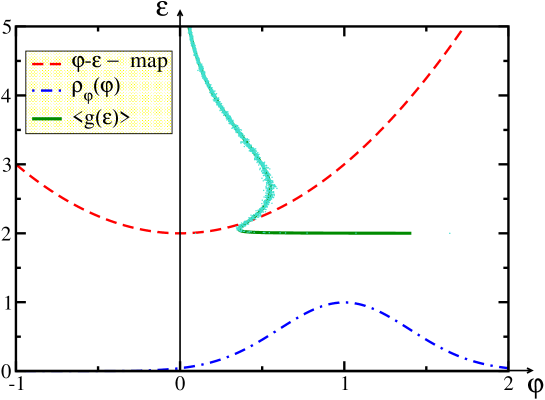
Figure 4: (Color online) The $\phi-\varepsilon$ parabolic map (dashed line) for the electron problem ($\gamma=0$) defined on the FCG with multiplicative interactions ($\epsilon_{0}=2$, $\alpha_{22}=1$). The interaction parameters are normally distributed according to $\rho_{\phi}(\phi_{i})=N(1,0.16)$. The ensemble-averaged DOS (scaled), $\langle g(\varepsilon)\rangle\simeq\langle g_{0}(\varepsilon)\rangle$, and the probability distribution function (scaled), $\rho_{\phi}(\phi_{i})$, are shown by the solid (Eq. (34)) and dot-dashed lines, respectively. The dots scattered around the solid line were obtained by direct diagonalization of the Hamiltonian ($N=3000$) and by averaging over 300 realizations of disorder.

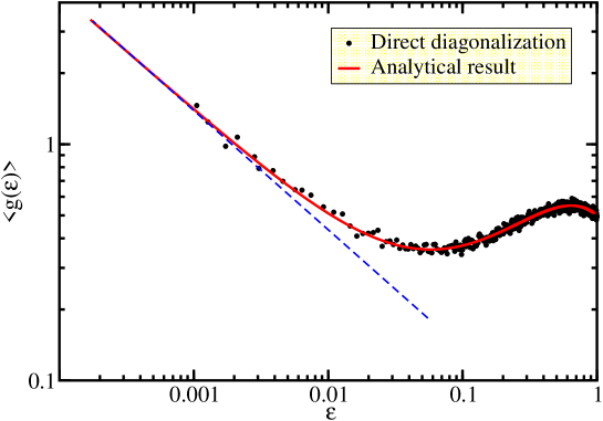
Figure 5: (Color online) The double-log plot of $\langle g(\varepsilon)\rangle\simeq\langle g_{0}(\varepsilon)\rangle$ shown in Fig. 4 around the singularity. The solid line was obtained using Eq. (35) and the dots represent the results of direct diagonalization. The dashed line, $\propto\varepsilon^{-1/2}$, is used as an eye guide.

In terms of epidemiological applications, the above analysis can be used for an estimate of the critical parameter $\eta_{c}$. Indeed, the low-bound estimate for $\eta_{c}$ can be easily obtained for the FCG with polynomial interactions by finding the position of the largest isolated eigenvalue, $\varepsilon_{*}^{\text{max}}$, and solving the equation, $\varepsilon_{*}^{\text{max}}(\eta_{c}^{*})=0$ with $\varepsilon_{*}^{\text{max}}$ being the largest root of the real part of the spectral determinant, $\widetilde{D}(\varepsilon_{*}^{\text{max}})=0$. An important and general conclusion which follows from the analysis presented above is that the isolated normally distributed roots of the real part of the spectral determinant scale linearly with $N$, i.e. $\varepsilon_{*}^{\text{max}}\propto N$ if the interaction coefficients, $\alpha_{ij}$, and the interaction parameters, $\phi_{i}$, and thus the transmission rates, $W_{ij},$ do not depend on $N$. This means that equation $\varepsilon_{*}^{\text{max}}(\eta_{c}^{*})=0$ does not have the solution independent of $N$ and the system does not exhibit the phase transition in the thermodynamic limit (it is always in the active state). In the opposite case, when the transmission rates are inversely proportional to $N$, the maximum eigenvalue does not depend on $N$ and the transition exists at least for the Hamiltonian in the dilute regime. The concrete value of the critical parameter $\eta_{c}^{*}$ depends on the particular type of the interactions and the probability distributions for recovery and transmission rates.

IV.3 Multiplicative interactions for the vibrational problem

For vibrational problem defined on the FCG ($\gamma=1$ and $\epsilon_{i}=0$) with multiplicative interactions, the ensemble-averaged DOS is given by Eq. (25) with $\rho_{\epsilon_{i}}(\epsilon_{i})=\delta(\epsilon_{i})$ and

$$\tilde{\epsilon}_{i}=\alpha_{22}N\phi_{i}\overline{\phi}\equiv\beta\phi_{i}\overline{\phi}~{},$$ (36)

where $\beta=\alpha_{22}N$. Eq. (36) reveals the linear map between $\phi_{i}$ and $\varepsilon$, i.e. $\varepsilon=\tilde{\epsilon}_{i}=\beta\phi_{i}\overline{\phi}$, and thus for the main band,

$$\langle g_{0}(\varepsilon)\rangle=\frac{1}{|\beta\overline{\phi}|}\rho_{\phi}\left(\frac{\varepsilon}{\beta\overline{\phi}}\right)~{}.$$ (37)

If the coefficient $\alpha_{22}$ does not depend on $N$ then $\beta\propto N$ and the location of the main band $\langle g_{0}(\varepsilon)\rangle$ also scales with $N$. In the opposite case of $\beta$ being independent of $N$, the ensemble-averaged spectral density is $N$-independent. Fig. 6 illustrates the high quality of the approximate expression for $\langle g_{0}(\varepsilon)\rangle\simeq\langle g(\varepsilon)\rangle$ in the band region (the solid line in Fig. 6) by comparison with the results obtained by direct diagonalization of the Hamiltonian matrix (the dashed line in Fig. 6).

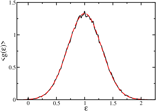
Figure 6: (Color online) The ensemble-averaged DOS for the vibrational problem ($\gamma=1$) defined on the FCG with multiplicative interactions. The random interaction parameters $\phi_{i}$ are normally distributed according to $\rho_{\phi}(\phi_{i})=N(1,0.09)$; $\beta=1$. The dashed line is plotted according to Eq. (37) and the data for the solid line are obtained by direct diagonalization of the Hamiltonian for $N=3000$ nodes and averaging over 50 configurations.

Similarly to the electronic problem, the contribution of $\langle\delta g(\varepsilon)\rangle$ to the spectral density is negligible ($\propto 1/N$) in the main band region. A specific feature of the vibrational problem is that one of the peak-shaped contributions from $\langle\delta g(\varepsilon)\rangle$ is always of the $\delta$-functional form at exactly zero energy. For the multiplicative interactions, this is the only peak-shaped contribution, i.e. $\langle\delta g(\varepsilon)\rangle=N^{-1}\delta(\varepsilon)$. This is a consequence of the global translational invariance of the Hamiltonian and also follows from the solution of the equation $\widetilde{D}(\varepsilon_{*})=0$, which reads

$$\widetilde{D}(\varepsilon_{*})=1+\diagup\hskip-15.0pt\int\limits_{-\infty}^{\infty}\frac{\beta\phi_{i}^{2}}{\varepsilon_{*}-\beta\overline{\phi}\phi_{i}}\rho_{\phi}(\phi_{i})\text{d}\phi_{i}=0~{}.$$ (38)

Obviously, the value of $\varepsilon_{*}=0$ is the solution of Eq. (38) and thus the peak is located at zero energy. This statement holds for an arbitrary realization of disorder, when the integrals in Eq. (38) should be replaced by finite sums and thus the peak associated with $\varepsilon_{*}$ is of $\delta$-functional form.

Therefore, the vibrational problem defined on the FCG with multiplicative interactions has a relatively simple ensemble-averaged spectral density. It contains the main band which is obtained by rescaling of the probability distribution for interaction parameters and a $\delta$-functional peak at zero energy.

The results obtained for the vibrational problem can be applied to the investigation of the transport properties of communication networks characterized by symmetric transmission rates $W_{ij}=-V_{ij}\geq 0$ (i.e. $\beta<0$) and $W_{ij}=W_{ji}$. For example, the above analysis for separable node-node interactions is applicable for a network with communication channels charcterized by multiplicative functions Guimera et al. (2002). In this case, the dynamical characteristics of a packet propagating through the network crucially depend on the functional form of the distribution, $\rho_{\phi}(\phi_{i})$, of the interaction parameters $\phi_{i}$. One of these characteristics is the return probability, $\langle P_{0}(t)\rangle$, of the packet to the starting point of its diffusion through the network (see e.g. Friedrichs and Friesner (1988)),

$$\langle P_{0}(t)\rangle=N^{-1}\text{Tr}\,\exp\{\hat{\bf H}t\}=\int\limits_{-\infty}^{\infty}e^{\varepsilon t}\langle g_{0}(\varepsilon)\rangle\text{d}\varepsilon+\frac{1}{N}~{},$$ (39)

where $\langle g_{0}(\varepsilon)\rangle$ is given by Eq. (37). The spectrum of the Hamiltonian (1) is negative except for one eigenvalue located exactly at zero which gives rise to the last term in Eq. (39) describing the random return of the packet to the origin. The time dependence of the return probability is dictated by the functional form of $\rho_{\phi}(\phi)$ in Eq. (37). If the distribution $\rho_{\phi}(\phi)$ has the form of a band, $\phi\in\left[\phi_{\text{min}},\phi_{\text{max}}\right]$, separated from zero by a gap, i.e. $\phi_{\text{min}}>0$, then the long-time behaviour of the first term in Eq. (39) for the return probability is exponential, $\langle P_{0}(t)\rangle\propto\exp(-\beta\overline{\phi}\phi_{\text{min}}t)$. On the other hand, if the distribution of $\phi$ starts from zero with $\rho_{\phi}(\phi\to 0)\propto\phi^{\alpha}$ with $\alpha>-1$, the return probability decays with time according to the power law, $\langle P_{0}(t)\rangle\propto t^{-\alpha-1}$ for large times. This property can be quite important for monitoring the localization properties of the information packets by means of choosing the appropriate distribution for the interaction parameters $\phi_{i}$.

IV.4 Polynomial interactions of higher orders

To conclude this section about polynomial interactions defined on the FCG, we should emphasise that there are no principal difficulties in extending the above analysis to the cases of higher-order interactions with $n>2$. The features of the ensemble-averaged spectral density will be the same as for the multiplicative interactions. The shape of the main band can vary significantly depending on the order of interaction and the probability distributions of the bare energies and interaction parameters.

A typical example is shown in Fig. 7 for the electronic problem ($\gamma=0$) defined on the FCG with polynomial interactions of order $n=6$ characterized by a normal distribution of the interaction parameters and a $\delta$-functional distribution of the bare energies. In this case, the convolution of the probability distributions in Eq. (25) is trivial and the band shape is dictated by the non-linear $\phi-\varepsilon$ map (see the inset in Fig. 7) given by the polynomial of order $2n-1$ with the singularities in the DOS being due to the extremal points in the $\phi-\varepsilon$ map. The ensemble-averaged DOS calculated according to Eq. (25) (the dashed line) is practically identical to the exact one (the solid line) obtained by direct diagonalization of the Hamiltonian. The isolated levels, $\varepsilon_{i*}$, can be found if necessary by solving the equation for the real part of the spectral determinant, $\widetilde{D}(\varepsilon_{i*})=0$.

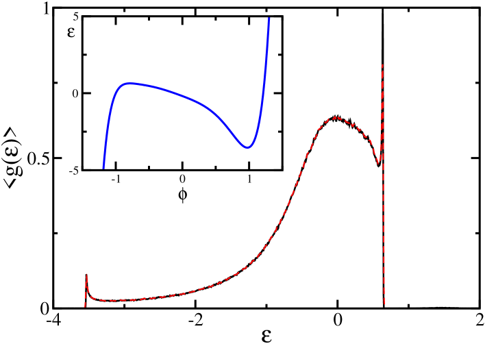
Figure 7: (Color online) The exact (solid line) and approximate (the dashed line) ensemble-averaged DOS (over $10^{3}$ realizations) for the FCG ($N=3000$) with node-node interactions defined by Eq. (4) in which $n=6$. The elements of the $\bm{\alpha}$-matrix are random values withdrawn from the uniform distribution defined in the interval, $\alpha_{ij}\in[-1,1]$. The on-site energies and interaction parameters are distributed according to $\rho_{\epsilon}(\epsilon)=\delta(\epsilon)$ and $\rho_{\phi}(\phi)=N(0,0.16)$, respectively. The non-linear $\phi-\varepsilon$ map is shown in the inset.

V Limitations

In the previous section, we have demonstrated that the evaluation of the spectral density and its configurational averaging for the Hamiltonian defined on the FCG can be performed analytically in some special cases. Namely, this can be done for the binary FCG exactly and approximately for the FCG with a particular polynomial type of the node-node interactions. One of the restrictions for the polynomial interactions is that the order of interactions must be much less than the number of nodes in the FCG, $n\ll N$. Generally speaking the solution given by Eq. (25) is valid for arbitrary value of $n$ but it becomes ”useless” for $n\gtrsim N$ in the sense that the conclusions made above about the structure of $\langle g(\varepsilon)\rangle$ do not necessarily hold for this case. For example, the maximum number of levels split from the main band due to polynomial interactions should be less or equal to the order of interactions, $n$, and therefore it can reach the value of $N$ if $n\gtrsim N$. This means that the main band described by $\langle g_{0}(\varepsilon)\rangle$ in Eq. (25) can disappear completely and a new band or set of levels arises due to the contribution from $\langle\delta g(\varepsilon)\rangle$ (see an example below). The positions of levels split from the main band should be found by solving the $n$-th order polynomial for the real part of the spectral determinant. The complexity of this problem is not less than that of the original eigenproblem and thus solution (25) becomes not very informative.

The condition $n\ll N$ can be broken for a very important type of the node-node interactions, $V_{ij}=V(|\phi_{i}-\phi_{j}|)$, depending on Euclidean distance, $|\phi_{i}-\phi_{j}|$, between nodes, where the $\phi_{i}$ play the role of the node coordinates which can be random values (for simplicity, we analyse one-dimensional space). For example, let us consider a set of nodes randomly displaced from the sites in the ideal linear chain, so that ($E[\phi_{j}]=ja$; $a$ is the mean distance between nearest sites and $j$ is an integer). Assume also that the node-node interactions decay exponentially with the distance,

$$V_{ij}=V_{0}\exp\{-[\beta(\phi_{i}-\phi_{j})]^{2}\}~{},$$ (40)

where $\beta$ is the inverse interaction length and $V_{0}$ is a constant. The interactions $V_{ij}$ given by Eq. (40) can be expanded in a Taylor series generally containing an infinite number of terms and thus presented in the form of Eq. (4) with $n\gg N$.

However, in the case of long-range interactions when the typical interaction length, $\beta$, is comparable to the system size, $L$, i.e. $\beta^{-1}\gtrsim L=Na$, the Taylor series for $V_{ij}$ contains only a finite number of terms, $n\ll N$, and the interactions are of the polynomial type. Consequently, the ensemble-averaged spectral density should be well approximated in the main band region by the function $\langle g_{0}(\varepsilon)\rangle$ evaluated according to Eq. (25) which gives for the electronic problem,

$$\langle g_{0}(\varepsilon)\rangle=\rho_{\epsilon}(\varepsilon-V_{0})~{},$$ (41)

because $\tilde{\epsilon}_{i}=\epsilon_{i}+V_{ii}=\epsilon_{i}+V_{0}$. It follows from Eq. (41) that $\langle g_{0}(\varepsilon)\rangle$ does not depend on the distribution of $\phi_{i}$ at all. Indeed, we have found numerically that in the case of long-range interactions the ensemble-averaged spectral density follows the theoretical prediction (41) (the black curve in Fig. 7 obtained by direct diagonalization for $\beta Na=1$ is indistinguishable from that obtained using Eq. (41)). In this regime, all the nodes interact with each other at approximately the same strength, $V_{ij}\simeq V_{0}$, and the system is equivalent to the FCG with on-site energy disorder only.

When the typical interaction length decreases, more terms in the Taylor series for $V_{ij}$ should be kept for the accurate representation of function (40) leading to an increase in the order of the polynomial interactions. An increase in the value of $n$ gives rise to more and more levels split down off the main band (see the red solid curve in Fig. 8 for $\beta Na=10^{2}$). These separate levels eventually form a broad band for medium-range interactions (see the dark green dashed curve in Fig. 8 for $\beta Na=5\times 10^{2}$) which transforms to a relatively narrow band of width, $\Delta\simeq 4V_{0}\exp(-\beta^{2}a^{2})$, having a well-recognizable shape of a band for the spectrum of an ideal linear chain with nearest-neighbour interactions broadened by diagonal and off-diagonal disorder (see the blue double-dot-dashed and light green solid curves in Fig. 8 for $\beta Na=10^{3}$ and $\beta Na=1.5\times 10^{3}$, respectively). The original main band centred around $\varepsilon\simeq\overline{\varepsilon}+V_{0}$ for long-range interactions eventually disappears with increasing value of $\beta$.

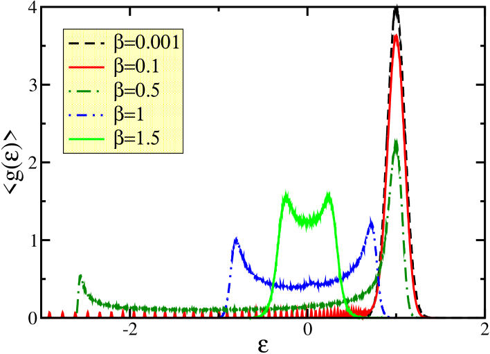
Figure 8: (Color online) The exact ensemble-averaged DOS (over $3\times 10^{3}$ configurations) for a linear chain on $N=10^{3}$ nodes interacting with each other according to Eq. (40) ($V_{0}=1$ and $a=1$) for different values of the inverse interaction length $\beta$ (as marked). The on-site energies and interaction parameters are normally distributed according to $\rho_{\epsilon}(\epsilon)=N(0,0.01)$ and $\rho_{\phi}(\phi)=N(1,0.01)$, respectively.

Therefore, we can conclude that the theory for polynomial interactions presented in Sec. IV can be applied to systems with Euclidean long-range interactions but fails to describe the short-range interactions.

The other limitation of the above analysis concerns its applicability to the disordered complex networks of the FCG topology only. Of course, the topology of real complex networks is much more complicated (e.g. scale-free or small-world topologies Dorogovtsev and Mendes (2003)) and the FCG can be considered as a first approximation for the networks with high node-node connectivity.

VI Conclusions

To conclude, we have analysed the spectral properties of the Hamiltonian both for electronic and vibrational problems defined on the fully-connected graphs with a special type (polynomial) of interactions.

Our main finding is the analytical formula (see Eq. 25) for the ensemble-averaged spectral density. The ensemble-averaged spectral density has two contributions with clear physical interpretations: (i) the first contribution describes the main spectral band and (ii) the second one is related to the set of discrete levels separated from the band. The main band originates from the bare spectral band shifted and deformed by means of a convolution of two probability distributions of bare energies and interaction parameters. The discrete levels are split from the bare spectral band due to interactions and the number of such levels depends on the order of the interactions.

The approximate analytical configurational averaging is possible due to the availability of the exact analytical solution for the resolvent matrix elements for a particular realization of disorder (see Appendix A). Technically, configurational averaging is done with the use of the central limit theorem by replacing the function of fluctuating macroscopic sums by the function of the means of these sums (see Eq. 22). This step can be justified and illustrated by a more rigorous approach for a particular case (see Appendix B). All the final results are convincingly supported by numerics.

Both the electronic and vibrational problems discussed in the paper can be mapped to the contact process in the dilute regime and the stochastic diffusion problem, respectively. The results for the electronic case can thus be used for obtaining the lower bound estimate of the critical parameter for the contact process while the results for the vibrational case allow the return probability for an information packet to be evaluated for the communication networks.

Appendix A Exact solution for the resolvent matrix elements

The resolvent matrix elements for the Hamiltonian given by Eq. (1) can be found exactly for the node-node interactions of polynomial type  (4). In order to demonstrate this let us recast the equation for the resolvent, $(\varepsilon{\hat{\bf I}}-\hat{\bf H})\hat{\bf G}={\hat{\bf I}}$, as

$$G_{ij}=\frac{\delta_{ij}}{\varepsilon-\tilde{\epsilon}_{i}}-\frac{1}{\varepsilon-\tilde{\epsilon}_{i}}\sum_{k}\bm{\psi}_{i}^{T}\bm{\varphi}_{k}G_{kj}~{},$$ (42)

where the renormalized bare energy, $\tilde{\epsilon}_{i}$, is

$$\tilde{\epsilon}_{i}=\epsilon_{i}+\gamma\bm{\psi}_{i}^{T}\sum_{j}^{N}\bm{\varphi}_{j}+(1-\gamma)\bm{\psi}_{i}^{T}\bm{\varphi}_{i}=\epsilon_{i}+\widetilde{V}_{ii}~{},$$ (43)

with $\bm{\psi}_{i}^{T}=\bm{\varphi}_{i}^{T}\bm{\alpha}$. The value of $\widetilde{V}_{ii}=\gamma\bm{\psi}_{i}^{T}\sum_{j}^{N}\bm{\varphi}_{j}+(1-\gamma)\bm{\psi}_{i}^{T}\bm{\varphi}_{i}=\epsilon_{i}+\widetilde{V}_{ii}$ generally depends on all $\phi_{j}$ but $\widetilde{V}_{ii}=V_{ii}(\phi_{i})$ for the electronic problem ($\gamma=0$).

The node-separable type of polynomial interactions in Eq. (4) ($i-j$ interaction is proportional to the matrix product of separate node characteristics) allows factorization to be performed there by introducing $\bf{x}_{j}=\sum_{k}\bm{\varphi}_{k}G_{kj}$, so that

$$G_{ij}=\frac{\delta_{ij}}{\varepsilon-\tilde{\epsilon}_{i}}-\frac{1}{\varepsilon-\tilde{\epsilon}_{i}}\bm{\psi}_{i}^{T}\bf{x}_{j}~{}.$$ (44)

Eq. (42) can be multiplied by $\bm{\varphi}_{i}$ and summed over $i$ and thus transformed to equation which can be solved for $\bf{x}_{j}$,

$$\bf{x}_{j}=\left(\bf{I}+\sum_{i}^{N}\frac{\bm{\varphi}_{i}\bm{\psi}_{i}^{T}}{\varepsilon-\tilde{\epsilon}_{i}}\right)^{-1}\frac{\bm{\varphi}_{j}}{\varepsilon-\tilde{\epsilon}_{j}}~{},$$ (45)

Substitution of $\bf{x}_{j}$ into Eq. (44) results in the required result for the resolvent matrix elements,

$$G_{ij}=\frac{\delta_{ij}}{\varepsilon-\tilde{\epsilon}_{i}}-\frac{\bm{\psi}_{i}^{T}}{\varepsilon-\tilde{\epsilon}_{i}}\left(\bf{I}+\sum_{k}^{N}\frac{\bm{\varphi}_{k}\bm{\psi}_{k}^{T}}{\varepsilon-\tilde{\epsilon}_{k}}\right)^{-1}\frac{\bm{\varphi}_{j}}{\varepsilon-\tilde{\epsilon}_{j}}~{}.$$ (46)

The DOS is expressed via $\text{Tr}\hat{\bf G}$, which is given by the following expression,

$$\text{Tr}\hat{\bf G}=\sum_{i}^{N}\frac{1}{\varepsilon-\tilde{\epsilon}_{i}}-\sum_{i}^{N}\frac{\bm{\psi}_{i}^{T}}{\varepsilon-\tilde{\epsilon}_{i}}{\bf D}^{-1}\frac{\bm{\varphi}_{i}}{\varepsilon-\tilde{\epsilon}_{i}}~{},$$ (47)

and

$${\bf D}=\left(\bf{I}+\sum_{k}^{N}\frac{{\bm{\varphi}}_{k}{\bm{\psi}}_{k}^{T}}{\varepsilon-\tilde{\epsilon}_{k}}\right)~{},$$ (48)

The eigenvalues, $\varepsilon_{i}$, of the Hamiltonian coincide with the poles of the resolvent which are the roots of the spectral determinant, $D(\varepsilon)=\text{det}\,{\bf D}(\varepsilon)|$, i.e. $D(\varepsilon_{i})=0$. This follows from the form of Eq. (47) in which the contributions to the denominator from the first sum, $\propto(\varepsilon-\tilde{\epsilon}_{i})$, are cancelled by the similar terms in Eq. (47).

It is easy to show that Eq. (47) can be recast in an elegant form via the derivative of the spectral determinant,

$$\text{Tr}\hat{\bf G}=\sum_{i}^{N}\frac{1}{\varepsilon-\tilde{\epsilon}_{i}}+\frac{\text{d}\ln[\text{det}({\bf D})]}{\text{d}\varepsilon}~{}.$$ (49)

Indeed, rewriting the second term from Eq. (47) in the following form,

$$\sum_{i}^{N}\frac{\bm{\psi}_{i}^{T}}{\varepsilon-\tilde{\epsilon}_{i}}{\hat{\bf D}}^{-1}\frac{\bm{\varphi}_{i}}{\varepsilon-\tilde{\epsilon}_{i}}=[\text{det}({\bf D})]^{-1}\sum_{i}^{N}\sum_{k,m}^{n}\frac{(\bm{\psi}_{i}^{T})_{k}}{\varepsilon-\tilde{\epsilon}_{i}}C_{mk}\frac{(\bm{\varphi}_{i})_{m}}{\varepsilon-\tilde{\epsilon}_{i}}~{},$$ (50)

where ${\bf C}$ stands for the matrix of cofactors for matrix ${\bf D}$, and comparing it with the derivative of $\text{det}({\bf D})$,

$$\frac{\text{d}\,\text{det}({\bf D})}{\text{d}\varepsilon}=\sum_{m,k}\frac{\text{d}D_{mk}}{\text{d}\varepsilon}C_{mk}=-\sum_{m,k}\frac{(\bm{\varphi}_{i})_{m}(\bm{\psi}_{i}^{T})_{k}}{(\varepsilon-\tilde{\epsilon}_{i})^{2}}C_{mk}~{},$$ (51)

we arrive at Eq. (49). Finally, taking the imaginary part of Eq. (49) and using then Eq. (5) leads to Eq. (19).

Appendix B Configurational averaging by direct integration

In this Appendix, we give an alternative derivation of the expression for the ensemble-averaged spectral density in the case of the multiplicative node-node interaction, $V_{ij}=\alpha_{22}\phi_{i}\phi_{j}$, for the random Hamiltonian defined on the FCG. The derivation is similar in some aspects to that given in Ref. Bogomolny et al. (2001) for the mean density of eigenvalues of a 2D integrable billiard.

The starting point for the derivation is Eq. (47) recasted for the multiplicative interaction (26) in the following form:

$$\text{Tr}\hat{\bf G} = \sum_{i}^{N}\frac{1}{\varepsilon-\tilde{\epsilon}_{i}}\,-\,\sum_{i}^{N}\frac{\alpha_{22}\phi_{i}^{2}}{(\varepsilon-\tilde{\epsilon}_{i})^{2}}\left(1+\sum_{i}^{N}\frac{\alpha_{22}\phi_{i}^{2}}{\varepsilon-\tilde{\epsilon}_{i}}\right)^{-1}$$ (52)

$$= \sum_{i}^{N}\frac{1}{\varepsilon-\tilde{\epsilon}_{i}}\,-\,\text{i}\sum_{i}^{N}\frac{\alpha_{22}\phi_{i}^{2}}{(\varepsilon-\tilde{\epsilon}_{i})^{2}}\int\limits_{-\infty}^{0-}e^{\text{i}k\left(1+\sum_{i}^{N}\frac{\alpha_{22}\phi_{i}^{2}}{\varepsilon-\tilde{\epsilon}_{i}}\right)}\text{d}k~{},$$

where

$$\tilde{\epsilon_{i}}=\epsilon_{i}+\alpha_{22}\phi_{i}^{2}~{},$$ (53)

for the electronic problem ($\gamma=0$) analysed below for concreteness (the analysis can be easily extended to the vibrational problem ($\gamma=1$)). Using definition (5) and Eq. (6) we obtain the expression for $\langle g(\varepsilon)\rangle=\langle g_{0}(\varepsilon)\rangle+\langle\delta g(\varepsilon)\rangle$, where $\langle g_{0}(\varepsilon)\rangle$ coincides with the first integral term in Eq. (20) with $V_{ii}=\alpha_{22}\phi_{i}^{2}$ and $\langle\delta g(\varepsilon)\rangle$ is given by

$$\langle\delta g(\varepsilon)\rangle=\frac{1}{\pi N}\,\text{Re}\,\int\limits_{-\infty}^{0-}e^{\text{i}k}\text{d}k\idotsint\sum_{j}^{N}\frac{\alpha_{22}\phi_{j}^{2}}{(\varepsilon-\tilde{\epsilon}_{j})^{2}}\prod_{i}e^{\text{i}k\frac{\alpha_{22}\phi_{i}^{2}}{\varepsilon-\tilde{\epsilon}_{i}}}\rho_{\phi}(\phi_{i})\rho_{\epsilon}(\epsilon_{i})\text{d}\phi_{i}\text{d}\epsilon_{i}~{},$$ (54)

or by the equivalent expression (assuming for definiteness that $\alpha_{22}>0$),

$$\langle\delta g(\varepsilon)\rangle=\frac{1}{\pi}\text{Re}\,\int\limits_{-\infty}^{0-}e^{\text{i}k}\left[F(k,\varepsilon)\right]^{N-1}Q(k,\varepsilon)\text{d}k~{},$$ (55)

with

$$F(k,\varepsilon)=\int\limits_{-\infty}^{\infty}\rho_{\phi}(\phi_{i})f(\phi_{i},k,\varepsilon)\text{d}\phi_{i}=\int\limits_{-\infty}^{\infty}\rho_{\phi}(\phi_{i})\int\limits_{-\infty}^{\infty}e^{\text{i}k\frac{\alpha_{22}\phi_{i}^{2}}{\varepsilon-\tilde{\epsilon}_{i}}}\rho_{\epsilon}(\epsilon_{i})\text{d}\epsilon_{i}\text{d}\phi_{i}~{},$$ (56)

and

$$Q(k,\varepsilon)=\int\limits_{-\infty}^{\infty}\rho_{\phi}(\phi_{i})q(\phi_{i},k,\varepsilon)\text{d}\phi_{i}=\int\limits_{-\infty}^{\infty}\rho_{\phi}(\phi_{i})\int\limits_{-\infty}^{\infty}\frac{\alpha_{22}\phi_{i}^{2}}{(\varepsilon-\tilde{\epsilon}_{i})^{2}}e^{\text{i}k\frac{\alpha_{22}\phi_{i}^{2}}{\varepsilon-\tilde{\epsilon}_{i}}}\rho_{\epsilon}(\epsilon_{i})\text{d}\epsilon_{i}\text{d}\phi_{i}~{},$$ (57)

where the function $q(\phi_{i},k,\varepsilon)$ is related to $f(\phi_{i},k,\varepsilon)$ by the following equation,

$$q(\phi_{i},k,\varepsilon)=-\frac{1}{\alpha_{22}\phi_{i}^{2}}\,\frac{\partial^{2}f(\phi_{i},k,\varepsilon)}{\partial k^{2}}~{}.$$ (58)

The next step is in the evaluation of the integral,

$$f(\phi_{i},k,\varepsilon)=\int\limits_{-\infty}^{\infty}e^{-\text{i}\frac{\chi}{z-\epsilon_{i}}}\rho_{\epsilon}(\epsilon_{i})\text{d}\epsilon_{i}~{},$$ (59)

($\chi\equiv-k\alpha_{22}\phi_{i}^{2}>0$) with the integrand exhibiting an essential singular point at $\epsilon_{i}=\varepsilon+\text{i}0-\alpha_{22}\phi_{i}^{2}\equiv z$. This can be done by expanding the exponential function in a Taylor series and integrating each term,

$$f = \int\limits_{-\infty}^{\infty}\rho_{\epsilon}(\epsilon_{i})\left[1-\text{i}\chi\,\frac{1}{z-\epsilon_{i}}+\frac{(\text{i}\chi)^{2}}{2}\,\frac{1}{(z-\epsilon_{i})^{2}}+\cdots\right]\text{d}\epsilon_{i}$$ (60)

$$= 1-\text{i}\chi\left(R(z)+\text{i}I(z)\right)+\frac{\chi^{2}}{2}\left(R^{\prime}(z)+\text{i}I^{\prime}(z)\right)+O(\chi^{3}/\Delta^{3})~{},$$

where the functions $R(z)$ and $I(z)$ are defined by Eq. (24). In order to evaluate the third term in Eq. (60) we integrated once by parts and used the following identity,

$$R^{\prime}(z)=\diagup\hskip-15.0pt\int\limits_{-\infty}^{\infty}\frac{\rho_{\epsilon}(z)-\rho_{\epsilon}(\epsilon_{i})}{(z-\epsilon_{i})^{2}}\text{d}\epsilon_{i}=\diagup\hskip-15.0pt\int\limits_{-\infty}^{\infty}\frac{\rho_{\epsilon}^{\prime}(\epsilon_{i})}{z-\epsilon_{i}}\text{d}\epsilon_{i}~{}.$$ (61)

In expansion (60), we keep only the terms up to the second order in $\beta/\Delta$ including because this is enough for obtaining the leading term for $q(\phi_{i},k,\varepsilon)$ according to Eq. (58)

$$q(\phi_{i},k,\varepsilon)=-\alpha_{22}\phi_{i}^{2}\left[R^{\prime}(\varepsilon-\alpha_{22}\phi_{i}^{2})+\text{i}I^{\prime}(\varepsilon-\alpha_{22}\phi_{i}^{2})\right]~{}.$$ (62)

The higher order terms in $\beta/\Delta$ are small both for $f(\phi_{i},k,\varepsilon)$ and $q(\phi_{i},k,\varepsilon)$ because typical values of $|k|$ significantly contributing into integral (55) in the band region are $|k|\sim\Delta/(\alpha_{22}\phi_{i}^{2}N)$ (see below) and thus $\beta/\Delta\sim 1/N\ll 1$. Note, that the same result for $f(\phi_{i},k,\varepsilon)$ can be obtained by a different method based on the shift of the essential singularity to infinity as was suggested in Ref. Bogomolny et al. (2001).

Substitution of Eqs. (61)-(62) into Eqs. (56)-(57) gives,

$$F(k,\varepsilon) = 1+\text{i}k\left[R_{1}(\varepsilon)+\text{i}I_{1}(\varepsilon)\right]+\frac{k^{2}}{2}\left[R_{2}^{\prime}(\varepsilon)+\text{i}I_{2}^{\prime}(\varepsilon)\right]$$ (63)

$$Q(k,\varepsilon) = -R_{1}^{\prime}(\varepsilon)-\text{i}I_{1}^{\prime}(\varepsilon)~{},$$ (64)

where

$$R_{m}(k,\varepsilon) = \int\limits_{-\infty}^{\infty}\rho_{\phi}(\phi_{i})\left[\alpha_{22}\phi_{i}^{2}\right]^{m}R(\varepsilon-\alpha_{22}\phi_{i}^{2})\text{d}\phi_{i}$$ (65)

$$I_{m}(k,\varepsilon) = \int\limits_{-\infty}^{\infty}\rho_{\phi}(\phi_{i})\left[\alpha_{22}\phi_{i}^{2}\right]^{m}I(\varepsilon-\alpha_{22}\phi_{i}^{2})\text{d}\phi_{i}~{}.$$ (66)

Using the above expressions for $F(k,\varepsilon)$ and $Q(k,\varepsilon)$ we can rewrite Eq. (55) as

$$\langle g(\varepsilon)\rangle=-\frac{1}{\pi}\text{Re}\left\{\left[R_{1}^{\prime}(\varepsilon)+\text{i}I_{1}^{\prime}(\varepsilon)\right]\int\limits_{-\infty}^{0-}e^{\psi(k)}\text{d}k\right\}~{},$$ (67)

with

$$\psi(k)=\text{i}k+(N-1)\ln\left[1+k(\text{i}R_{1}-I_{1})+\frac{k^{2}}{2}(R_{2}^{\prime}+\text{i}I_{2}^{\prime}\right]$$ (68)

$$= \text{i}k(1+NR_{1})-kNI_{1}+\frac{k^{2}N}{2}\left(R_{1}^{2}+R_{2}^{\prime}-I_{1}^{2}\right)+\frac{\text{i}k^{2}N}{2}\left(I_{2}^{\prime}+2R_{1}I_{1}\right)+O(k^{3})~{}.$$

There are two energy regions: (i) inside the band where $R_{m}(\varepsilon)\sim I_{m}(\varepsilon)\sim\alpha_{22}^{m}\overline{\phi^{m}}/\Delta$ and (ii) outside the band where $R_{m}(\varepsilon)\sim\alpha_{22}^{m}\overline{\phi^{m}}/|\varepsilon_{*}-\overline{\epsilon}|$ with $|\varepsilon_{*}-\overline{\epsilon}|\gg\Delta$ and $I_{m}(\varepsilon)$ either approaches zero (e.g. exponentially for the normal distribution $\rho_{\epsilon}$) or identically equals zero for the box distribution. In these regions, integral (67) has different contributions to the total ensemble-averaged spectral density. Inside the band, we can ignore the terms $\propto k^{2}$ in expression (68) for $\psi(k)$, so that $e^{\psi(k)}$ exponentially decays for $|k|\to\infty$ on the typical scale $k\sim 1/(NI_{1})\sim\Delta/(\alpha_{22}\overline{\phi^{2}}N)$, and

$$\langle\delta g(\varepsilon)\rangle=-\frac{1}{\pi N}\frac{(1+NR_{1})NI_{1}^{\prime}-NR_{1}^{\prime}NI_{1}}{(1+NR_{1})^{2}+(NI_{1})^{2}}~{},$$ (69)

which exactly coincides with the second term in Eq. (25) bearing in mind that $\widetilde{D}=1+NR_{1}$ and $\widetilde{\widetilde{D}}=NI_{1}$.

Outside the band, $\rho_{\epsilon}\to 0$ and thus $I_{m}\to 0$, so that the real linear term in $k$ in Eq. (68) becomes negligible and the next terms in the expansion must be kept,

$$\psi(k)\simeq\text{i}k(1+NR_{1})+\frac{k^{2}N}{2}\left(R_{1}^{2}+R_{2}^{\prime}\right)~{},$$ (70)

where

$$R_{2}^{\prime}\simeq-\iint\left[\frac{\alpha_{22}\phi_{i}^{2}}{\varepsilon-\alpha_{22}\phi_{i}^{2}-\epsilon_{i}}\right]^{2}\rho_{\phi}(\phi_{i})\rho_{\epsilon}(\epsilon_{i})\text{d}\phi_{i}\,\text{d}\epsilon_{i}\equiv-\overline{x^{2}}~{},$$ (71)

and $R_{1}=\overline{x}$, $x_{i}=\alpha_{22}\phi_{i}^{2}/(\varepsilon-\alpha_{22}\phi_{i}^{2}-\epsilon_{i})$. Note that Eq. (70) contains an extra term, $\propto R_{1}^{2}$, in comparison with a similar expression given in Ref. Bogomolny et al. (2001) which is due to a more accurate expansion of $\psi$ in $k$. Straightforward evaluation of the Gaussian integral in Eq. (69) leads to

$$\langle\delta g(\varepsilon)\rangle=-\frac{R_{1}^{\prime}}{\sqrt{2\pi N\text{Var}[x_{i}]}}e^{-\frac{(1+NR_{1})^{2}}{2N\text{Var}[x_{i}]}}=\frac{1}{N}\frac{1}{\sqrt{2\pi\sigma^{2}}}e^{-\frac{(\varepsilon-\varepsilon_{*})^{2}}{2\sigma^{2}}}~{},$$ (72)

with $\text{Var}[x_{i}]=-R_{1}^{2}-R_{2}^{\prime}$ and

$$\sigma^{2}=-\frac{1}{N}\,\frac{R_{1}^{2}+R_{2}^{\prime}}{(R_{1}^{\prime})^{2}}\simeq\frac{1}{N}\left(\text{Var}[\epsilon_{i}]+\text{Var}[N\alpha_{22}\phi_{i}^{2}]\right)~{}.$$ (73)

The spectral density given by Eq. (72) represents a Gaussian peak of width $\sigma$ centred at $\varepsilon=\varepsilon_{*}$. The location of the peak $\varepsilon_{*}\sim\overline{\epsilon}-\alpha_{22}\overline{\phi^{2}}$ is the solution of the equation, $1+NR_{1}(\varepsilon_{*})=0$ identical to Eq. (31) and thus the expression for $\varepsilon_{*}$ coincides with that given by Eq. (32).

All the derivations presented in this Appendix were undertaken under the assumption that the coefficient $\alpha_{22}$ does not depend on $N$. However, in the case when $\alpha_{22}\propto 1/N$ all the results obtained for the main band still hold but Eq. (32) for the position of the separate levels is no longer correct in general and the equation, $1+NR_{1}(\varepsilon_{*})=0$, should be solved without using the assumption that the level is well separated from the main band.

References

- Dorogovtsev and Mendes (2002) S. Dorogovtsev and J. Mendes, Adv. Phys. 51, 1075 (2002).
- Albert and Barabáshi (2002) R. Albert and A.-L. Barabáshi, Rev.Mod.Phys. 74, 47 (2002).
- Dorogovtsev and Mendes (2003) S. Dorogovtsev and J. Mendes, Evolution of Networks: From Biological Nets to the Internet and WWW (Oxford University Press, 2003).
- Fortin (2005) J.-Y. Fortin, J. Phys. A: Math. Gen. 38, L57 (2005).
- Iguchi and Yamada (2005a) K. Iguchi and H. Yamada, Phys. Rev. E 71, 037102 (2005a).
- Iguchi and Yamada (2005b) K. Iguchi and H. Yamada, Phys. Rev. E 71, 036144 (2005b).
- Dorogovtsev et al. (2003) S. N. Dorogovtsev, A. V. Goltsev, J. F. F. Mendes, and A. N. Samukhin, Phys. Rev. E 68, 046109 (2003).
- Hastings (2003) M. B. Hastings, Phys. Rev. Lett. 90, 148702 (2003).
- Farkas et al. (2001) I. J. Farkas, I. Derényi, A.-L. Barabási, and T. Vicsek, Physical Review E 64, 026704 (2001).
- Goh et al. (2001) K.-I. Goh, B. Kahng, and D. Kim, Physical Review E 64, 051903 (2001).
- Monasson (1999) R. Monasson, Eur. Phys. J. B 12, 555 (1999).
- Biroli and Monasson (1999) G. Biroli and R. Monasson, J. Phys. A 32, L255 (1999).
- Maradudin et al. (1971) A. A. Maradudin, E. W. Montroll, G. Weiss, and I. P. Ipatova, Theory of Lattice Dynamics in the Harmonic Approximation (Acad. Press, N.Y., 1971).
- Böttger and Bryksin (1985) H. Böttger and V. Bryksin, Hopping Conduction in Solids (VCH, Berlin, 1985).
- Rudnick and Gaspari (2004) J. Rudnick and G. Gaspari, Elements of the Random Walk (CUP, 2004).
- Liggett (1985) T. M. Liggett, Interacting Particle Systems (Springer-Verlag, New York, 1985).
- Marro and Dickman (1999) J. Marro and R. Dickman, Nonequilibrium Phase Transitions in Lattice Models (Cambridge University Press, Cambridge, 1999).
- Taraskin and Elliott (2002) S. N. Taraskin and S. R. Elliott, J.Phys.: Condens.Matter 14, 3143 (2002).
- Ehrenreich and Schwarts (1976) H. Ehrenreich and L. Schwarts, Solid State Phys. 31, 149 (1976).
- Bogomolny et al. (2001) E. Bogomolny, U. Gerland, and C. Schmit, Phys. Rev. E 63, 036206 (2001).
- Binder and Young (1986) K. Binder and A. P. Young, Rev. Mod. Phys. 58, 801 (1986).
- Kramer and MacKinnon (1993) B. Kramer and A. MacKinnon, Rep. Prog. Phys. 56, 1469 (1993).
- Wiseman and Domany (1988) S. Wiseman and E. Domany, Phys. Rev. Lett. 81, 22 (1988).
- Kawasaki et al. (2003) M. Kawasaki, T. Odagaki, and K. W. Kehr, Phys. Rev. B 67, 134203 (2003).
- van Rossum et al. (1994) M. C. W. van Rossum, T. M. Nieuwenhuizen, E. Hofstetter, and M. Schreiber, Phys. Rev. B 49, 013377 (1994).
- Hoffmann and Schreiber (1996) K. H. Hoffmann and M. Schreiber, eds., Computational Physics (Springer Verlag, 1996).
- Elliott (1990) S. R. Elliott, Physics of Amorphous Materials (Longman, New York, 1990), 2nd ed.
- Mirlin (2000) A. D. Mirlin, Phys. Rep. 326, 259 (2000).
- Guhr et al. (1998) T. Guhr, A. Müller-Groeling, and H. A. Weidenmüller, Phys. Rep. 299, 189 (1998).
- Dotsenko (2000) V. Dotsenko, Introduction to the Replica Theory of Disordered Statistical Systems (Cambridge University Press, Cambridge, 2000).
- Efetov (1983) K. B. Efetov, Adv.Phys. 32, 53 (1983).
- Brody et al. (1981) T. A. Brody, J. Flores, J. B. French, P. A. Mello, A. Pandey, and S. S. M. Wong, Rev. Mod. Phys. 53 (1981).
- Mehta (1991) M. L. Mehta, Random Matrices (Academic, New York, 1991), 2nd ed.
- Pastur (1972) L. A. Pastur, Th. Math. Phys. 10, 67 (1972).
- Lloyd (1960) P. Lloyd, J. Phys. C: Solid State Phys. 2, 1717 (1960).
- Lehmann (1973) G. Lehmann, J. Phys. C: Solid State Phys. 6, 1881 (1973).
- Mezard et al. (1999) M. Mezard, G. Parisi, and A. Zee, Nucl. Phys. B 559, 689 (1999).
- Taraskin et al. (2005) S. N. Taraskin, J. J. Ludlam, C. J. Neugebauer, and C. A. Gilligan, Phys. Rev. E 72, 016111 (2005).
- Hooyberghs et al. (2003) J. Hooyberghs, F. Iglói, and C. Vanderzande, Phys. Rev. Lett. 90, 100601 (2003).
- Hooyberghs et al. (2004) J. Hooyberghs, F. Iglói, and C. Vanderzande, Phys. Rev. E 69, 066140 (2004).
- Vojta (2004) T. Vojta, Phys. Rev. E 70, 026108 (2004).
- Webman (1981) I. Webman, Phys. Rev. Lett. 47, 1496 (1981).
- Odagaki and Lax (1981) T. Odagaki and M. Lax, Phys. Rev. B 24, 5284 (1981).
- Friedrichs and Friesner (1988) M. S. Friedrichs and R. A. Friesner, Phys. Rev. B 37, 308 (1988).
- Economou (1983) E. N. Economou, Green’s Functions in Quantum Physics (Springer, Heidelberg, 1983), 2nd ed.
- Neut and Speicher (1995) P. Neut and R. Speicher, J. Phys. A 28, L79 (1995).
- Bohr and Mottelson (1989) A. Bohr and B. R. Mottelson, Nuclear Structure, vol. 1 (Benjamin, New-York, 1989).
- Klinger and Taraskin (1993) M. I. Klinger and S. N. Taraskin, Phys. Rev. B 47, 10235 (1993).
- Guimera et al. (2002) R. Guimera, A. Arenas, A. Diaz-Guilera, and F. Giralt, Phys. Rev. E 66, 026704 (2002).