Bound states in a 2D short range potential induced by spin-orbit interaction

Abstract

We have discovered an unexpected and surprising fact: a 2D axially symmetric short-range potential contains infinite number of the levels of negative energy if one takes into account the spin-orbit (SO) interaction. For a shallow well ($m_{e}U_{0}R^{2}/\hbar^{2}\ll 1$, where $m_{e}$ is the effective mass, $U_{0}$ and $R$ are the depth and the radius of the well, correspondingly) and weak SO coupling ($|\alpha|m_{e}R/\hbar\ll 1$, $\alpha$ is the SO coupling constant) exactly one two-fold degenerate bound state exists for each value of the half-integer moment $j=m+1/2$, and the corresponding binding energy $E_{m}$ extremely rapidly decreases with increasing $m$.

As it is well known from any textbook on quantum mechanics a very shallow potential well ($m_{e}U_{0}R^{2}/\hbar^{2}\ll 1$) cannot capture a particle with the mass $m_{e}$ in 3D case and does this in 2D and 1D situations provided the wells are symmetric: even potential in 1D, axially symmetric well in 2D. In the latter case the only negative level corresponds to the $s$-state ($m=0$).

Consider now a 2D electron with accounting for the SO interaction in Bychkov-Rashba form bych ; the Hamiltonian reads:

$$\hat{H}=\frac{\hat{p}^{2}}{2m_{e}}+\alpha(\mbox{\boldmath{$\sigma$}}[\hat{\bf p}\times{\bf n}])+U(r),$$ (1)

where $r$ and $\hat{\bf p}$ are the radius in cylindrical coordinates and the 2D electron momentum operator, respectively, ${\sigma}$ are Pauli matrices, ${\bf n}$ is the normal to the plane of 2D system.

It is convenient to write down the Schrödinger equation in the ${\bf p}$-representation:

$$[\frac{p^{2}}{2m_{e}}+\alpha(\mbox{\boldmath{$\sigma$}}[{\bf p}\times{\bf n}])]\Psi({\bf p})+\int\frac{d{\bf p^{\prime}}}{4\pi^{2}}{\cal U}({\bf p-p^{\prime}})\Psi({\bf p^{\prime}})={\cal E}\Psi({\bf p}).$$ (2)

Here ${\cal U}({\bf p})=\int d{\bf r}e^{-i{\bf pr}}U(r)=2\pi\int_{0}^{\infty}drrU(r)J_{0}(pr)$ is the Fourier-transform of the potential ($J_{0}(z)$ is the Bessel function). Because of the axial symmetry of the problem it is possible to separate the cylindrical harmonics of the spinor wave function and search for the solution in the form

$$\mbox{$\Psi^{(m)}$}({\bf p})=\left(\begin{array}[]{c}\psi_{1}^{(m)}(p)e^{im\varphi}\\ \psi_{2}^{(m)}(p)e^{i(m+1)\varphi}\end{array}\right),$$ (5)

($\varphi$ is the azimuthal angle of the vector ${\bf p}$). Using the summation theorem beit

$$J_{0}(|{\bf p-p^{\prime}}|r)=\sum_{k=-\infty}^{\infty}J_{0}(pr)J_{0}(p^{\prime}r)\cos{(k\theta)}$$

($\theta$ is the angle between the vectors ${\bf p}$ and ${\bf p^{\prime}}$) one can rewrite Eq.(2) for each $m$-th harmonic:

$$[\frac{p^{2}}{2m_{e}}-{\cal E}]\psi_{1,2}^{(m)}(p)\pm i\alpha p\psi_{2,1}^{(m)}(p)+\int_{0}^{\infty}dr^{\prime}r^{\prime}U(r^{\prime})J_{m+(1\mp 1)/2}(pr^{\prime})C_{1,2}^{(m)}(r^{\prime})=0.$$ (6)

Here the functions $C_{1,2}^{(m)}$ have been introduced:

$$C_{1}^{(m)}(r)=\int_{0}^{\infty}dppJ_{m}(pr)\psi_{1}^{(m)}(p),~{}~{}C_{2}^{(m)}(r)=\int_{0}^{\infty}dppJ_{m+1}(pr)\psi_{2}^{(m)}(p).$$ (7)

Resolving Eq.(6) with regard to $\psi_{1,2}$ we find:

$$\left(\begin{array}[]{c}\psi_{1}^{(m)}(p)\\ \psi_{2}^{(m)}(p)\end{array}\right)=-\frac{1}{\Delta(p;{\cal E})}\int_{0}^{\infty}drrU(r)\left(\begin{array}[]{c}[p^{2}/2m_{e}-{\cal E}]J_{m}(pr)C_{1}^{(m)}(r)-i\alpha pJ_{m+1}(pr)C_{2}^{(m)}(r)\\ i\alpha pJ_{m}(pr)C_{1}^{(m)}(r)+[p^{2}/2m_{e}-{\cal{\cal E}}]J_{m+1}(pr)C_{2}^{(m)}(r)\end{array}\right),$$ (12)

where $\Delta(p;{\cal E})=(p^{2}/2m_{e}-{\cal E})^{2}-4\alpha^{2}p^{2}$. Zeros of $\Delta(p;{\cal E})$ as functions of ${\cal E}$ give two branches of the dispersion relation for free electrons: ${\cal E}_{\pm}(p)=p^{2}/2m_{e}\pm\alpha p$.

Finally, from Eq.(12) using the definitions (7) we arrive at the equations for $C_{1,2}^{(m)}$

$$C_{i}^{(m)}(r)=\int_{0}^{\infty}dr^{\prime}r^{\prime}U(r^{\prime})A_{ij}^{(m)}(r,r^{\prime})C_{j}^{(m)}(r^{\prime})~{}~{}~{}~{}~{}~{}~{}~{}~{}~{}~{}~{}~{}~{}~{}~{}~{}~{}(i,j=1,2).$$ (13)

Here the matrix $\hat{A}_{ij}^{(m)}$ has been introduced:

$$A_{ii}^{(m)}(r,r^{\prime})=-\int_{0}^{\infty}\frac{dpp}{\Delta(p;{\cal E})}(\frac{p^{2}}{2m_{e}}-{\cal E})J_{m+i-1}(pr)J_{m+i-1}(pr^{\prime}),$$ (14)

$$A_{12}^{(m)}(r,r^{\prime})=-i\alpha\int_{0}^{\infty}\frac{dpp^{2}}{\Delta(p;{\cal E})}J_{m}(pr)J_{m+1}(pr^{\prime}),~{}~{}~{}~{}~{}~{}~{}A_{21}^{(m)}(r,r^{\prime})=(A_{12}^{(m)}(r^{\prime},r))^{*}.$$ (15)

The function $\Delta(p;{\cal E})$ can be presented in the form  $\Delta(p;E)=[(p-p_{0})^{2}/2m_{e}-E]\cdot[(p+p_{0})^{2}/2m_{e}-E]$, where $p_{0}=m_{e}|\alpha|$ is the radius of the loop of extrema,  $E$ is the energy counted from the bottom of continuum, $E={\cal E}+m_{e}\alpha^{2}/2$. Now we search for levels of negative energy satisfying the condition $|E|\ll m_{e}\alpha^{2}$ and simultaneously we assume $2m_{e}U_{0}R^{2}/\hbar^{2}\equiv\xi\ll 1$  ($U_{0},R$ are the characteristic depth and radius of the well). Then integrals in Eqs.(14,15) can be calculated in the ”pole” approximation: we put $p=p_{0}$ everywhere in the integrand except the first factor in $\Delta(p;E)$. As a result we have ($\hbar=1$):

$$C_{1}^{(m)}(r)=-\frac{\pi p_{0}\sqrt{m}}{\sqrt{2|E|}}\int_{0}^{\infty}dr^{\prime}r^{\prime}U(r^{\prime})[J_{m}(p_{0}r)]J_{m}(p_{0}r^{\prime})C_{1}^{(m)}(r^{\prime})$$

$$-i~{}\mbox{sign}(\alpha)J_{m}(p_{0}r)]J_{m+1}(p_{0}r^{\prime})C_{2}^{(m)}(r^{\prime})],$$

$$C_{2}^{(m)}(r)=-\frac{\pi p_{0}\sqrt{m_{e}}}{\sqrt{2|E|}}\int_{0}^{\infty}dr^{\prime}r^{\prime}U(r^{\prime})[i~{}\mbox{sign}(\alpha)J_{m+1}(p_{0}r)]J_{m}(p_{0}r^{\prime})C_{1}^{(m)}(r^{\prime})$$

$$+J_{m+1}(p_{0}r)]J_{m+1}(p_{0}r^{\prime})C_{2}^{(m)}(r^{\prime})]$$ (16)

Thus, we obtained the system of linear integral equations with degenerate kernels which can be easily solved. This system can be reduced to a pair of linear algebraic equations for the quantities $t_{m}\equiv\int_{0}^{\infty}drrU(r)J_{m}(p_{0}r)$ and $t_{m+1}$ (defined similarly):

$$t_{m}=\frac{\chi_{m}}{\sqrt{2|E|}}[t_{m}-i~{}\mbox{sign}(\alpha)t_{m+1}],$$

$$t_{m+1}=\frac{\chi_{m+1}}{\sqrt{2|E|}}[t_{m+1}+i~{}\mbox{sign}(\alpha)t_{m}].$$ (17)

Here $\chi_{m}=-\pi p_{0}\sqrt{m_{e}}\int_{0}^{\infty}drrU(r)J_{m}^{2}(p_{0}r)$. From Eq.(Bound states in a 2D short range potential induced by spin-orbit interaction) one immediately gets

$$E_{m}=-(\chi_{m}+\chi_{m+1})^{2}/2=-\frac{\pi^{2}p_{0}^{2}m_{e}}{2}\left(\int_{0}^{\infty}dr~{}rU(r)[J_{m}^{2}(p_{0}r)+J_{m+1}^{2}(p_{0}r)]\right)^{2}$$

$$=-\frac{\pi^{2}p_{0}^{2}m_{e}}{2}\left(\int_{0}^{\infty}dr~{}rU(r)[J_{j-1/2}^{2}(p_{0}r)+J_{j+1/2}^{2}(p_{0}r)]\right)^{2},$$ (18)

where $j=m+1/2=\pm 1/2,\pm 3/2...$ is the $z$-projection of the total moment. As it is seen from Eq.(Bound states in a 2D short range potential induced by spin-orbit interaction) all levels are two-fold degenerate: $E_{m}$ is even function of $j$. If now SO interaction is small ($p_{0}R\ll 1$) we can get the asymptotic behavior of the binding energy by expanding the Bessel functions in Eq.(Bound states in a 2D short range potential induced by spin-orbit interaction). For a rectangular well $U(r)=-U_{0}\theta(R-r)$ we have $|E_{m}|\propto\alpha^{4|j|}/(2^{4|j|}((|j|-1/2)!)^{4}(2|j|+1)^{2})$. For an exponential well $U(r)=-U_{0}\exp(-r/R)$ one can find: $|E_{m}|\propto\alpha^{4|j|}((2|j|)!)^{2}/(2^{4|j|}((|j|-1/2)!)^{4})$.

Thus, we see that in an arbitrary axially symmetric short-range (the integral in Eq.(Bound states in a 2D short range potential induced by spin-orbit interaction) converges) potential well there exists at least one bound state for each cylindrical harmonic with the energy level below the bottom of continuum ($-m_{e}\alpha^{2}/2$). The energy of this state $E$ counted from $-m_{e}\alpha^{2}/2$ in the regime $|E|\ll m_{e}\alpha^{2}$ is proportional to $U_{0}^{2}$, where $U_{0}$ is the characteristic depth of the well. Such a dependence is typical for a shallow level in a symmetric 1D potential well. One-dimensional character of the motion results from the so called ”loop of extrema” (see rash ). In a small vicinity of the bottom of continuum the dispersion law of 2D electrons has a form ${\cal E}(p)=-m_{e}\alpha^{2}/2+(p-p_{0})^{2}/2m_{e}$ and corresponds to a 1D particle at least in the sense of the density of states: one may formally consider the problem as the motion of a particle with anisotropic effective mass; in the ${\bf p}$-space the radial component of the mass equals $m_{e}$, while its azimuthal component is infinitely large (the dispersion law is independent of the angle in ${\bf p}$-plane).raikh

We realize that our conclusion looks paradoxically: for a sufficiently large value of $m$ the centrifugal barrier (CB) can make the effective potential energy $U(r)+U_{CB}$ positive all over the space. How can a bound state with negative energy be formed in such a situation? Our arguments are as follows: for a particle with dispersion relation $(p-p_{0})^{2}/2m_{e}$ there exists no CB; the azimuthal effective mass tends to infinity and CB vanishes.

To check our results we have numerically analyzed the square well potential $U(r)=-U_{0}\theta(R-r)$ where $\theta$ is the Heaviside function. We seek for a solution of Schrödinger equation in the form

$$\Psi(r,\varphi)=\left(\begin{array}[]{c}\psi_{1}(r)~{}e^{im\varphi}\\ \psi_{2}(r)~{}e^{i(m+1)\phi}\end{array}\right),$$ (21)

where now $\varphi$ is the azimuthal angle of the vector ${\bf r}$. Spinor components $\psi_{1,2}(r)$ are given by linear combinations of the Bessel functions $J_{m}(\tilde{\kappa}_{\pm}r),~{}J_{m+1}(\tilde{\kappa}_{\pm}r)$ for $r<R$ or $K_{m}(\kappa_{\pm}r),~{}K_{m+1}(\kappa_{\pm}r)$ for $r>R$, where

$$\tilde{\kappa}_{\pm}=\sqrt{2m_{e}(E+U_{0})}\pm m\alpha;$$

$$\kappa_{\pm}=\sqrt{2m_{e}|E|}\pm im\alpha.$$ (22)

Expressions (Bound states in a 2D short range potential induced by spin-orbit interaction) are valid when the condition $E<0$ is satisfied. Now we have to meet the matching conditions for the wave function and its derivative at $r=R$. After rather cumbersome algebra we arrive at the determinants, zeros of which give the required spectrum of localized states. The energy levels have been estimated numerically for s- and p-states (m=0, 1). The results totaly coincide with the ones given above for $|E|\ll m_{e}\alpha^{2}$. Fig.1 demonstrates this for s-state. The exited $p$-state at zero SO interaction appears when $U_{0}$ exceeds a certain critical value $U_{0}^{(c)}$, namely, when $\xi>\xi_{c}=x_{1}^{2}$, where $x_{1}$ is the first root of the Bessel function $J_{0}(x)$. Taking into account SO interaction results in splitting of the $p$-level and lowering the critical value $U_{0}^{(c)}$ for the upper of spin-split sublevels. The lower sublevel exists at any value of the parameter $\xi$ (see Fig.2).

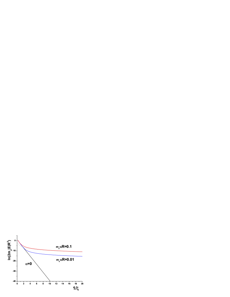
Figure 1: The behavior of the s-level versus the well depth. The curves demonstrate the transition between 2D and 1D regimes. At $\alpha=0$ we have an exponentially shallow level (2D result), while for finite $\alpha$ at small enough $\xi\equiv 2m_{e}U_{0}R^{2}$ the binding energy parabolically depends on $U_{0}$ (1D regime). The dotted line represents the results of our ”pole” approximation (Eq.(Bound states in a 2D short range potential induced by spin-orbit interaction))

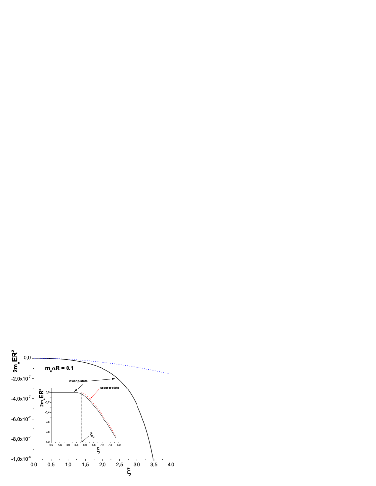
Figure 2: $p$-states. Comparison of the exact solution for the square well with Eq.(Bound states in a 2D short range potential induced by spin-orbit interaction) (dotted line). Inset: spin split states of the $p$-level: the upper curve terminates at $U_{0}=U_{0}^{(c)}$ - the level merges with continuum.

Our last remark relates to the Coulomb interaction with a charged impurity. If one tries to apply the general relation (Bound states in a 2D short range potential induced by spin-orbit interaction) to the Coulomb potential $-e^{2}/r$ the integral logarithmically diverges at the upper limit: $J_{m}^{2}(z\to\infty)\sim(2/\pi z)\cos^{2}{(z-\pi m/4-\pi/4)}$ does not depend on $m$ after averaging over oscillations and can be replaced by $1/\pi z$. Eq.(Bound states in a 2D short range potential induced by spin-orbit interaction) gives for the energy the value independent of $m$:

$$E=-2m_{e}e^{4}\ln^{2}{(p_{0}L)},$$ (23)

where $L$ is some cut-off length. Its exact value depends on the concrete situations: it may be the screening radius or the thickness of 2DEG. We see that the energy spectrum does not depend on $m$ (as it must be for the Coulomb field) and exactly coincides with that of a ”1D hydrogen atom”: the ground state binding energy equals $2Ry$ (rather than $Ry/2$ as in 3D case) multiplied $\ln^{2}(\Lambda)$, where $\Lambda$ is the cut-off parameter (see, for example, the problem of the hydrogen atom in an extremely high magnetic field landau ). This result also supports our interpretation: in the region $|E|\ll m_{e}\alpha^{2}$ the particle becomes effectively one-dimensional.

It is interesting from the general physics point of view to find a similar situation for 3D case. E.G.Batyev has kindly reminded us that the roton spectrum of liquid He-4 also contains a part of dispersion relation that reads $\Delta+(p-p_{0})^{2}/2M$, possesses not a loop but a surface of extrema, and, correspondingly, should describe an effectively 1D particle. We have made the proper calculation, in other words we solved the Schrodinger equation in the momentum representation for the Hamiltonian $\Delta+(p-p_{0})^{2}/2M+U(r)$ with $U(r)$ as an attractive spherically symmetric potential. We used the same method - expansion of the wave function over the spherical harmonics and we got the same result: even in 3D a shallow potential well contains one bound state for each moment $l$ and this state is $(2l+1)$-fold degenerate:

$$E=-2\pi^{2}p_{0}^{2}M\left(\int_{0}^{\infty}dr~{}rU(r)J_{l+1/2}^{2}(p_{0}r)\right)^{2}.$$ (24)

For the Coulomb potential the last formula once again leads to the 1D result given by Eq.(23).

In conclusion, we have shown that 2D electrons interact with impurities by a very special way if one takes into account SO coupling: due to the loop of extrema the system behaves as 1D one for negative energies close to the bottom of continuum. This results in the infinite number of bound states even for a short range potential.

References

• (1) Yu.A.Bychkov and E.I.Rashba, JETP Lett. 39, 78(1984). It is easy to show that Dresswelhaus form of the SO interaction leads to the same results.
• (2) H.Beitman and A.Erdélyi, Higher Transcendential Functions, vol.2 (Mc Graw-Hill book company, Inc., 1953).
• (3) E.I.Rashba and V.I.Sheka, in Landau Level Spectroscopy, ed. by G.Landwehr and E.I.Rashba (Elsevier, 1991), p.178.
• (4) For $s$-level such a transition to 1D regime has been mentioned by A.G.Galstyan and M.E.Raikh (Phys.Rev.B, 58, 6736 (1998)).
• (5) L.D.Landau and E.M.Lifshits, Qvantum Mechanics, (Pergamon Press, Oxford, N.Y., 3rd edn., §112, 1977).