High-order correlation effects in the two-dimensional Hubbard model

Abstract

The electronic states of the two-dimensional Hubbard model are investigated by means of a 4-pole approximation within the Composite Operator Method. In addition to the conventional Hubbard operators, we consider other two operators which come from the hierarchy of the equations of motion and carry information regarding nearest-neighbor spin and charge configurations. By means of this operatorial basis, we can study the physics related to the energy scale of $J=4t^{2}/U$ in addition to the one of $U$. Present results show relevant physical features, well beyond those previously obtained by means of a 2-pole approximation, such as a four-band structure with shadow bands and a quasi-particle peak at the Fermi level. The Fermi level stays pinned to the band flatness located at ($\pi$,$0$)-point within a wide range of hole-doping ($0\leq\delta\leq 0.15$). A comprehensive analysis of double occupancy, internal energy, specific heat and entropy features have been also performed. All reported results are in excellent agreement with the data of numerical simulations.

I Introduction

The discovery of high-$T_{c}$ superconductors promoted a largely diffused revival of interest in strongly correlated electron systems and fostered the study of many other transition-metal oxides.Imada et al. (1998) Since the very beginning, the Hubbard model Hub has received particular attention as it is retained a prototype for strongly correlated electron systems and a minimal model to describe transition-metal oxides. In spite of the deceiving simplicity of its Hamiltonian, a deep comprehension of all its physical features is still missing. In particular, it is very difficult to properly describe the competition between kinetic, diagonal in momentum space, and potential, diagonal in direct space, energy terms. The main gross feature of the model is the splitting of the electronic band into two subbands divided by a gap of the order $U$. Nowadays, it is well-established that this feature can be understood in terms of well-known Hubbard operators within a 2-pole approximation. However, within this framework, inter-site correlations are poorly taken into account while they are universally recognized as essential to describe low-energy physics near half filling. For instance, Kampf and Schrieffer pointed out that, in highly correlated electron systems, antiferromagnetic spin fluctuations play a fundamental role in understanding features as pseudogap and shadow bands.Kampf and Schrieffer (1990a, b) Recently, the remarkable progress in experimental techniques has made possible to reveal such low-energy features in high-$T_{c}$ superconductors.Damascelli et al. (2003) Antiferromagnetic fluctuations are often included within self-energy in a phenomenological way. Therefore, it is quite natural to wonder if, being these features inherent to the model Hamiltonian, it is possible to derive them microscopically by means of a suitable analytical tool. Numerical-simulation techniques, as Exact Diagonalization and quantum Monte Carlo (QMC), positively answer to this question,Dagotto (1994); Bulut et al. (1994); Preuss et al. (1995, 1997) although they are applicable only to small clusters due to the exponential increase of the Hilbert space with the system size. Within the framework of projection methods, in order to describe inter-site correlations and related spin and charge fluctuations, it is necessary to take into account high-order operators which carry information regarding nearest-neighbor correlations. We will move along this way.

In this paper, we investigate the electronic states of the Hubbard model by means of the Composite Operator Method (COM) Ishihara et al. (1994); Mancini et al. (1995a, b); Mancini and Avella (2003, 2004) which has shown to be capable of describing the physics of many strongly correlated systems. On one hand, we can find many similarities between COM and the projection operator method Mori (1965); Roth (1969a, b); Becker et al. (1990); Unger and Fulde (1993); Fulde (1995); Zhou et al. (1991); Mehlig et al. (1995) and the spectral density approach (self-consistent moment approach).Nolting (1972); Geipel and Nolting (1988); Nolting and Borgiel (1989); Rodríguez-Núñez and Argollo de Menezes (1998); Rodríguez-Núñez and Schafroth (1998) On the other hand, COM differs from these methods as regards the conscious exploitation of the presence of unknown parameters in the theory in order to put constraints on the representation where the Green’s functions are realized. The Hubbard model has been widely analyzed by means of COM within the 2-pole approximation.Mancini et al. (1995a, b); Mancini and Avella (2004) In this approximation, COM reaches a global agreement with numerical simulations regarding local and thermodynamic quantities. In order to go beyond the 2-pole approximation, it is necessary either to evaluate the dynamical corrections or to introduce high-order operators in the basis. As regards the former case, a fully momentum and frequency dependent self-energy has been evaluated by means of: two-site level operators within the non-crossing approximation,Matsumoto et al. (1996a, b); Matsumoto and Mancini (1997) loop decoupling within both the self-consistent Born approximation Plakida and Oudovenko (1999); Prelovsek and Ramsak (2002); Krivenko et al. (2005) and the iterative perturbation theory within the dynamical mean field theory.Onoda and Imada (2003) As regards the latter case, Dorneich et al. have introduced in the operatorial basis, in addition to the conventional Hubbard operators, two nonlocal composite fields which describe the local electronic transitions dressed by the nearest-neighbor spin and charge fluctuations.Dorneich et al. (2000) They have managed to reproduce the well-known four band structure in good agreement with the QMC data, but only at half filling to which their formulation is unfortunately restricted. According to all this, we have decided to examine the model by means of a 4-pole approximation within the Composite Operator Method. In addition to the conventional Hubbard operators, we have also considered in the basis other two operators coming from the hierarchy of the equations of motion. Within our formulation, we can evaluate the evolution of each subband up to the second order in the equations of motion and we have managed to perform the analysis with finite doping, which was out of the scope in Ref. Dorneich et al., 2000. Our results present: a four-band structure, a quasi-particle peak at the Fermi level, shadow bands, band flatness at ($\pi$, $0$)-point, a Fermi level located around the ($\pi$, $0$)-point and robust with respect to the hole doping ($\delta\leq 0.15$). A comprehensive study, and comparisons with numerical simulations present in the literature, has been performed as regards: density of states, band dispersion, double occupancy, internal energy, specific heat and entropy.

The manuscript is organized as follows. In the next section (Sec. II), we fix the notation regarding the Hamiltonian and give the general framework of the Composite Operator Method. In Sec. III, the density of states and the dispersion relation are computed and discussed, also in comparison with some quantum Monte Carlo results. A detailed comparison with numerical simulations for many local and thermodynamic quantities is given in Sec. IV. Section V contains summary and conclusions. Some detailed derivations of formulas used in Sec. III are given in the appendix.

II Model and Formulation

The two-dimensional grand-canonical Hubbard Hamiltonian $\hat{H}$ reads as

$$\hat{H} =H-\mu\sum_{\mathbf{i}\sigma}n_{\sigma}(i)$$ (1)

$$H =\sum_{\mathbf{ij}\sigma}t_{\mathbf{ij}}c^{\dagger}_{\sigma}(i)c_{\sigma}(j)+U\sum_{\mathbf{i}}n_{\uparrow}(i)n_{\downarrow}(i)$$ (2)

where $c^{\dagger}_{\sigma}(i)$ and $c_{\sigma}(i)$ are creation and annihilation operators, respectively, of electrons with spin $\sigma$ at the site $\mathbf{i}$ $[i=(\mathbf{i},t)]$. $n_{\sigma}(i)=c^{\dagger}_{\sigma}(i)c_{\sigma}(i)$. $\mu$ is the chemical potential. $t_{\mathbf{ij}}=-4t\alpha_{\mathbf{ij}}$. $\alpha(\mathbf{k})=\mathcal{F}[\alpha_{\mathbf{ij}}]=\frac{1}{2}\left\{\cos(k_{x}a)+\cos(k_{y}a)\right\}$. $a$ is the lattice constant. $\mathcal{F}$ is the Fourier transform. $U$ is the on-site Coulomb repulsion. Here, we consider nearest-neighbor hopping only. We define the following operatorial basis

$$\psi_{\sigma}(i)=\left(\begin{array}[]{c}\psi_{A\sigma}(i)\\ \psi_{B\sigma}(i)\end{array}\right)=\left(\begin{array}[]{c}\xi_{\sigma}(i)\\ \eta_{\sigma}(i)\\ \hline\cr\xi_{s\sigma}(i)\\ \eta_{s\sigma}(i)\end{array}\right)$$ (3)

where $\xi_{\sigma}(i)=\left(1-n_{-\sigma}(i)\right)c_{\sigma}(i)$ and $\eta_{\sigma}(i)=n_{-\sigma}(i)c_{\sigma}(i)$ are the usual Hubbard operators that describe the transitions of the local electron number $n(i)=0\leftrightarrow 1$ and $1\leftrightarrow 2$, respectively. The equations of motion of the components of $\psi_{A}(i)$ read as

$$\mathrm{i}\frac{\partial}{\partial t}\xi_{\sigma}(i)=-\mu\xi_{\sigma}(i)-4t\left\{c^{\alpha}_{\sigma}(i)+\pi_{\sigma}(i)\right\}$$ (4)

$$\mathrm{i}\frac{\partial}{\partial t}\eta_{\sigma}(i)=(-\mu+U)\eta_{\sigma}(i)+4t\pi_{\sigma}(i)$$ (5)

where

$$\pi_{\sigma}(i) =-n_{-\sigma}(i)c^{\alpha}_{\sigma}(i)+c^{\dagger}_{-\sigma}(i)c_{\sigma}(i)c^{\alpha}_{-\sigma}(i)$$

$$+c_{\sigma}(i)c^{\alpha\dagger}_{-\sigma}(i)c_{-\sigma}(i)$$ (6)

$$c^{\alpha}_{\sigma}(i) =\sum_{\bf j}\alpha_{\bf ij}c_{\sigma}({\bf j},t).$$ (7)

Now, we can divide $\pi_{\sigma}(i)$ into two operators, $\pi_{\sigma}(i)=\xi_{s\sigma}(i)+\eta_{s\sigma}(i)$, similarly to what we have done with $c_{\sigma}(i)$, $c_{\sigma}(i)=\xi_{\sigma}(i)+\eta_{\sigma}(i)$. That is, we choose the components of $\psi_{B}(i)$, $\xi_{s\sigma}(i)$ and $\eta_{s\sigma}(i)$, among the eigenoperators of the two-site Hubbard model Avella et al. (2003) and of the local interaction term of the Hamiltonian (1). Then, they read as

$$\xi_{s\sigma}(i) =-n_{-\sigma}(i)\xi^{\alpha}_{\sigma}(i)$$

$$+c^{\dagger}_{-\sigma}(i)c_{\sigma}(i)\xi^{\alpha}_{-\sigma}(i)+c_{\sigma}(i)\eta^{\alpha\dagger}_{-\sigma}(i)c_{-\sigma}(i)$$ (8)

$$\eta_{s\sigma}(i) =-n_{-\sigma}(i)\eta^{\alpha}_{\sigma}(i)$$

$$+c^{\dagger}_{-\sigma}(i)c_{\sigma}(i)\eta^{\alpha}_{-\sigma}(i)+c_{\sigma}(i)\xi^{\alpha\dagger}_{-\sigma}(i)c_{-\sigma}(i).$$ (9)

It is clear now that $\psi_{B}(i)$ describes nearest-neighbor composite excitations and carries information regarding surrounding spin and charge configurations.Odashima et al. (2005) According to the way we have chosen them,Avella et al. (2003) $\xi_{\sigma}(i)$ and $\xi_{s\sigma}(i)$ belong to the energy class of the lower Hubbard subband and $\eta_{\sigma}(i)$ and $\eta_{s\sigma}(i)$ belong to the energy class of the upper Hubbard subband (see Eqs. (4), (5), (73) and (74)).

Within the Composite Operator Method, once we choose a $n$-component operatorial basis $\psi$, its equation of motion reads as

$$\mathrm{i}\frac{\partial}{\partial t}\psi(i)=\sum_{\bf j}\epsilon({\bf i},{\bf j})\psi({\bf j},t)+\delta j(i)$$ (10)

where $\epsilon({\bf k})=m({\bf k})I^{-1}({\bf k})$ is a $n\times n$ matrix with

$$I({\bf k})=\mathcal{F}\langle\{\psi({\bf i},t),\psi^{\dagger}({\bf j},t)\}\rangle$$ (11)

$$m({\bf k})=\mathcal{F}\langle\{i\frac{\partial}{\partial t}\psi({\bf i},t),\psi^{\dagger}({\bf j},t)\}\rangle.$$ (12)

The spinor notation is understood and $\langle\cdots\rangle$ denotes the thermal average in the grand-canonical ensemble. The expression of $\epsilon({\bf k})$ comes from the request $\langle\{\delta j({\bf i},t),\psi^{\dagger}({\bf j},t)\}\rangle=0$. This constraint assures that the residual term $\delta j(i)$ contains only the dynamical corrections in terms of orthogonal components to the chosen basis. Neglecting $\delta j(i)$ gives the $n$-pole approximation for the retarded electronic Green’s function $G(\omega,{\bf k})=\mathcal{F}\left\langle R[\psi(i)\psi^{\dagger}(j)]\right\rangle$:

$$G(\omega,{\bf k})=\sum_{i=1}^{n}\frac{\sigma_{i}({\bf k})}{\omega-E_{i}({\bf k})+\mathrm{i}\delta}$$ (13)

where $E_{i}({\bf k})$ are the eigenvalues of $\epsilon({\bf k})$ and $\sigma_{i}({\bf k})$, the spectral functions, can be computed in terms of the eigenvectors of $\epsilon({\bf k})$ and of the elements of $I({\bf k})$.Mancini and Avella (2003, 2004)

In the last years, the 2-pole approximation, that is, $\psi=\psi_{A}$, has been analyzed in great detail.Mancini and Avella (2004) In the present paper, we perform a 4-pole analysis by enlarging the operatorial basis with the introduction of $\psi_{B}$. In this case, $I({\bf k})$ reads as

$$I({\bf k}) =\left(\begin{array}[]{cc}I_{AA}({\bf k})&I_{AB}({\bf k})\\ I_{AB}({\bf k})&I_{BB}({\bf k})\end{array}\right)$$ (16)

$$=\left(\begin{array}[]{cc|cc}I_{11}&0&I_{13}({\bf k})&0\\ 0&I_{22}&0&I_{24}({\bf k})\\ \hline\cr I_{13}({\bf k})&0&I_{33}({\bf k})&I_{34}({\bf k})\\ 0&I_{24}({\bf k})&I_{34}({\bf k})&I_{44}({\bf k})\end{array}\right)$$ (21)

where

$$I_{11\sigma}=1-\langle n_{-\sigma}\rangle$$ (22)

$$I_{22\sigma}=\langle n_{-\sigma}\rangle$$ (23)

$$I_{13\sigma}({\bf k})=\Delta_{\sigma}-\alpha({\bf k})\left(\langle n_{-\sigma}\rangle-p_{\sigma}\right)$$ (24)

$$I_{24\sigma}({\bf k})=-\Delta_{\sigma}-\alpha({\bf k})p_{\sigma}$$ (25)

with

$$\Delta_{\sigma} =\langle\eta^{\dagger}_{-\sigma}\eta^{\alpha}_{-\sigma}\rangle-\langle\xi^{\dagger}_{-\sigma}\xi^{\alpha}_{-\sigma}\rangle$$ (26)

$$p_{\sigma} =\langle n_{-\sigma}n^{\alpha}_{-\sigma}\rangle+\langle c^{\dagger}_{-\sigma}c_{\sigma}(c^{\dagger}_{\sigma}c_{-\sigma})^{\alpha}\rangle$$

$$-\langle c_{\sigma}c_{-\sigma}(c^{\dagger}_{-\sigma}c^{\dagger}_{\sigma})^{\alpha}\rangle.$$ (27)

The detailed expressions of the elements in the block $I_{BB}({\bf k})$ are rather complicated and reported in Appendix. In order to effectively perform calculations, we have decoupled these elements by paying attention to the particle-hole symmetry enjoined by the Hamiltonian. Under this transformation, we have

$$\xi_{\sigma}(i)\rightarrow(-1)^{\bf i}\eta^{\dagger}_{\sigma}(i)$$ (28)

$$\eta_{\sigma}(i)\rightarrow(-1)^{\bf i}\xi^{\dagger}_{\sigma}(i)$$ (29)

$$\xi_{s\sigma}(i)\rightarrow(-1)^{\bf i}\eta^{\alpha\dagger}_{\sigma}(i)+(-1)^{\bf i}\eta^{\dagger}_{s\sigma}(i)$$ (30)

$$\eta_{s\sigma}(i)\rightarrow(-1)^{\bf i}\xi^{\alpha\dagger}_{\sigma}(i)+(-1)^{\bf i}\xi^{\dagger}_{s\sigma}(i).$$ (31)

After these relations, we have the following constraints on the $I_{\sigma}({\bf i,j})=\langle\{\psi_{\sigma}({\bf i},t),\psi^{\dagger}_{\sigma}({\bf j},t)\}\rangle$ matrix elements

$$I_{11}({\bf i,j})\rightarrow (-1)^{\bf i+j}I_{22}({\bf j,i})$$ (32)

$$I_{22}({\bf i,j})\rightarrow (-1)^{\bf i+j}I_{11}({\bf j,i})$$ (33)

$$I_{33}({\bf i,j})\rightarrow (-1)^{\bf i+j}\{I_{22}({\bf j^{\alpha},i^{\alpha}})+I_{24}({\bf j^{\alpha},i})\}$$

$$+ (-1)^{\bf i+j}\{I_{42}({\bf j,i^{\alpha}})+I_{44}({\bf j,i})\}$$ (34)

$$I_{34}({\bf i,j})\rightarrow (-1)^{\bf i+j}I_{34}({\bf j,i})$$ (35)

$$I_{44}({\bf i,j})\rightarrow (-1)^{\bf i+j}\{I_{11}({\bf j^{\alpha},i^{\alpha}})+I_{13}({\bf j^{\alpha},i})\}$$

$$+ (-1)^{\bf i+j}\{I_{31}({\bf j,i^{\alpha}})+I_{33}({\bf j,i})\}$$ (36)

where ${\bf i}^{\alpha}$ stands for the nearest-neighbor sites of $\bf i$ (e.g., $I_{13}({\bf j^{\alpha},i})=\sum_{\bf l}\alpha_{\bf jl}I_{13}({\bf l,i})$). It is worth noticing that our decoupling procedure exactly satisfies these relations.

Now, we introduce a new operator

$$\bar{\psi}_{B\sigma}(i)=\left(\begin{array}[]{c}\bar{\xi}_{s\sigma}(i)\\ \bar{\eta}_{s\sigma}(i)\end{array}\right)=\left(\begin{array}[]{c}\xi_{s\sigma}(i)-A_{31}(-\mathrm{i}\nabla)\xi_{\sigma}(i)\\ \eta_{s\sigma}(i)-A_{42}(-\mathrm{i}\nabla)\eta_{\sigma}(i)\end{array}\right)$$ (37)

with

$$\mathcal{F}\left[A_{31}(-\mathrm{i}\nabla)\right]=A_{31}({\bf k})=\frac{I_{13}({\bf k})}{I_{11}}$$ (38)

$$\mathcal{F}\left[A_{42}(-\mathrm{i}\nabla)\right]=A_{42}({\bf k})=\frac{I_{24}({\bf k})}{I_{22}}.$$ (39)

This operator gives $I$ in a block-diagonal form

$$I({\bf k}) =\left(\begin{array}[]{cc}I_{AA}({\bf k})&0\\ 0&I_{BB}({\bf k})\end{array}\right)$$ (42)

$$=\left(\begin{array}[]{cc|cc}I_{11}&0&0&0\\ 0&I_{22}&0&0\\ \hline\cr 0&0&\bar{I}_{33}({\bf k})&\bar{I}_{34}({\bf k})\\ 0&0&\bar{I}_{34}({\bf k})&\bar{I}_{44}({\bf k})\end{array}\right)$$ (47)

where

$$\bar{I}_{33}({\bf k})=I_{33}({\bf k})-\frac{I^{2}_{13}({\bf k})}{I_{11}}$$ (48)

$$\bar{I}_{34}({\bf k})=I_{34}({\bf k})$$ (49)

$$\bar{I}_{44}({\bf k})=I_{44}({\bf k})-\frac{I^{2}_{24}({\bf k})}{I_{22}}.$$ (50)

Hereafter, we will use this new operator $\bar{\psi}_{B\sigma}(i)$ instead of $\psi_{B\sigma}(i)$ as it allows to more easily distinguish the contributions to single-particle properties of type $B$ operators from those of type $A$. Then

$$\psi_{\sigma}(i)=\left(\begin{array}[]{c}\psi_{A\sigma}(i)\\ \bar{\psi}_{B\sigma}(i)\end{array}\right).$$ (51)

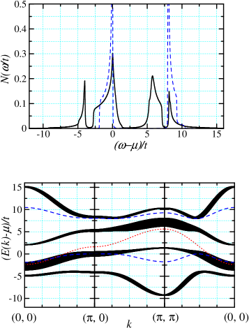
Figure 1: The density of states and the corresponding dispersion relation (solid line) at $U/t=8$, $n=0.90$ and $T/t=0.01$. The width of the dispersion line represents the intensity of peak. The 2-pole solution (dashed line) and the non-interacting case (dotted line) are also reported.

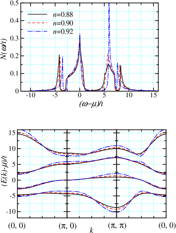
Figure 2: Doping dependence of density of states and dispersion relation at $n=0.88$, $0.90$ and $0.92$. Other external parameters are the same as in Fig. 1.

By means of this new basis, we have the matrix $\epsilon=mI^{-1}$,

$$\epsilon({\bf k}) =\left(\begin{array}[]{cc}\epsilon_{AA}({\bf k})&\epsilon_{AB}({\bf k})\\ \epsilon_{BA}({\bf k})&\epsilon_{BB}({\bf k})\end{array}\right)$$ (54)

$$=\left(\begin{array}[]{cc|cc}\epsilon_{11}({\bf k})&\epsilon_{12}({\bf k})&\epsilon_{13}({\bf k})&\epsilon_{14}({\bf k})\\ \epsilon_{21}({\bf k})&\epsilon_{22}({\bf k})&\epsilon_{23}({\bf k})&\epsilon_{24}({\bf k})\\ \hline\cr\epsilon_{31}({\bf k})&\epsilon_{32}({\bf k})&\epsilon_{33}({\bf k})&\epsilon_{34}({\bf k})\\ \epsilon_{41}({\bf k})&\epsilon_{42}({\bf k})&\epsilon_{43}({\bf k})&\epsilon_{44}({\bf k})\end{array}\right)$$ (59)

where

$$\epsilon_{11}({\bf k})=-\mu-4t\left(\alpha({\bf k})+\frac{I_{13}({\bf k})}{I_{11}}\right)$$ (60)

$$\epsilon_{12}({\bf k})=-4t\left(\alpha({\bf k})+\frac{I_{24}({\bf k})}{I_{22}}\right)$$ (61)

$$\epsilon_{21}({\bf k})=4t\frac{I_{13}({\bf k})}{I_{11}}$$ (62)

$$\epsilon_{22}({\bf k})=-\mu+U+4t\frac{I_{24}({\bf k})}{I_{22}}$$ (63)

$$\epsilon_{13}({\bf k})=\epsilon_{14}({\bf k})=-\epsilon_{23}({\bf k})=-\epsilon_{24}({\bf k})=-4t$$ (64)

$$\epsilon_{31}({\bf k})=-4t\frac{\bar{I}_{33}({\bf k})+\bar{I}_{34}({\bf k})}{I_{11}}$$ (65)

$$\epsilon_{32}({\bf k})=4t\frac{\bar{I}_{33}({\bf k})+\bar{I}_{34}({\bf k})}{I_{22}}$$ (66)

$$\epsilon_{41}({\bf k})=-4t\frac{\bar{I}_{43}({\bf k})+\bar{I}_{44}({\bf k})}{I_{11}}$$ (67)

$$\epsilon_{42}({\bf k})=4t\frac{\bar{I}_{43}({\bf k})+\bar{I}_{44}({\bf k})}{I_{22}}$$ (68)

and

$$\epsilon_{BB}({\bf k})=m_{BB}({\bf k})I^{-1}_{BB}({\bf k})$$ (69)

where

$$m_{BB}({\bf k}) =\mathcal{F}\langle\{i\frac{\partial}{\partial t}\bar{\psi}_{B\sigma}({\bf i},t),\bar{\psi}^{\dagger}_{B\sigma}({\bf j},t)\}\rangle$$

$$=\left(\begin{array}[]{cc}m_{33}({\bf k})&m_{34}({\bf k})\\ m_{34}({\bf k})&m_{44}({\bf k})\end{array}\right).$$ (72)

The operator $\bar{\psi}_{B\sigma}(i)$ provides two-site excitations and represents the natural extension of $\psi_{A\sigma}(i)$, which describes one-site excitations, in the sense of a series expansion over finite-cluster excitations. Equations of motion of $\bar{\psi}_{B\sigma}(i)$ are much more lengthy and have a much more complex form with respect to those of $\psi_{A\sigma}(i)$ as they contain many three-site composite operators. The application of a systematic projection/truncation procedure, as the one applied to the equations of motion of $\psi_{A\sigma}(i)$, is just unfeasible in this case as, besides to be very lengthy, it would lead to the appearance of a plenty of unknown correlation functions in the energy matrix. In order to fix all these correlation functions, we would be forced to use some decoupling and would completely lose any possibility to control the approximation. Then, we have opted for a controlled, at least in philosophy, approximation at the level of equations of motion and decided to neglect irreducible three-site operators by paying attention to evaluate exactly all one- and two-site components Odashima et al. (2005). This choice has only one obvious drawback: the two-site correlations, not damped by three-site processes, result quite enhanced.

$$\mathrm{i}\frac{\partial}{\partial t}\xi_{s\sigma}(i)\simeq-\mu\xi_{s\sigma}(i)+4t\left\{\frac{1}{2}\eta_{\sigma}(i)+\xi^{\alpha}_{s\sigma}(i)+2\eta^{\alpha}_{s\sigma}(i)\right\}$$ (73)

$$\mathrm{i}\frac{\partial}{\partial t}\eta_{s\sigma}(i)\simeq(-\mu+U)\eta_{s\sigma}(i)+4t\left\{\frac{1}{4}\eta_{\sigma}(i)+\xi^{\alpha}_{s\sigma}(i)\right\}.$$ (74)

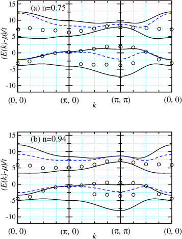
Figure 3: The dispersion relation at $U/t=8$, $T/t=0.5$ and $n=0.75$ and $0.94$. The 2-pole solution (dashed line) and QMC data (circle) of Ref. Bulut et al., 1994 are also reported.

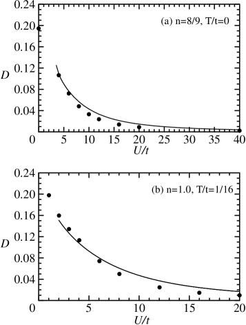
Figure 4: Double occupancy (solid line) versus $U/t$ at (a) $n=8/9$ and $T/t=0$ (Lanczos data (circle) from Ref. Becca et al., 2000) and (b) $n=1.0$ and $T/t=1/16$ (QMC data (circle) from Ref. White et al., 1989).

Equations of motion (73) and (74) give a simplified form of $\epsilon_{BB}({\bf k})$

$$\epsilon_{33}({\bf k})=-\mu+4t\left(\alpha({\bf k})+\frac{I_{13}({\bf k})}{I_{11}}\right)$$ (75)

$$\epsilon_{34}({\bf k})=4t\left(2\alpha({\bf k})+\frac{I_{13}({\bf k})}{I_{11}}\right)$$ (76)

$$\epsilon_{43}({\bf k})=4t\left(\alpha({\bf k})-\frac{I_{24}({\bf k})}{I_{22}}\right)$$ (77)

$$\epsilon_{44}({\bf k})=-\mu+U-4t\frac{I_{24}({\bf k})}{I_{22}}.$$ (78)

The correlation functions appearing in $I$ and $\epsilon$, except for $p_{\sigma}$, can be now self-consistently determined through the retarded Green’s function

$$\langle\psi\psi^{\dagger}\rangle=\left(\frac{a}{2\pi}\right)^{2}\iint d{\bf k}\,d\omega\,\left[1-f_{F}(\omega)\right]\left(-\frac{1}{\pi}\Im\left[G(\omega,{\bf k})\right]\right)$$ (79)

where $f_{F}(\omega)$ is the Fermi distribution function.

The parameters $p_{\sigma}$ are out of the scheme of the present formulation as they cannot be directly connected to the Green’s function under study. They describe nearest-neighbor spin, charge and pair correlations and, according to their actual values, play a fundamental role in determining the behavior of the system (antiferromagnetic character of the band dispersion, presence of metal-insulator transition, etc.).Mancini and Avella (2004) The use of operators not satisfying canonical commutation relations leads to the appearance of unknown correlation functions in the formulation. The presence of these unknown correlation function should not be seen as an inconvenience, as many other formulations do, but as an opportunity given by the method to implement exact relations dictated by symmetries and/or general principles which are not automatically satisfied, that is, which are no more embedded in the Hilbert space of the composite operators whose Green’s functions are computed.Mancini and Avella (2003, 2004) According to this, we will evaluate $p_{\sigma}$ by means of the algebra constraints Mancini and Avella (2003, 2004) $\langle\xi^{\dagger}_{\sigma}\eta_{\sigma}\rangle=0$. These constraints ensure that no state referring to a triple-occupied site (obviously forbidden by the Pauli principle) is taken into account in the averaging procedure and give the possibility to make the correct spin/particle counting. This allows to fulfil the particle-hole symmetry and to correctly describe the virtual processes at the basis of the low-energy processes ($J$ scale of energy). A comprehensive analysis by means of the two-pole approximation has shown that the use of algebraic constraints provides very good agreement with the numerical simulation results well beyond the conventional Hubbard-I and Roth’s decoupling scheme. Mancini and Avella (2004)

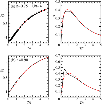
Figure 5: Internal energy and specific heat at $U/t=4$ and $n=0.75$ and $0.90$ (solid line). Finite temperature Lanczos data (dashed line) from Ref. Bonc̆a and Prelovšek, 2003 and QMC data (circle) from Ref. Duffy and Moreo, 1997 are also reported.

III BAND STRUCTURE

Figure 1 shows the density of states and the corresponding dispersion relation for $U/t=8$, $n=0.9$ and $T/t=0.01$. As a first consequence of choosing a basis constituted of four operators, we have a four-band structure. Together with the usual Hubbard splitting of the non-interacting band with the appearance of a gap of the order $U$ between the Hubbard subbands, we can clearly observe other two dispersion lines in the lower and higher energy regions ($\omega/t\sim-4$ and $8$). They can be interpreted as shadow bands coming from the antiferromagnetic nature of the spin fluctuations. In fact, they show a tendency towards a doubling of the zone through a mirroring of the original dispersion lines. Another remarkable feature is the presence of a well developed peak structure at the Fermi level which comes from the band flatness around the ($\pi$,$0$)-point. Some peculiar features of the 2-pole solution (e.g., the inflexion around the ($\pi$,$\pi$)-point) can be now clearly interpreted as due to the necessity of miming the behavior of both Hubbard subbands and shadow bands by means of only two bands.

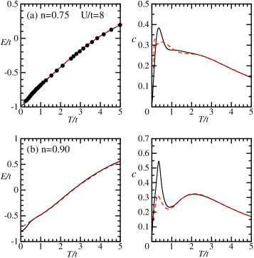
Figure 6: Same of Fig. 5 but at $U/t=8$.

In Fig. 2, we present the doping dependence of the density of states and of the corresponding dispersion relation. The Fermi level stays pinned to the band flatness located at ($\pi$,$0$)-point within a wide range of hole-doping ($0\leq\delta\leq 0.15$). For higher doping, it moves towards higher energies giving an electron-like Fermi surface centered at ($0$,$0$)-point. Those characteristics are commonly observed in many theoretical analysis Matsumoto et al. (1996a); Matsumoto and Mancini (1997); Krivenko et al. (2005); Onoda and Imada (2003); Dorneich et al. (2000); Odashima et al. (2005) which take into account nearest-neighbor spin and charge fluctuations, in agreement with QMC data.Bulut et al. (1994); Preuss et al. (1995, 1997) Therefore, we can conclude that in order to reproduce such peculiar features, it is necessary to take into account high-order operators in the basis, as we have done in this manuscript.

In Fig. 3, we provide a detailed comparison of the band structure obtained by the present formulation with QMC results. As can be easily seen, we have a good agreement with QMC data, especially for the low-energy band around the Fermi level. We observe shadow bands more pronounced than in QMC data. We should recall that the present formulation is a pole-approximation and damping effects are neglected. Furthermore, three-site terms in the equations of motion have been neglected. Therefore, there is no diffusion process to weaken two-site correlation effects. On the other hand, we can expect that with hole-doping the antiferromagnetic correlations are weakened by hole motion and that the shadow bands become broader and broader owing to damping effects. Eventually, shadow bands are wiped out and we may observe traces of them as shoulders of the main Hubbard bands, as seen in QMC results.

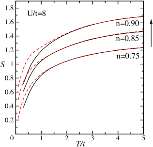
Figure 7: Entropy at $U/t=8$ (solid line) (Finite temperature Lanczos data (dashed line) from Ref. Bonc̆a and Prelovšek, 2003). Data are shifted of $0.2$ along the vertical axis for the sake of clarity.

IV THERMODYNAMIC QUANTITIES

Figure 4 presents double occupancy $D=\langle n_{\uparrow}n_{\downarrow}\rangle=\langle\eta^{\dagger}_{\sigma}\eta_{\sigma}\rangle$ in comparison with Lanczos Becca et al. (2000) and QMC White et al. (1989) results. For $U/t<3$, it is difficult to get self-consistent solution as split bands start merging. Our results show a good agreement in a wide range of $U/t$ values. We should point out that the 2-pole approximation also provides similar agreement.Mancini and Avella (2004)

Internal energy $E=\langle H\rangle/N$ and specific heat $C=dE/dT$ per site at $U/t=4$ and $8$ and $n=0.75$ and $0.90$ are reported in Figs. 5 and 6. Data from finite temperature Lanczos Bonc̆a and Prelovšek (2003) and QMC Duffy and Moreo (1997) are provided for comparison. It is worth mentioning that our results for $U/t=12$ have the same general features that those for $U/t=8$, but with more pronounced characteristics. As regards the internal energy, the agreement with the Lanczos data is excellent except for the low temperature region $T/t<0.4$ at $U/t\geq 8$. As regards the specific heat, we observe a sharp peak around $T/t\sim 0.3$ and a fairly broad peak in the higher temperature region $T/t>1$. The two peak structure is more pronounced for $U/t\geq 8$, but not so much for $U/t=4$. This tendency is also observed in several numerical simulations.Bonc̆a and Prelovšek (2003); Duffy and Moreo (1997); Paiva et al. (2001) Usually, the sharp peak at lower temperatures and the broad peak at higher temperatures are interpreted as consequences of spin and charge fluctuations related to the energy scales of $J$ and $U$, respectively. The main difference between our results and numerical ones regards the height of the peak in the specific heat around $T/t\sim 0.3$ that comes from the decrease in the internal energy. This is an indication of well established spin ordering which cannot be correctly evaluated on a small cluster. Numerical simulation cannot describe spin and charge ordering in the case that the correlation lengths exceed the cluster size. On the other hand, in our formulation, as already discussed in Sec. III, there is no diffusion process to weaken two-site correlation effects. Therefore, there is a tendency to have too pronounced spin and charge correlations.

Figure 8: Entropy vs $n$ at $U/t=4$, $8$ and $12$ and $T/t=0.5$, $1.0$ and $3.0$ (lines) (Finite temperature Lanczos data (markers) from Ref. Bonc̆a and Prelovšek, 2003).

We can discuss this issue in more detail by commenting our results on entropy

$$S(T,n)=-\int^{n}_{0}dn^{\prime}\left(\frac{\partial\mu}{\partial T}\right)_{n^{\prime}}.$$ (80)

This relation is derived from the thermodynamic relations Mancini et al. (1999); Mancini and Avella (2004) $S=-\left(\frac{\partial F}{\partial T}\right)_{n}$ and $\mu=\left(\frac{\partial F}{\partial n}\right)_{T}$, which give the Maxwell relation $\left(\frac{\partial S}{\partial n}\right)_{T}=-\left(\frac{\partial\mu}{\partial T}\right)_{n}$. Figure 7 reports the results of entropy in comparison with Lanczos ones. We present results only for $U/t=8$, but $U/t=4$ and $12$ results show the same tendency. Our results completely coincide with Lanczos ones in the high-temperature region ($T/t>1$). In the low-temperature region ($T/t<1$), our data are lower than Lanczos ones indicating a stronger tendency to ordering.

To better understand the tendency to ordering, we have investigated the filling dependence of entropy at several temperatures (see Fig. 8). For $T/t\geq 1.0$, the agreement is extremely good in whole range of filling. However, at lower temperatures, our results show a decrease around both quarter and half filling. Usually, a decrease of entropy at quarter and half filling is interpreted as an indication of charge and spin ordering, respectively. In a small cluster, it is difficult to investigate such ordered states because of the system size.

V SUMMARY

In the present paper, we have carried out an analysis of the two-dimensional Hubbard model by means of a 4-pole approximation within the Composite Operator Method. Density of states and corresponding dispersion relation show remarkable characteristics: four-bands structure, a quasi-particle peak at the Fermi level, shadow bands and band flatness at ($\pi$, $0$)-point. Quantities such as double occupancy, internal energy, specific heat and entropy have been comprehensively investigated. Our results show an excellent agreement with numerical simulations except for the low energy features related to spin and charge ordering. In the present formulation, nearest-neighbor-site effects are probably over-estimated whereas on a small cluster there are some difficulties to describe spin and charge ordering in the case that the correlation length exceeds the system size. Probably the right stays in the middle: our results provide meaningful information for band structure and thermodynamic quantities, but the inclusion of damping effects is necessary for complete understanding of this system.

Appendix A

The equations of motion of $\xi_{s\sigma}(i)$ and $\eta_{s\sigma}(i)$ reads as

$$\begin{array}[]{l}\displaystyle\mathrm{i}\frac{\partial}{\partial t}\xi_{s\sigma}(i)=-\mu\xi_{s\sigma}(i)\\ \displaystyle\hskip 14.22636pt-4t\left\{\begin{array}[]{l}-n_{-\sigma}(i)c^{\alpha^{2}}_{\sigma}(i)+n_{-\sigma}(i)(n_{-\sigma}(i)c^{\alpha}_{\sigma}(i))^{\alpha}-n_{-\sigma}(i)(c^{\dagger}_{-\sigma}(i)c_{\sigma}(i)c^{\alpha}_{-\sigma}(i))^{\alpha}\\ +n_{-\sigma}(i)(c^{\alpha\dagger}_{-\sigma}(i)c_{\sigma}(i)c_{-\sigma}(i))^{\alpha}-c^{\dagger}_{-\sigma}(i)c^{\alpha}_{-\sigma}(i)\xi^{\alpha}_{\sigma}(i)+c^{\alpha\dagger}_{-\sigma}(i)c_{-\sigma}(i)\xi^{\alpha}_{\sigma}(i)\\ +c^{\dagger}_{-\sigma}(i)c_{\sigma}(i)c^{\alpha^{2}}_{-\sigma}(i)-c^{\dagger}_{-\sigma}(i)c_{\sigma}(i)(n_{\sigma}(i)c^{\alpha}_{-\sigma}(i))^{\alpha}+c^{\dagger}_{-\sigma}(i)c_{\sigma}(i)(c^{\dagger}_{\sigma}(i)c_{-\sigma}(i)c^{\alpha}_{\sigma}(i))^{\alpha}\\ -c^{\dagger}_{-\sigma}(i)c_{\sigma}(i)(c^{\alpha\dagger}_{\sigma}(i)c_{-\sigma}(i)c_{\sigma}(i))^{\alpha}+c^{\dagger}_{-\sigma}(i)c^{\alpha}_{\sigma}(i)\xi^{\alpha}_{-\sigma}(i)-c^{\alpha\dagger}_{-\sigma}(i)c_{\sigma}(i)\xi^{\alpha}_{-\sigma}(i)\\ -\eta^{\alpha\dagger}_{-\sigma}(i)c_{\sigma}(i)c^{\alpha}_{-\sigma}(i)-\eta^{\alpha\dagger}_{-\sigma}(i)c^{\alpha}_{\sigma}(i)c_{-\sigma}(i)+(c^{\dagger}_{\sigma}(i)c^{\dagger}_{-\sigma}(i)c^{\alpha}_{\sigma}(i))^{\alpha}c_{\sigma}(i)c_{-\sigma}(i)\\ +(c^{\alpha\dagger}_{-\sigma}(i)n_{\sigma}(i))^{\alpha}c_{\sigma}(i)c_{-\sigma}(i)+(c^{\alpha\dagger}_{\sigma}(i)c_{\sigma}(i)c^{\dagger}_{-\sigma}(i))^{\alpha}c_{\sigma}(i)c_{-\sigma}(i)\end{array}\right\}\end{array}$$ (81)

$$\begin{array}[]{l}\displaystyle\mathrm{i}\frac{\partial}{\partial t}\eta_{s\sigma}(i)=(-\mu+U)\eta_{s\sigma}(i)\\ \displaystyle\hskip 14.22636pt-4t\left\{\begin{array}[]{l}-n_{-\sigma}(i)(n_{-\sigma}(i)c^{\alpha}_{\sigma}(i))^{\alpha}+n_{-\sigma}(i)(c^{\dagger}_{-\sigma}(i)c_{\sigma}(i)c^{\alpha}_{-\sigma}(i))^{\alpha}-n_{-\sigma}(i)(c^{\alpha\dagger}_{-\sigma}(i)c_{\sigma}(i)c_{-\sigma}(i))^{\alpha}\\ -c^{\dagger}_{-\sigma}(i)c^{\alpha}_{-\sigma}(i)\eta^{\alpha}_{\sigma}(i)+c^{\alpha\dagger}_{-\sigma}(i)c_{-\sigma}(i)\eta^{\alpha}_{\sigma}(i)+c^{\dagger}_{-\sigma}(i)c_{\sigma}(i)(n_{\sigma}(i)c^{\alpha}_{-\sigma}(i))^{\alpha}\\ -c^{\dagger}_{-\sigma}(i)c_{\sigma}(i)(c^{\dagger}_{\sigma}(i)c_{-\sigma}(i)c^{\alpha}_{\sigma}(i))^{\alpha}+c^{\dagger}_{-\sigma}(i)c_{\sigma}(i)(c^{\alpha\dagger}_{\sigma}(i)c_{-\sigma}(i)c_{\sigma}(i))^{\alpha}\\ +c^{\dagger}_{-\sigma}(i)c^{\alpha}_{\sigma}(i)\eta^{\alpha}_{-\sigma}(i)-c^{\alpha\dagger}_{-\sigma}(i)c_{\sigma}(i)\eta^{\alpha}_{-\sigma}(i)-\xi^{\alpha\dagger}_{-\sigma}(i)c_{\sigma}(i)c^{\alpha}_{-\sigma}(i)-\xi^{\alpha\dagger}_{-\sigma}(i)c^{\alpha}_{\sigma}(i)c_{-\sigma}(i)\\ -(c^{\dagger}_{\sigma}(i)c^{\dagger}_{-\sigma}(i)c^{\alpha}_{\sigma}(i))^{\alpha}c_{\sigma}(i)c_{-\sigma}(i)+c^{\alpha^{2}\dagger}_{-\sigma}(i)c_{\sigma}(i)c_{-\sigma}(i)-(c^{\alpha\dagger}_{-\sigma}(i)n_{\sigma}(i))^{\alpha}c_{\sigma}(i)c_{-\sigma}(i)\\ -(c^{\alpha\dagger}_{\sigma}(i)c_{\sigma}(i)c^{\dagger}_{-\sigma}(i))^{\alpha}c_{\sigma}(i)c_{-\sigma}(i)\end{array}\right\}\end{array}$$ (82)

where $A^{\alpha^{2}}(i)$ and $A^{\alpha}(i)B^{\alpha}(i)$ stand for

$$A^{\alpha^{2}}(i)=\sum_{\bf j,k}\alpha_{\bf ij}\alpha_{\bf jk}A(k)$$ (83)

and

$$A^{\alpha}(i)B^{\alpha}(i)=\sum_{\bf j,k}\alpha_{\bf ij}A(j)\alpha_{\bf ik}B(k)$$ (84)

respectively. We can isolate the single-site terms as follows

$$A^{\alpha^{2}}(i)=\frac{1}{4}A(i)+\sum_{\bf j\neq k}\alpha_{\bf ij}\alpha_{\bf jk}A(k),$$ (85)

$$A^{\alpha}(i)B^{\alpha}(i)=\frac{1}{4}\left(A(i)B(i)\right)^{\alpha}+\sum_{\bf j\neq k}\alpha_{\bf ij}A(j)\alpha_{\bf ik}B(k).$$ (86)

Then, we can isolate the one- and two-site terms in the equations of motion and neglect high-order terms for simplicity

$$\begin{array}[]{l}\displaystyle\mathrm{i}\frac{\partial}{\partial t}\xi_{s\sigma}(i)\simeq-\mu\xi_{s\sigma}(i)+4t\left\{\frac{1}{2}\eta_{\sigma}(i)+\xi^{\alpha}_{s\sigma}(i)+2\eta^{\alpha}_{s\sigma}(i)\right\}\\ \displaystyle\mathrm{i}\frac{\partial}{\partial t}\eta_{s\sigma}(i)\simeq(-\mu+U)\eta_{s\sigma}(i)+4t\left\{\frac{1}{4}\eta_{\sigma}(i)+\xi^{\alpha}_{s\sigma}(i)\right\}\end{array}.$$ (87)

Recalling the relations between $\bar{\psi}_{\sigma}(i)$ and $\psi_{\sigma}(i)$

$$\begin{array}[]{l}\bar{\xi}_{s\sigma}(i)=\xi_{s\sigma}(i)-A_{31}(-i\nabla)\xi_{\sigma}(i)\\ \bar{\eta}_{s\sigma}(i)=\eta_{s\sigma}(i)-A_{42}(-i\nabla)\eta_{\sigma}(i),\end{array}$$ (88)

we have

$$\begin{array}[]{l}\displaystyle\mathrm{i}\frac{\partial}{\partial t}\bar{\xi}_{s\sigma}(i)\simeq-\mu\bar{\xi}_{s\sigma}(i)\\ \displaystyle\hskip 14.22636pt-4t\left\{\begin{array}[]{l}\displaystyle-\left(A_{31}(-i\nabla)\alpha(-i\nabla)+A_{31}(-i\nabla)A_{31}(-i\nabla)+\alpha(-i\nabla)A_{31}(-i\nabla)\right)\xi_{\sigma}(i)\\ \displaystyle-\left(\frac{1}{2}+A_{31}(-i\nabla)\alpha(-i\nabla)+A_{31}(-i\nabla)A_{42}(-i\nabla)+2\alpha(-i\nabla)A_{42}(-i\nabla)\right)\eta_{\sigma}(i)\\ \displaystyle-\left(\alpha(-i\nabla)+A_{31}(-i\nabla)\right)\bar{\xi}_{s\sigma}(i)-\left(2\alpha(-i\nabla)+A_{31}(-i\nabla)\right)\bar{\eta}_{s\sigma}(i)\end{array}\right\}\\ \displaystyle\mathrm{i}\frac{\partial}{\partial t}\bar{\eta}_{s\sigma}(i)\simeq(-\mu+U)\bar{\eta}_{s\sigma}(i)\\ \displaystyle\hskip 14.22636pt-4t\left\{\begin{array}[]{l}\displaystyle-\left(\alpha(-i\nabla)-A_{42}(-i\nabla)\right)A_{31}(-i\nabla)\xi_{\sigma}(i)-\left(\frac{1}{4}-A_{42}(-i\nabla)A_{42}(-i\nabla)\right)\eta_{\sigma}(i)\\ \displaystyle-\left(\alpha(-i\nabla)-A_{42}(-i\nabla)\right)\bar{\xi}_{s\sigma}(i)+A_{42}(-i\nabla)\bar{\eta}_{s\sigma}(i)\end{array}\right\}.\end{array}$$ (89)

Then, $\epsilon_{BB}({\bf k})$ can be obtained by simple inspection

$$\epsilon_{BB}({\bf k})\simeq\left(\begin{array}[]{cc}-\mu+4t(\alpha({\bf k})+A_{31}({\bf k}))&4t(2\alpha({\bf k})+A_{31}({\bf k}))\\ 4t(\alpha({\bf k})-A_{42}({\bf k}))&-\mu+U-4tA_{42}({\bf k})\end{array}\right).$$ (90)

where $A_{13}$ and $A_{24}$ are defined in the main text.

Appendix B

$I_{33}({\bf i,j})$, $I_{34}({\bf i,j})$, and $I_{44}({\bf i,j})$ reads as

$$\begin{array}[]{l}I_{33\sigma}({\bf i,j})=\langle\{\xi_{s\sigma}({\bf i},t),\ \xi^{\dagger}_{s\sigma}({\bf j},t)\}\rangle\\ \displaystyle\hskip 14.22636pt=\delta_{\bf ij}\left(\begin{array}[]{l}\langle\eta^{\alpha\dagger}_{-\sigma}(i)\eta^{\alpha}_{-\sigma}(i)\rangle+\langle\xi^{\alpha\dagger}_{-\sigma}(i)\xi^{\alpha}_{-\sigma}(i)n_{\sigma}(i)\rangle-\langle\xi^{\alpha\dagger}_{-\sigma}(i)\xi^{\alpha}_{-\sigma}(i)n_{-\sigma}(i)\rangle-\langle\eta^{\alpha\dagger}_{-\sigma}(i)\eta^{\alpha}_{-\sigma}(i)n_{\sigma}(i)\rangle\\ -\langle\eta^{\alpha\dagger}_{-\sigma}(i)\eta^{\alpha}_{-\sigma}(i)n_{-\sigma}(i)\rangle-\langle\xi^{\alpha\dagger}_{\sigma}(i)\eta^{\alpha\dagger}_{-\sigma}(i)c_{\sigma}(i)c_{-\sigma}(i)\rangle+\langle c^{\dagger}_{-\sigma}(i)c^{\dagger}_{\sigma}(i)\xi^{\alpha}_{\sigma}(i)\eta^{\alpha}_{-\sigma}(i)\rangle\\ -\langle\xi^{\alpha\dagger}_{\sigma}(i)\xi^{\alpha}_{-\sigma}(i)c^{\dagger}_{-\sigma}(i)c_{\sigma}(i)\rangle-\langle\xi^{\alpha\dagger}_{-\sigma}(i)\xi^{\alpha}_{\sigma}(i)c^{\dagger}_{\sigma}(i)c_{-\sigma}(i)\rangle\end{array}\right)\\ \displaystyle\hskip 14.22636pt+\alpha_{\bf ij}\left(\begin{array}[]{l}\langle\xi^{\dagger}_{-\sigma}(i)\xi^{\alpha}_{-\sigma}(i)n_{-\sigma}(j)\rangle-\langle\eta^{\alpha\dagger}_{-\sigma}(i)\eta_{-\sigma}(i)n_{-\sigma}(j)\rangle+\langle\xi^{\alpha\dagger}_{-\sigma}(j)\xi_{-\sigma}(j)n_{-\sigma}(i)\rangle\\ -\langle n_{-\sigma}(i)\eta^{\dagger}_{-\sigma}(j)\eta^{\alpha}_{-\sigma}(j)\rangle+\langle\xi^{\dagger}_{-\sigma}(i)\xi^{\alpha}_{\sigma}(i)c^{\dagger}_{\sigma}(j)c_{-\sigma}(j)\rangle-\langle\eta^{\alpha\dagger}_{-\sigma}(i)\eta_{\sigma}(i)c^{\dagger}_{\sigma}(j)c_{-\sigma}(j)\rangle\\ +\langle\xi^{\alpha\dagger}_{\sigma}(j)\xi_{-\sigma}(j)c^{\dagger}_{-\sigma}(i)c_{\sigma}(i)\rangle-\langle c^{\dagger}_{-\sigma}(i)c_{\sigma}(i)\eta^{\dagger}_{\sigma}(j)\eta^{\alpha}_{-\sigma}(j)\rangle+\langle\xi^{\alpha\dagger}_{\sigma}(j)\eta^{\dagger}_{-\sigma}(j)c_{\sigma}(i)c_{-\sigma}(i)\rangle\\ -\langle\xi^{\alpha\dagger}_{-\sigma}(j)\eta^{\dagger}_{\sigma}(j)c_{\sigma}(i)c_{-\sigma}(i)\rangle+\langle c^{\dagger}_{-\sigma}(j)c^{\dagger}_{\sigma}(j)\eta_{-\sigma}(i)\xi^{\alpha}_{\sigma}(i)\rangle-\langle c^{\dagger}_{-\sigma}(j)c^{\dagger}_{\sigma}(j)\eta_{\sigma}(i)\xi^{\alpha}_{-\sigma}(i)\rangle\end{array}\right)\\ \displaystyle\hskip 14.22636pt+\sum_{\bf k}\alpha_{\bf ik}\alpha_{\bf kj}\left(\begin{array}[]{l}\langle n_{-\sigma}(i)n_{-\sigma}(j)\rangle-\langle n_{-\sigma}(i)n_{-\sigma}(k)n_{-\sigma}(j)\rangle-\langle c^{\dagger}_{-\sigma}(i)c_{\sigma}(i)c^{\dagger}_{\sigma}(k)c_{-\sigma}(k)n_{-\sigma}(j)\rangle\\ +\langle c_{\sigma}(i)c_{-\sigma}(i)c^{\dagger}_{-\sigma}(k)c^{\dagger}_{\sigma}(k)n_{-\sigma}(j)\rangle-\langle n_{-\sigma}(i)c^{\dagger}_{-\sigma}(k)c_{\sigma}(k)c^{\dagger}_{\sigma}(j)c_{-\sigma}(j)\rangle\\ +\langle c^{\dagger}_{-\sigma}(i)c_{\sigma}(i)c^{\dagger}_{j\sigma}(j)c_{-\sigma}(j)\rangle-\langle c^{\dagger}_{-\sigma}(i)c_{\sigma}(i)n_{\sigma}(k)c^{\dagger}_{\sigma}(j)c_{-\sigma}(j)\rangle\\ +\langle c^{\dagger}_{-\sigma}(j)c^{\dagger}_{\sigma}(j)c_{\sigma}(k)c_{-\sigma}(k)n_{-\sigma}(i)\rangle+\langle c^{\dagger}_{-\sigma}(j)c^{\dagger}_{\sigma}(j)n_{\sigma}(k)c_{\sigma}(i)c_{-\sigma}(i)\rangle\end{array}\right)\end{array}$$ (91)

$$\begin{array}[]{l}I_{34\sigma}({\bf i,j})=\langle\{\xi_{s\sigma}({\bf i},t),\ \eta^{\dagger}_{s\sigma}({\bf j},t)\}\rangle\\ \hskip 14.22636pt=\delta_{\bf ij}\left(\begin{array}[]{l}\langle\eta^{\alpha\dagger}_{-\sigma}(i)\xi^{\alpha}_{-\sigma}(i)\rangle-2\langle\eta^{\alpha\dagger}_{-\sigma}(i)\xi^{\alpha}_{-\sigma}(i)n_{-\sigma}(i)\rangle-\langle\eta^{\alpha\dagger}_{\sigma}(i)\xi^{\alpha}_{-\sigma}(i)c^{\dagger}_{-\sigma}(i)c_{\sigma}(i)\rangle\\ -\langle\eta^{\alpha\dagger}_{-\sigma}(i)\xi^{\alpha}_{\sigma}(i)c^{\dagger}_{\sigma}(i)c_{-\sigma}(i)\rangle+\langle\eta^{\alpha\dagger}_{\sigma}(i)\eta^{\alpha\dagger}_{-\sigma}(i)c_{-\sigma}(i)c_{\sigma}(i)\rangle+\langle c^{\dagger}_{-\sigma}(i)c^{\dagger}_{\sigma}(i)\xi^{\alpha}_{\sigma}(i)\xi^{\alpha}_{-\sigma}(i)\rangle\end{array}\right)\\ \hskip 14.22636pt+\alpha_{\bf ij}\left(\begin{array}[]{l}-\langle\eta^{\alpha\dagger}_{-\sigma}(i)\xi_{-\sigma}(i)n_{-\sigma}(j)\rangle+\langle\eta^{\dagger}_{-\sigma}(i)\xi^{\alpha}_{-\sigma}(i)n_{-\sigma}(j)\rangle+\langle\eta^{\alpha\dagger}_{-\sigma}(j)\xi_{-\sigma}(j)n_{-\sigma}(i)\rangle\\ -\langle n_{-\sigma}(i)\eta^{\dagger}_{-\sigma}(j)\xi^{\alpha}_{-\sigma}(j)\rangle+\langle\eta^{\dagger}_{-\sigma}(i)\xi^{\alpha}_{\sigma}(i)c^{\dagger}_{\sigma}(j)c_{-\sigma}(j)\rangle-\langle\eta^{\alpha\dagger}_{-\sigma}(i)\xi_{\sigma}(i)c^{\dagger}_{\sigma}(j)c_{-\sigma}(j)\rangle\\ +\langle\eta^{\alpha\dagger}_{\sigma}(j)\xi_{-\sigma}(j)c^{\dagger}_{-\sigma}(i)c_{\sigma}(i)\rangle-\langle c^{\dagger}_{-\sigma}(i)c_{\sigma}(i)\eta^{\dagger}_{\sigma}(j)\xi^{\alpha}_{-\sigma}(j)\rangle+\langle\eta^{\alpha\dagger}_{\sigma}(j)\eta^{\dagger}_{-\sigma}(j)c_{\sigma}(i)c_{-\sigma}(i)\rangle\\ -\langle\eta^{\alpha\dagger}_{-\sigma}(j)\eta^{\dagger}_{\sigma}(j)c_{\sigma}(i)c_{-\sigma}(i)\rangle-\langle c^{\dagger}_{-\sigma}(j)c^{\dagger}_{\sigma}(j)\xi_{\sigma}(i)\xi^{\alpha}_{-\sigma}(i)\rangle+\langle c^{\dagger}_{-\sigma}(j)c^{\dagger}_{\sigma}(j)\xi_{-\sigma}(i)\xi^{\alpha}_{\sigma}(i)\rangle\end{array}\right)\end{array}$$ (92)

$$\begin{array}[]{l}I_{44\sigma}({\bf i,j})=\langle\{\eta_{s\sigma}({\bf i},t),\ \eta^{\dagger}_{s\sigma}({\bf j},t)\}\rangle\\ \displaystyle\hskip 14.22636pt=\delta_{\bf ij}\left(\begin{array}[]{l}\langle\xi^{\alpha\dagger}_{-\sigma}(i)\xi^{\alpha}_{-\sigma}(i)\rangle-\langle\xi^{\alpha\dagger}_{-\sigma}(i)\xi^{\alpha}_{-\sigma}(i)n_{\sigma}(i)\rangle-\langle\xi^{\alpha\dagger}_{-\sigma}(i)\xi^{\alpha}_{-\sigma}(i)n_{-\sigma}(i)\rangle\\ +\langle\eta^{\alpha\dagger}_{-\sigma}(i)\eta^{\alpha}_{-\sigma}(i)n_{\sigma}(i)\rangle-\langle\eta^{\alpha\dagger}_{-\sigma}(i)\eta^{\alpha}_{-\sigma}(i)n_{-\sigma}(i)\rangle-\langle\eta^{\alpha\dagger}_{\sigma}(i)\eta^{\alpha}_{-\sigma}(i)c^{\dagger}_{-\sigma}(i)c_{\sigma}(i)\rangle\\ -\langle\eta^{\alpha\dagger}_{-\sigma}(i)\eta^{\alpha}_{\sigma}(i)c^{\dagger}_{\sigma}(i)c_{-\sigma}(i)\rangle-\langle\eta^{\alpha\dagger}_{\sigma}(i)\xi^{\alpha\dagger}_{-\sigma}(i)c_{\sigma}(i)c_{-\sigma}(i)\rangle+\langle c^{\dagger}_{-\sigma}(i)c^{\dagger}_{\sigma}(i)\eta^{\alpha}_{\sigma}(i)\xi^{\alpha}_{-\sigma}(i)\rangle\end{array}\right)\\ \displaystyle\hskip 14.22636pt+\alpha_{\bf ij}\left(\begin{array}[]{l}-\langle\xi^{\alpha\dagger}_{-\sigma}(i)\xi_{-\sigma}(i)n_{-\sigma}(j)\rangle+\langle\eta^{\dagger}_{-\sigma}(i)\eta^{\alpha}_{-\sigma}(i)n_{-\sigma}(j)\rangle+\langle\eta^{\alpha\dagger}_{-\sigma}(j)\eta_{-\sigma}(j)n_{-\sigma}(i)\rangle\\ -\langle n_{-\sigma}(i)\xi^{\dagger}_{-\sigma}(j)\xi^{\alpha}_{-\sigma}(j)\rangle-\langle\xi^{\alpha\dagger}_{-\sigma}(i)\xi_{\sigma}(i)c^{\dagger}_{\sigma}(j)c_{-\sigma}(j)\rangle+\langle\eta^{\dagger}_{-\sigma}(i)\eta^{\alpha}_{\sigma}(i)c^{\dagger}_{\sigma}(j)c_{-\sigma}(j)\rangle\\ +\langle\eta^{\alpha\dagger}_{\sigma}(j)\eta_{-\sigma}(j)c^{\dagger}_{-\sigma}(i)c_{\sigma}(i)\rangle-\langle c^{\dagger}_{-\sigma}(i)c_{\sigma}(i)\xi^{\dagger}_{\sigma}(j)\xi^{\alpha}_{-\sigma}(j)\rangle+\langle c^{\dagger}_{-\sigma}(j)c^{\dagger}_{\sigma}(j)\xi_{-\sigma}(i)\eta^{\alpha}_{\sigma}(i)\rangle\\ -\langle c^{\dagger}_{-\sigma}(j)c^{\dagger}_{\sigma}(j)\xi_{\sigma}(i)\eta^{\alpha}_{-\sigma}(i)\rangle+\langle\eta^{\alpha\dagger}_{\sigma}(j)\xi^{\dagger}_{-\sigma}(j)c_{\sigma}(i)c_{-\sigma}(i)\rangle-\langle\eta^{\alpha\dagger}_{-\sigma}(j)\xi^{\dagger}_{\sigma}(j)c_{\sigma}(i)c_{-\sigma}(i)\rangle\end{array}\right)\\ \displaystyle\hskip 14.22636pt+\sum_{\bf k}\alpha_{\bf ik}\alpha_{\bf kj}\left(\begin{array}[]{l}\langle n_{-\sigma}(i)n_{-\sigma}(k)n_{-\sigma}(j)\rangle+\langle c^{\dagger}_{-\sigma}(i)c_{\sigma}(i)c^{\dagger}_{\sigma}(k)c_{-\sigma}(k)n_{-\sigma}(j)\rangle\\ +\langle c^{\dagger}_{-\sigma}(i)c_{\sigma}(i)n_{\sigma}(k)c^{\dagger}_{\sigma}(j)c_{-\sigma}(j)\rangle+\langle n_{-\sigma}(i)c^{\dagger}_{-\sigma}(k)c_{\sigma}(k)c^{\dagger}_{\sigma}(j)c_{-\sigma}(j)\rangle\\ -\langle c_{\sigma}(i)c_{-\sigma}(i)c^{\dagger}_{-\sigma}(k)c^{\dagger}_{\sigma}(k)n_{-\sigma}(j)\rangle+\langle c^{\dagger}_{-\sigma}(j)c^{\dagger}_{\sigma}(j)c_{-\sigma}(k)c_{\sigma}(k)n_{-\sigma}(i)\rangle\\ +\langle c^{\dagger}_{-\sigma}(j)c^{\dagger}_{\sigma}(j)c_{\sigma}(i)c_{-\sigma}(i)\rangle-\langle c^{\dagger}_{-\sigma}(j)c^{\dagger}_{\sigma}(j)n_{\sigma}(k)c_{\sigma}(i)c_{-\sigma}(i)\rangle\end{array}\right)\end{array}.$$ (93)

They contain three-site correlation functions which cannot be directly evaluated in terms of the propagators under analysis. Therefore, we have decided to decouple them in terms of two-site correlation functions. For example,

$$\begin{array}[]{l}\langle c^{\dagger}_{-\sigma}(i)c^{\dagger}_{\sigma}(i)\xi^{\alpha}_{\sigma}(i)\eta^{\alpha}_{-\sigma}(i)\rangle\\ \displaystyle\hskip 14.22636pt=\frac{1}{4}\langle c^{\dagger}_{-\sigma}(i)c^{\dagger}_{\sigma}(i)\left(\xi_{\sigma}(i)\eta_{-\sigma}(i)\right)^{\alpha}\rangle+\sum_{\bf j\neq k}\alpha_{\bf ij}\alpha_{\bf ik}\langle c^{\dagger}_{-\sigma}(i)c^{\dagger}_{\sigma}(i)\xi_{\sigma}(j)\eta_{-\sigma}(k)\rangle\\ \displaystyle\hskip 14.22636pt\simeq\frac{1}{4}\langle c^{\dagger}_{-\sigma}(i)c^{\dagger}_{\sigma}(i)\left(\xi_{\sigma}(i)\eta_{-\sigma}(i)\right)^{\alpha}\rangle+\sum_{\bf j\neq k}\alpha_{\bf ij}\alpha_{\bf ik}\langle c^{\dagger}_{-\sigma}(i)\eta_{-\sigma}(k)\rangle\langle c^{\dagger}_{\sigma}(i)\xi_{\sigma}(j)\rangle.\end{array}$$ (94)

Within this procedure, those terms reducible to one- and two-site correlation functions have been exactly evaluated. Because of the translational symmetry, we have

$$\begin{array}[]{l}\displaystyle I_{33\sigma}({\bf k})\simeq\frac{1}{2}\left(\langle n_{-\sigma}\rangle-p_{\sigma}\right)+\langle\eta^{\alpha\dagger}_{-\sigma}\eta^{\alpha}_{-\sigma}\rangle-\frac{1}{4}\langle\eta^{\dagger}_{-\sigma}\eta_{-\sigma}\rangle\\ \displaystyle\hskip 14.22636pt+\left(\langle\xi^{\alpha\dagger}_{-\sigma}\xi^{\alpha}_{-\sigma}\rangle-\frac{1}{4}\langle\xi^{\dagger}_{-\sigma}\xi_{-\sigma}\rangle\right)\left(\langle n_{\sigma}\rangle-\langle n_{-\sigma}\rangle\right)-\left(\langle\eta^{\alpha\dagger}_{-\sigma}\eta^{\alpha}_{-\sigma}\rangle-\frac{1}{4}\langle\eta^{\dagger}_{-\sigma}\eta_{-\sigma}\rangle\right)\left(\langle n_{\sigma}\rangle+\langle n_{-\sigma}\rangle\right)\\ \displaystyle\hskip 14.22636pt+\left(1-\frac{1}{4}\right)\left(\langle\xi^{\dagger}_{-\sigma}c^{\alpha}_{-\sigma}\rangle\langle\xi^{\dagger}_{-\sigma}c^{\alpha}_{-\sigma}\rangle+\langle\eta^{\dagger}_{-\sigma}c^{\alpha}_{-\sigma}\rangle\langle\eta^{\dagger}_{-\sigma}c^{\alpha}_{-\sigma}\rangle+2\langle\xi^{\dagger}_{\sigma}c^{\alpha}_{\sigma}\rangle\langle c^{\dagger}_{-\sigma}c^{\alpha}_{-\sigma}\rangle\right)\\ \displaystyle\hskip 14.22636pt+\alpha({\bf k})\left[\begin{array}[]{l}\displaystyle-2\Delta_{\sigma}\left\{\langle n_{-\sigma}\rangle+\frac{1}{4}\left(1-\langle n_{-\sigma}\rangle\right)\right\}-2\langle\xi^{\dagger}_{-\sigma}c^{\alpha}_{-\sigma}\rangle\langle\xi^{\alpha\dagger}_{-\sigma}c^{\alpha}_{-\sigma}\rangle+\frac{1}{2}\langle\xi^{\dagger}_{-\sigma}c^{\alpha}_{-\sigma}\rangle\langle\xi^{\dagger}_{-\sigma}\xi_{-\sigma}\rangle\\ \displaystyle+2\langle\eta^{\dagger}_{-\sigma}c^{\alpha}_{-\sigma}\rangle\langle\eta^{\alpha\dagger}_{-\sigma}c^{\alpha}_{-\sigma}\rangle-\frac{1}{2}\langle\eta^{\dagger}_{-\sigma}c^{\alpha}_{-\sigma}\rangle\langle\eta^{\dagger}_{-\sigma}\eta_{-\sigma}\rangle-2\langle c^{\dagger}_{-\sigma}c^{\alpha}_{-\sigma}\rangle\langle\xi^{\alpha\dagger}_{\sigma}c^{\alpha}_{\sigma}\rangle+\frac{1}{2}\langle c^{\dagger}_{-\sigma}c^{\alpha}_{-\sigma}\rangle\langle\xi^{\dagger}_{\sigma}\xi_{\sigma}\rangle\\ \displaystyle+2\langle\eta^{\dagger}_{\sigma}c^{\alpha}_{\sigma}\rangle\langle\eta^{\alpha\dagger}_{-\sigma}c^{\alpha}_{-\sigma}\rangle-\frac{1}{2}\langle\eta^{\dagger}_{\sigma}c^{\alpha}_{\sigma}\rangle\langle\eta^{\dagger}_{-\sigma}\eta_{-\sigma}\rangle-2\langle\eta^{\dagger}_{\sigma}c^{\alpha}_{\sigma}\rangle\langle\xi^{\alpha\dagger}_{-\sigma}c^{\alpha}_{-\sigma}\rangle+\frac{1}{2}\langle\eta^{\dagger}_{\sigma}c^{\alpha}_{\sigma}\rangle\langle\xi^{\dagger}_{-\sigma}\xi_{-\sigma}\rangle\end{array}\right]\\ \displaystyle\hskip 14.22636pt+\frac{1}{2}\beta_{1}({\bf k})\left[\begin{array}[]{l}\displaystyle\langle n_{-\sigma}\rangle\langle n_{-\sigma}\rangle\left(1-\langle n_{-\sigma}\rangle\right)+2\langle n_{-\sigma}\rangle\langle c^{\dagger}_{-\sigma}c^{\alpha}_{-\sigma}\rangle\left(\langle c^{\dagger}_{-\sigma}c^{\alpha}_{-\sigma}\rangle+2\langle c^{\dagger}_{\sigma}c^{\alpha}_{\sigma}\rangle\right)\\ \displaystyle-\langle c^{\dagger}_{-\sigma}c^{\beta_{1}}_{-\sigma}\rangle\langle c^{\dagger}_{-\sigma}c^{\beta_{1}}_{-\sigma}\rangle(1-\langle n_{-\sigma}\rangle)-\langle c^{\dagger}_{-\sigma}c^{\beta_{1}}_{-\sigma}\rangle\langle c^{\dagger}_{\sigma}c^{\beta_{1}}_{\sigma}\rangle(1-2\langle n_{\sigma}\rangle)\\ \displaystyle-2\left(\langle c^{\dagger}_{\sigma}c^{\alpha}_{\sigma}\rangle+\langle c^{\dagger}_{-\sigma}c^{\alpha}_{-\sigma}\rangle\right)^{2}\langle c^{\dagger}_{-\sigma}c^{\beta_{1}}_{-\sigma}\rangle\end{array}\right]\\ \displaystyle\hskip 14.22636pt+\frac{1}{4}\beta_{2}({\bf k})\left[\begin{array}[]{l}\displaystyle\langle n_{-\sigma}\rangle\langle n_{-\sigma}\rangle\left(1-\langle n_{-\sigma}\rangle\right)+2\langle n_{-\sigma}\rangle\langle c^{\dagger}_{-\sigma}c^{\alpha}_{-\sigma}\rangle\left(\langle c^{\dagger}_{-\sigma}c^{\alpha}_{-\sigma}\rangle+2\langle c^{\dagger}_{\sigma}c^{\alpha}_{\sigma}\rangle\right)\\ \displaystyle-\langle c^{\dagger}_{-\sigma}c^{\beta_{2}}_{-\sigma}\rangle\langle c^{\dagger}_{-\sigma}c^{\beta_{2}}_{-\sigma}\rangle(1-\langle n_{-\sigma}\rangle)-\langle c^{\dagger}_{-\sigma}c^{\beta_{2}}_{-\sigma}\rangle\langle c^{\dagger}_{\sigma}c^{\beta_{2}}_{\sigma}\rangle(1-2\langle n_{\sigma}\rangle)\\ \displaystyle-2\left(\langle c^{\dagger}_{\sigma}c^{\alpha}_{\sigma}\rangle+\langle c^{\dagger}_{-\sigma}c^{\alpha}_{-\sigma}\rangle\right)^{2}\langle c^{\dagger}_{-\sigma}c^{\beta_{2}}_{-\sigma}\rangle\end{array}\right]\end{array}$$ (95)

$$\begin{array}[]{l}\displaystyle I_{34\sigma}({\bf k})\simeq\langle\eta^{\alpha\dagger}_{-\sigma}\xi^{\alpha}_{-\sigma}\rangle\left(1-2\langle n_{-\sigma}\rangle\right)+\left(1-\frac{1}{4}\right)\left(2\langle\eta^{\dagger}_{-\sigma}c^{\alpha}_{-\sigma}\rangle\langle c^{\dagger}_{-\sigma}\xi^{\alpha}_{-\sigma}\rangle+\langle c^{\dagger}_{\sigma}c^{\alpha}_{\sigma}\rangle\langle c^{\dagger}_{-\sigma}c^{\alpha}_{-\sigma}\rangle\right)\\ \displaystyle\hskip 14.22636pt+\alpha({\bf k})\left[\begin{array}[]{l}\displaystyle-\langle c^{\dagger}_{-\sigma}c^{\alpha}_{-\sigma}\rangle\langle c^{\alpha\dagger}_{\sigma}c^{\alpha}_{\sigma}\rangle+\frac{1}{4}\langle c^{\dagger}_{-\sigma}c^{\alpha}_{-\sigma}\rangle\langle n_{\sigma}\rangle-\left(\langle\xi^{\alpha\dagger}_{-\sigma}\xi^{\alpha}_{-\sigma}\rangle-\langle\eta^{\alpha\dagger}_{-\sigma}\eta^{\alpha}_{-\sigma}\rangle\right)\\ \displaystyle\left(\langle\xi^{\dagger}_{\sigma}\xi^{\alpha}_{\sigma}\rangle-\langle\eta^{\dagger}_{\sigma}\eta^{\alpha}_{\sigma}\rangle\right)+\frac{1}{4}\left(\langle\xi^{\dagger}_{-\sigma}\xi_{-\sigma}\rangle-\langle\eta^{\dagger}_{-\sigma}\eta_{-\sigma}\rangle\right)\left(\langle\xi^{\dagger}_{\sigma}\xi^{\alpha}_{\sigma}\rangle-\langle\eta^{\dagger}_{\sigma}\eta^{\alpha}_{\sigma}\rangle\right)\end{array}\right]\end{array}$$ (96)

$$\begin{array}[]{l}\displaystyle I_{44\sigma}({\bf k})\simeq\langle\xi^{\alpha\dagger}_{-\sigma}\xi^{\alpha}_{-\sigma}\rangle+\frac{1}{4}\langle\eta^{\dagger}_{-\sigma}\eta_{-\sigma}\rangle\\ \displaystyle\hskip 14.22636pt-\left(\langle\xi^{\alpha\dagger}_{-\sigma}\xi^{\alpha}_{-\sigma}\rangle-\frac{1}{4}\langle\xi^{\dagger}_{-\sigma}\xi_{-\sigma}\rangle\right)\left(\langle n_{\sigma}\rangle+\langle n_{-\sigma}\rangle\right)+\left(\langle\eta^{\alpha\dagger}_{-\sigma}\eta^{\alpha}_{-\sigma}\rangle-\frac{1}{4}\langle\eta^{\dagger}_{-\sigma}\eta_{-\sigma}\rangle\right)\left(\langle n_{\sigma}\rangle-\langle n_{-\sigma}\rangle\right)\\ \displaystyle\hskip 14.22636pt+\left(1-\frac{1}{4}\right)\left(\langle\xi^{\dagger}_{-\sigma}c^{\alpha}_{-\sigma}\rangle\langle\xi^{\dagger}_{-\sigma}c^{\alpha}_{-\sigma}\rangle+\langle\eta^{\dagger}_{-\sigma}c^{\alpha}_{-\sigma}\rangle\langle\eta^{\dagger}_{-\sigma}c^{\alpha}_{-\sigma}\rangle+2\langle\eta^{\dagger}_{\sigma}c^{\alpha}_{\sigma}\rangle\langle c^{\dagger}_{-\sigma}c^{\alpha}_{-\sigma}\rangle\right)\\ \displaystyle\hskip 14.22636pt+\alpha({\bf k})\left[\begin{array}[]{l}\displaystyle 2\left(1-\frac{1}{4}\right)\Delta_{\sigma}\langle n_{-\sigma}\rangle+2\langle\xi^{\dagger}_{-\sigma}c^{\alpha}_{-\sigma}\rangle\langle\xi^{\alpha\dagger}_{-\sigma}c^{\alpha}_{-\sigma}\rangle-\frac{1}{2}\langle\xi^{\dagger}_{-\sigma}c^{\alpha}_{-\sigma}\rangle\langle\xi^{\dagger}_{-\sigma}\xi_{-\sigma}\rangle\\ \displaystyle-2\langle\eta^{\dagger}_{-\sigma}c^{\alpha}_{-\sigma}\rangle\langle\eta^{\alpha\dagger}_{-\sigma}c^{\alpha}_{-\sigma}\rangle+\frac{1}{2}\langle\eta^{\dagger}_{-\sigma}c^{\alpha}_{-\sigma}\rangle\langle\eta^{\dagger}_{-\sigma}\eta_{-\sigma}\rangle-2\langle c^{\dagger}_{-\sigma}c^{\alpha}_{-\sigma}\rangle\langle\eta^{\alpha\dagger}_{\sigma}c^{\alpha}_{\sigma}\rangle+\frac{1}{2}\langle c^{\dagger}_{-\sigma}c^{\alpha}_{-\sigma}\rangle\langle\eta^{\dagger}_{\sigma}\eta_{\sigma}\rangle\\ \displaystyle+2\langle\xi^{\dagger}_{\sigma}c^{\alpha}_{\sigma}\rangle\langle\xi^{\alpha\dagger}_{-\sigma}c^{\alpha}_{-\sigma}\rangle-\frac{1}{2}\langle\xi^{\dagger}_{\sigma}c^{\alpha}_{\sigma}\rangle\langle\xi^{\dagger}_{-\sigma}\xi_{-\sigma}\rangle-2\langle\xi^{\dagger}_{\sigma}c^{\alpha}_{\sigma}\rangle\langle\eta^{\alpha\dagger}_{-\sigma}c^{\alpha}_{-\sigma}\rangle+\frac{1}{2}\langle\xi^{\dagger}_{\sigma}c^{\alpha}_{\sigma}\rangle\langle\eta^{\dagger}_{-\sigma}\eta_{-\sigma}\rangle\end{array}\right]\\ \displaystyle\hskip 14.22636pt+\frac{1}{2}\beta_{1}({\bf k})\left[\begin{array}[]{l}\displaystyle\langle n_{-\sigma}\rangle\langle n_{-\sigma}\rangle\langle n_{-\sigma}\rangle-2\langle n_{-\sigma}\rangle\langle c^{\dagger}_{-\sigma}c^{\alpha}_{-\sigma}\rangle\left(\langle c^{\dagger}_{-\sigma}c^{\alpha}_{-\sigma}\rangle+2\langle c^{\dagger}_{\sigma}c^{\alpha}_{\sigma}\rangle\right)\\ \displaystyle-\langle c^{\dagger}_{-\sigma}c^{\beta_{1}}_{-\sigma}\rangle\langle c^{\dagger}_{-\sigma}c^{\beta_{1}}_{-\sigma}\rangle\langle n_{-\sigma}\rangle+\langle c^{\dagger}_{-\sigma}c^{\beta_{1}}_{-\sigma}\rangle\langle c^{\dagger}_{\sigma}c^{\beta_{1}}_{\sigma}\rangle(1-2\langle n_{\sigma}\rangle)\\ \displaystyle+2\left(\langle c^{\dagger}_{\sigma}c^{\alpha}_{\sigma}\rangle+\langle c^{\dagger}_{-\sigma}c^{\alpha}_{-\sigma}\rangle\right)^{2}\langle c^{\dagger}_{-\sigma}c^{\beta_{1}}_{-\sigma}\rangle\end{array}\right]\\ \displaystyle\hskip 14.22636pt+\frac{1}{4}\beta_{2}({\bf k})\left[\begin{array}[]{l}\displaystyle\langle n_{-\sigma}\rangle\langle n_{-\sigma}\rangle\langle n_{-\sigma}\rangle-2\langle n_{-\sigma}\rangle\langle c^{\dagger}_{-\sigma}c^{\alpha}_{-\sigma}\rangle\left(\langle c^{\dagger}_{-\sigma}c^{\alpha}_{-\sigma}\rangle+2\langle c^{\dagger}_{\sigma}c^{\alpha}_{\sigma}\rangle\right)\\ \displaystyle-\langle c^{\dagger}_{-\sigma}c^{\beta_{2}}_{-\sigma}\rangle\langle c^{\dagger}_{-\sigma}c^{\beta_{2}}_{-\sigma}\rangle\langle n_{-\sigma}\rangle+\langle c^{\dagger}_{-\sigma}c^{\beta_{2}}_{-\sigma}\rangle\langle c^{\dagger}_{\sigma}c^{\beta_{2}}_{\sigma}\rangle(1-2\langle n_{\sigma}\rangle)\\ \displaystyle+2\left(\langle c^{\dagger}_{\sigma}c^{\alpha}_{\sigma}\rangle+\langle c^{\dagger}_{-\sigma}c^{\alpha}_{-\sigma}\rangle\right)^{2}\langle c^{\dagger}_{-\sigma}c^{\beta_{2}}_{-\sigma}\rangle\end{array}\right]\end{array}$$ (97)

where

$$\begin{array}[]{l}\displaystyle\alpha({\bf k})=\frac{1}{2}\left\{\cos k_{x}a_{x}+\cos k_{y}a_{y}\right\}\\ \displaystyle\beta_{1}({\bf k})=\cos k_{x}a_{x}\cos k_{y}a_{y}\\ \displaystyle\beta_{2}({\bf k})=\frac{1}{2}\left\{\cos 2k_{x}a_{x}+\cos 2k_{y}a_{y}\right\}\end{array}$$ (98)

with

$$\alpha^{2}({\bf k})=\frac{1}{4}+\frac{1}{2}\beta_{1}({\bf k})+\frac{1}{4}\beta_{2}({\bf k}).$$ (99)

Parameters $p_{\sigma}$ and $\Delta_{\sigma}$ are defined in the text.

$\langle A(i)B^{\beta_{1}}(i)\rangle$ and $\langle A(i)B^{\beta_{2}}(i)\rangle$ contain next-nearest-neighbor-site correlation functions along the diagonal and the main directions, respectively. If we assume that those correlation functions have same value, that is, we use the spherical approximation, we can simplify the momentum dependence of $I$

$$\begin{array}[]{l}\displaystyle I_{33\sigma}({\bf k})\simeq\frac{1}{2}\left(\langle n_{-\sigma}\rangle-p_{\sigma}\right)+\langle\eta^{\alpha\dagger}_{-\sigma}\eta^{\alpha}_{-\sigma}\rangle-\frac{1}{4}\langle\eta^{\dagger}_{-\sigma}\eta_{-\sigma}\rangle\\ \displaystyle\hskip 14.22636pt+\left(\langle\xi^{\alpha\dagger}_{-\sigma}\xi^{\alpha}_{-\sigma}\rangle-\frac{1}{4}\langle\xi^{\dagger}_{-\sigma}\xi_{-\sigma}\rangle\right)\left(\langle n_{\sigma}\rangle-\langle n_{-\sigma}\rangle\right)-\left(\langle\eta^{\alpha\dagger}_{-\sigma}\eta^{\alpha}_{-\sigma}\rangle-\frac{1}{4}\langle\eta^{\dagger}_{-\sigma}\eta_{-\sigma}\rangle\right)\left(\langle n_{\sigma}\rangle+\langle n_{-\sigma}\rangle\right)\\ \displaystyle\hskip 14.22636pt+\left(1-\frac{1}{4}\right)\left(\langle\xi^{\dagger}_{-\sigma}c^{\alpha}_{-\sigma}\rangle\langle\xi^{\dagger}_{-\sigma}c^{\alpha}_{-\sigma}\rangle+\langle\eta^{\dagger}_{-\sigma}c^{\alpha}_{-\sigma}\rangle\langle\eta^{\dagger}_{-\sigma}c^{\alpha}_{-\sigma}\rangle+2\langle\xi^{\dagger}_{\sigma}c^{\alpha}_{\sigma}\rangle\langle c^{\dagger}_{-\sigma}c^{\alpha}_{-\sigma}\rangle\right)\\ \displaystyle\hskip 14.22636pt+\alpha({\bf k})\left[\begin{array}[]{l}\displaystyle-2\Delta_{\sigma}\left\{\langle n_{-\sigma}\rangle+\frac{1}{4}\left(1-\langle n_{-\sigma}\rangle\right)\right\}-2\langle\xi^{\dagger}_{-\sigma}c^{\alpha}_{-\sigma}\rangle\langle\xi^{\alpha\dagger}_{-\sigma}c^{\alpha}_{-\sigma}\rangle+\frac{1}{2}\langle\xi^{\dagger}_{-\sigma}c^{\alpha}_{-\sigma}\rangle\langle\xi^{\dagger}_{-\sigma}\xi_{-\sigma}\rangle\\ \displaystyle+2\langle\eta^{\dagger}_{-\sigma}c^{\alpha}_{-\sigma}\rangle\langle\eta^{\alpha\dagger}_{-\sigma}c^{\alpha}_{-\sigma}\rangle-\frac{1}{2}\langle\eta^{\dagger}_{-\sigma}c^{\alpha}_{-\sigma}\rangle\langle\eta^{\dagger}_{-\sigma}\eta_{-\sigma}\rangle-2\langle c^{\dagger}_{-\sigma}c^{\alpha}_{-\sigma}\rangle\langle\xi^{\alpha\dagger}_{\sigma}c^{\alpha}_{\sigma}\rangle+\frac{1}{2}\langle c^{\dagger}_{-\sigma}c^{\alpha}_{-\sigma}\rangle\langle\xi^{\dagger}_{\sigma}\xi_{\sigma}\rangle\\ \displaystyle+2\langle\eta^{\dagger}_{\sigma}c^{\alpha}_{\sigma}\rangle\langle\eta^{\alpha\dagger}_{-\sigma}c^{\alpha}_{-\sigma}\rangle-\frac{1}{2}\langle\eta^{\dagger}_{\sigma}c^{\alpha}_{\sigma}\rangle\langle\eta^{\dagger}_{-\sigma}\eta_{-\sigma}\rangle-2\langle\eta^{\dagger}_{\sigma}c^{\alpha}_{\sigma}\rangle\langle\xi^{\alpha\dagger}_{-\sigma}c^{\alpha}_{-\sigma}\rangle+\frac{1}{2}\langle\eta^{\dagger}_{\sigma}c^{\alpha}_{\sigma}\rangle\langle\xi^{\dagger}_{-\sigma}\xi_{-\sigma}\rangle\end{array}\right]\\ \displaystyle\hskip 14.22636pt+\beta({\bf k})\left[\begin{array}[]{l}\displaystyle\langle n_{-\sigma}\rangle\langle n_{-\sigma}\rangle\left(1-\langle n_{-\sigma}\rangle\right)+2\langle n_{-\sigma}\rangle\langle c^{\dagger}_{-\sigma}c^{\alpha}_{-\sigma}\rangle\left(\langle c^{\dagger}_{-\sigma}c^{\alpha}_{-\sigma}\rangle+2\langle c^{\dagger}_{\sigma}c^{\alpha}_{\sigma}\rangle\right)\\ \displaystyle-\langle c^{\dagger}_{-\sigma}c^{\beta}_{-\sigma}\rangle\langle c^{\dagger}_{-\sigma}c^{\beta}_{-\sigma}\rangle(1-\langle n_{-\sigma}\rangle)-\langle c^{\dagger}_{-\sigma}c^{\beta}_{-\sigma}\rangle\langle c^{\dagger}_{\sigma}c^{\beta}_{\sigma}\rangle(1-2\langle n_{\sigma}\rangle)\\ \displaystyle-2\left(\langle c^{\dagger}_{\sigma}c^{\alpha}_{\sigma}\rangle+\langle c^{\dagger}_{-\sigma}c^{\alpha}_{-\sigma}\rangle\right)^{2}\langle c^{\dagger}_{-\sigma}c^{\beta}_{-\sigma}\rangle\end{array}\right]\end{array}$$ (100)

$$\begin{array}[]{l}\displaystyle I_{44\sigma}({\bf k})\simeq\langle\xi^{\alpha\dagger}_{-\sigma}\xi^{\alpha}_{-\sigma}\rangle+\frac{1}{4}\langle\eta^{\dagger}_{-\sigma}\eta_{-\sigma}\rangle\\ \displaystyle\hskip 14.22636pt-\left(\langle\xi^{\alpha\dagger}_{-\sigma}\xi^{\alpha}_{-\sigma}\rangle-\frac{1}{4}\langle\xi^{\dagger}_{-\sigma}\xi_{-\sigma}\rangle\right)\left(\langle n_{\sigma}\rangle+\langle n_{-\sigma}\rangle\right)+\left(\langle\eta^{\alpha\dagger}_{-\sigma}\eta^{\alpha}_{-\sigma}\rangle-\frac{1}{4}\langle\eta^{\dagger}_{-\sigma}\eta_{-\sigma}\rangle\right)\left(\langle n_{\sigma}\rangle-\langle n_{-\sigma}\rangle\right)\\ \displaystyle\hskip 14.22636pt+\left(1-\frac{1}{4}\right)\left(\langle\xi^{\dagger}_{-\sigma}c^{\alpha}_{-\sigma}\rangle\langle\xi^{\dagger}_{-\sigma}c^{\alpha}_{-\sigma}\rangle+\langle\eta^{\dagger}_{-\sigma}c^{\alpha}_{-\sigma}\rangle\langle\eta^{\dagger}_{-\sigma}c^{\alpha}_{-\sigma}\rangle+2\langle\eta^{\dagger}_{\sigma}c^{\alpha}_{\sigma}\rangle\langle c^{\dagger}_{-\sigma}c^{\alpha}_{-\sigma}\rangle\right)\\ \displaystyle\hskip 14.22636pt+\alpha({\bf k})\left[\begin{array}[]{l}\displaystyle 2\left(1-\frac{1}{4}\right)\Delta_{\sigma}\langle n_{-\sigma}\rangle+2\langle\xi^{\dagger}_{-\sigma}c^{\alpha}_{-\sigma}\rangle\langle\xi^{\alpha\dagger}_{-\sigma}c^{\alpha}_{-\sigma}\rangle-\frac{1}{2}\langle\xi^{\dagger}_{-\sigma}c^{\alpha}_{-\sigma}\rangle\langle\xi^{\dagger}_{-\sigma}\xi_{-\sigma}\rangle\\ \displaystyle-2\langle\eta^{\dagger}_{-\sigma}c^{\alpha}_{-\sigma}\rangle\langle\eta^{\alpha\dagger}_{-\sigma}c^{\alpha}_{-\sigma}\rangle+\frac{1}{2}\langle\eta^{\dagger}_{-\sigma}c^{\alpha}_{-\sigma}\rangle\langle\eta^{\dagger}_{-\sigma}\eta_{-\sigma}\rangle-2\langle c^{\dagger}_{-\sigma}c^{\alpha}_{-\sigma}\rangle\langle\eta^{\alpha\dagger}_{\sigma}c^{\alpha}_{\sigma}\rangle+\frac{1}{2}\langle c^{\dagger}_{-\sigma}c^{\alpha}_{-\sigma}\rangle\langle\eta^{\dagger}_{\sigma}\eta_{\sigma}\rangle\\ \displaystyle+2\langle\xi^{\dagger}_{\sigma}c^{\alpha}_{\sigma}\rangle\langle\xi^{\alpha\dagger}_{-\sigma}c^{\alpha}_{-\sigma}\rangle-\frac{1}{2}\langle\xi^{\dagger}_{\sigma}c^{\alpha}_{\sigma}\rangle\langle\xi^{\dagger}_{-\sigma}\xi_{-\sigma}\rangle-2\langle\xi^{\dagger}_{\sigma}c^{\alpha}_{\sigma}\rangle\langle\eta^{\alpha\dagger}_{-\sigma}c^{\alpha}_{-\sigma}\rangle+\frac{1}{2}\langle\xi^{\dagger}_{\sigma}c^{\alpha}_{\sigma}\rangle\langle\eta^{\dagger}_{-\sigma}\eta_{-\sigma}\rangle\end{array}\right]\\ \displaystyle\hskip 14.22636pt+\beta({\bf k})\left[\begin{array}[]{l}\displaystyle\langle n_{-\sigma}\rangle\langle n_{-\sigma}\rangle\langle n_{-\sigma}\rangle-2\langle n_{-\sigma}\rangle\langle c^{\dagger}_{-\sigma}c^{\alpha}_{-\sigma}\rangle\left(\langle c^{\dagger}_{-\sigma}c^{\alpha}_{-\sigma}\rangle+2\langle c^{\dagger}_{\sigma}c^{\alpha}_{\sigma}\rangle\right)\\ \displaystyle-\langle c^{\dagger}_{-\sigma}c^{\beta}_{-\sigma}\rangle\langle c^{\dagger}_{-\sigma}c^{\beta}_{-\sigma}\rangle\langle n_{-\sigma}\rangle+\langle c^{\dagger}_{-\sigma}c^{\beta}_{-\sigma}\rangle\langle c^{\dagger}_{\sigma}c^{\beta}_{\sigma}\rangle(1-2\langle n_{\sigma}\rangle)\\ \displaystyle+2\left(\langle c^{\dagger}_{\sigma}c^{\alpha}_{\sigma}\rangle+\langle c^{\dagger}_{-\sigma}c^{\alpha}_{-\sigma}\rangle\right)^{2}\langle c^{\dagger}_{-\sigma}c^{\beta}_{-\sigma}\rangle\end{array}\right]\end{array}$$ (101)

with

$$\beta({\bf k})=\frac{1}{2}\beta_{1}({\bf k})+\frac{1}{4}\beta_{2}({\bf k})=\alpha^{2}({\bf k})-\frac{1}{4}.$$ (102)

We have checked that this assumption doesn’t produce any difference as regards the results reported in the present paper. We have used this approximation in order to simplify the momentum integration.

References

Imada et al. (1998)
M. Imada,
A. Fujimori, and
Y. Tokura,
Rev. Mod. Phys. 70,
1039 (1998).
(2)
J. Hubbard, Proc. R. Soc. London, Ser. A 276, 238
(1963); 277, 237 (1964); 281, 401 (1964).
Kampf and Schrieffer (1990a)
A. Kampf and
J. R. Schrieffer,
Phys. Rev. B 41,
6399 (1990a).
Kampf and Schrieffer (1990b)
A. P. Kampf and
J. R. Schrieffer,
Phys. Rev. B 42,
7967 (1990b).
Damascelli et al. (2003)
A. Damascelli,
Z. Hussain, and
Z.-X. Shen,
Rev. Mod. Phys. 75,
473 (2003).
Dagotto (1994)
E. Dagotto,
Rev. Mod. Phys. 66,
763 (1994).
Bulut et al. (1994)
N. Bulut,
D. J. Scalapino,
and S. R. White,
Phys. Rev. B 50,
R7215 (1994).
Preuss et al. (1995)
R. Preuss,
W. Hanke, and
W. von der Linden,
Phys. Rev. Lett. 75,
1344 (1995).
Preuss et al. (1997)
R. Preuss,
W. Hanke,
C. Gröber,
and H. G. Evertz,
Phys. Rev. Lett. 79,
1122 (1997).
Ishihara et al. (1994)
S. Ishihara,
H. Matsumoto,
S. Odashima,
M. Tachiki, and
F. Mancini,
Phys. Rev. B 49,
1350 (1994).
Mancini
et al. (1995a)
F. Mancini,
S. Marra, and
H. Matsumoto,
Physica C 244,
49 (1995a).
Mancini
et al. (1995b)
F. Mancini,
S. Marra, and
H. Matsumoto,
Physica C 250,
184 (1995b).
Mancini and Avella (2003)
F. Mancini and
A. Avella,
Eur. Phys. J. B 36,
37 (2003).
Mancini and Avella (2004)
F. Mancini and
A. Avella,
Adv. Phys. 53,
537 (2004).
Mori (1965)
H. Mori,
Prog. Theor. Phys. 33,
423 (1965).
Roth (1969a)
L. M. Roth,
Phys. Rev. 184,
451 (1969a).
Roth (1969b)
L. M. Roth,
Phys. Rev. 186,
428 (1969b).
Becker et al. (1990)
K. W. Becker,
W. Brenig, and
P. Fulde,
Z. Phys. B 81,
165 (1990).
Unger and Fulde (1993)
P. Unger and
P. Fulde,
Phys. Rev. B 48,
16607 (1993).
Fulde (1995)
P. Fulde,
Electron Correlations in Molecules and Solids
(Springer-Verlag, 1995),
3rd ed.
Zhou et al. (1991)
Y. Zhou,
A. J. Fedro,
S. P. Bowen,
D. D. Koelling,
T. C. Leung,
B. N. Harmon,
and S. K. Sinha,
Phys. Rev. B 44,
10291 (1991).
Mehlig et al. (1995)
B. Mehlig,
H. Eskes,
R. Hayn, and
M. B. J. Meinders,
Phys. Rev. B 52,
2463 (1995).
Nolting (1972)
W. Nolting,
Z. Phys. 255,
25 (1972).
Geipel and Nolting (1988)
G. Geipel and
W. Nolting,
Phys. Rev. B 38,
2608 (1988).
Nolting and Borgiel (1989)
W. Nolting and
W. Borgiel,
Phys. Rev. B 39,
6962 (1989).
Rodríguez-Núñez and Argollo de
Menezes (1998)
J. J.
Rodríguez-Núñez and
M. Argollo de Menezes,
Physica A 257,
501 (1998).
Rodríguez-Núñez and
Schafroth (1998)
J. J.
Rodríguez-Núñez and
S. Schafroth,
J. Phys.: Condens. Matter 10,
391 (1998).
Matsumoto
et al. (1996a)
H. Matsumoto,
S. Odashima,
F. Mancini, and
S. Marra,
Physica C 263,
66 (1996a).
Matsumoto
et al. (1996b)
H. Matsumoto,
T. Saikawa, and
F. Mancini,
Phys. Rev. B 54,
14445 (1996b).
Matsumoto and Mancini (1997)
H. Matsumoto and
F. Mancini,
Phys. Rev. B 55,
2095 (1997).
Plakida and Oudovenko (1999)
N. M. Plakida and
V. S. Oudovenko,
Phys. Rev. B 59,
11949 (1999).
Prelovsek and Ramsak (2002)
P. Prelovšek and
A. Ramšak,
Phys. Rev. B 65,
174529 (2002).
Krivenko et al. (2005)
S. Krivenko,
A. Avella,
F. Mancini, and
N. Plakida,
Physica B 359-361,
666 (2005).
Onoda and Imada (2003)
S. Onoda and
M. Imada,
Phys. Rev. B 67,
161102(R) (2003).
Dorneich et al. (2000)
A. Dorneich,
M. G. Zacher,
C. Gröber,
and R. Eder,
Phys. Rev. B 61,
12816 (2000).
Avella et al. (2003)
A. Avella,
F. Mancini, and
T. Saikawa,
Eur. Phys. J. B 36,
445 (2003).
Odashima et al. (2005)
S. Odashima,
A. Avella, and
F. Mancini,
Physica B 359-361,
663 (2005).
Becca et al. (2000)
F. Becca,
A. Parola, and
S. Sorella,
Phys. Rev. B 61,
R16287 (2000).
White et al. (1989)
S. R. White,
D. J. Scalapino,
R. L. Sugar,
E. Y. Loh,
J. E. Gubernatis,
and R. T.
Scalettar, Phys. Rev. B
40, 506 (1989).
Bonc̆a and Prelovšek (2003)
J. Bonc̆a and
P. Prelovšek,
Phys. Rev. B 67,
85103 (2003), and private
communications.
Duffy and Moreo (1997)
D. Duffy and
A. Moreo,
Phys. Rev. B 55,
12918 (1997); 56, 7022
(1997).
Paiva et al. (2001)
T. Paiva,
R. T. Scalettar,
C. Huscroft, and
A. K. McMahan,
Phys. Rev. B 63,
125116 (2001).
Mancini et al. (1999)
F. Mancini,
H. Matsumoto,
and D. Villani,
J. Phys. Studies 3,
474 (1999).