Ageing, dynamical heterogeneities and crystallization in the Biroli-Mezard model

Abstract

We discuss a number of essential dynamical features of the Biroli-Mezard model. We observe a dynamical slowing down which for high densities depends both on the observation time and on the age of the system. We relate this ageing behavior to the real space dynamics of the system, from which it is clear that the system initially gains mobility due to some essential initial restructuring. We discuss crystallization, its relevant time scales and connection with ageing. We quantify how heterogeneous the slow dynamics of the BM model is by investigating the dynamical susceptibility and discussing its dependence on the age of the system. We establish a number of quantitative evidences that are in good agreement with a recent analysis.

1 Introduction

During the last several decades many features of glassy systems have been studied in remarkable detail. New, accurate experiments have allowed to establish properties such as dynamical slowing down, the presence of dynamical heterogeneities, ageing and other memory effects which are typical of glassy systems [1]. Nonetheless, a true theoretical understanding is lacking [2]. There are theories which see the glass transition as a kinetically disguised thermodynamic singularity, such as the entropic theory and the free volume theory. Others, e.g. mode coupling theory, interpret the transition as purely dynamic. Kinetically constrained models [3] were initially introduced to assess the extent to which glassy behavior could be understood, while assuming only trivial equilibrium behavior. In particular, lattice gas models with their fixed particle density describe mainly structural glasses. They are hard-sphere models, such that each lattice site can be occupied by at most one particle.

There are two main classes of lattice gas models. A first class induces glassy behavior by introducing dynamical rules governing the conditions under which a particle can move to a nearest neighbor site. Since there are no restrictions on the allowed configurations, these lattice gasses obviously have a trivial equilibrium behavior and a flat energy landscape. The Kob-Anderson [4, 5, 6, 7] model is probably the most archetypal example of these types of lattice gasses. A second class of lattice gas models is represented by the Biroli-Mézard (BM) model[8], defined by introducing a geometric constraint. More precisely, BM prescribes that each particle can have at most $l$ neighbors. The essential difference with the former is that the BM model is defined through a thermodynamic constraint, which only allows certain types of configurations. The KA-model, on the other hand, places no restrictions on which configurations are allowed; only its dynamics is governed by the kinetic constraint.

In this paper we discuss the ageing dynamics in the BM model. We are mainly involved with the identification of different types of relaxation dynamics in different time windows. We discuss crystallization in the model and analyze the $4$-point susceptibility and its large time and large volume behavior.

2 Model Specifications

For our realization of the BM model we use the same type of model and preparation method proposed in the original work by Biroli and Mézard [8]. In order to avoid crystallization [9], we consider a three-dimensional mixture of $30\%$ of particles characterized by $l=1$ and $70\%$ of particles with $l=3$. The initial configurations are obtained by performing an annealing procedure on a random assignment of $N$ particles until we find a valid configuration. The considered densities are smaller, but close to the value $\rho_{\mbox{\tiny{c}}}\simeq 0.565$ found in [8] which has been hypothesized to be the density around which a dynamical phase transition takes place and hence, beyond which there is a full dynamical arrest. The reported results are obtained from simulations on cubical lattices of linear size $L$ ranging from $10$ to $30$. While simulations of systems of size $L=10$ are computationally less demanding, they start equilibrating faster (i.e., during our accessible running time). So, for a more qualitative analysis or when focusing on the initial time-dependent behavior, we consider smaller samples. Conversely, when characterizing the long-time slow dynamics, we turn to the larger systems, which do not show any signs of equilibration.

3 Ageing Slow Dynamics

In order to study the dynamics, and more specifically the ageing behavior of the BM model we investigate the two-time correlation function [10]

$$C(t,t_{\mbox{\tiny{w}}})=\frac{1}{V\rho(1-\rho)}\sum_{i}\left[n_{i}(t)n_{i}(t_{\mbox{\tiny{w}}})-\rho^{2}\right]\;.$$ (1)

Here $V$ is the volume of the system, i.e., the total number of sites, and $n_{i}$ is the occupation number of site $i$, either at the waiting time $t_{\mbox{\tiny{w}}}$ (the time elapsed since the preparation of the system), or at time $t$, i.e., the actual age of the system (the total simulation time). Thus, the two-time correlation function measures the probability of finding site $i$ occupied at time $t$, if that same site was occupied at the waiting time $t_{\mbox{\tiny{w}}}$. In fig. 1 we show our results for the largest and most dense system that we have investigated. Clearly the system relaxes in a non-exponential way. Moreover, it ages, though it does not fully resemble the typically expected behavior of ageing systems for which short time effects usually do not depend on the age of the system, but the long time dynamics does [10]. Instead, we find that for the BM model the dynamic correlation function depends at any time also on the actual age of the system. We distinguish an initial “anti-ageing” regime, during which younger systems decay slower than their older counterparts, from a later more standard type of ageing, where older systems relax slower.

Figure 1: Two-time correlation functions $C(t,t_{\mbox{\tiny{w}}})$ as a function of the logarithm of the elapsed time $t-t_{\mbox{\tiny{w}}}$ (since the waiting time $t_{\mbox{\tiny{w}}}$), for a system of linear size $L=30$ and particle density $\rho=0.542$. During the initial time window, the upper curves correspond to shorter waiting times, while at later elapsed times they are the lower ones.

As mentioned, the initial acceleration of the dynamics of older systems is generally not observed in ageing systems. However, in the case of the BM model it is inherent to the way we create our valid BM configurations. The annealing procedure we apply to a less constrained structure could also be considered as a (soft) quench to zero temperature dynamics, which causes the initial dynamics to be somewhat atypical. When we will discuss the real space picture it will become clear that the observed acceleration is due to some restructuring which only takes place during an intermediate time window. In fact, we can define a time $t_{A}^{L}(\rho,t_{\mbox{\tiny{w}}})$ where the initial acceleration is overcome by standard ageing. As one would expect $t_{A}$ increases with density and system size. It also reveals to be slightly dependent on $t_{\mbox{\tiny{w}}}$, reassuring us that $t_{A}$ is not a clear-cut separation of two distinctive types of dynamics, but rather is a useful indicator at which the initial acceleration is overcome by standard ageing behavior.

Clearly, it is the time window starting from $t_{A}$ which is of particular interest. Though all systems of any age will eventually completely decorrelate, we find that older systems do so more slowly. The same ageing effect has already been observed for some kinetically constrained models which can be described by coarsening dynamics [3]. In the case of lattice gas models, such as the KA model, ageing can be observed by adding an external field which allows for quenching or annealing of the density [11, 12]. How to interpret the introduction of such an external field is not so straightforward, however. In the case of the BM model, the quench is not in terms of some external field, rather it is a real quench with respect to the energy landscape. The thermodynamic constraints are such that the energy landscape is partitioned into configurations of either zero or infinite energy. Though, it certainly is a more simplistic energy landscape than that of real glasses, for which a valley may contain many sub-valleys, it does have the essential quality that if two configurations are separated by long pathways in configuration space it will take a lot of local rearranging for the system to be able to switch between them. When we have just created a configuration, little is known about its surrounding energy landscape. The system starts exploring it, meaning it moves away from and forgets about the initial configuration. Thus, the fact that older systems eventually decorrelate more slowly suggests the system explores more isolated regions of phase space at later times.

We have tried to classify the ageing dynamics according to its behavior as a function of $t$ and $t_{\mbox{\tiny{w}}}$. However, in our case, the initial acceleration effect does not allow us to determine some specific scaling law in a rigorous way.

Eventually, for less dense systems of linear size $L=10$ we observe the system decorrelates completely. However, denser and larger ageing systems do not completely decorrelate during our running time.

4 Real Space Structure

Motivated by the belief that a clearer view on the real space structure of the system can help us reach a better understanding of the (slow) dynamics, the ageing behavior, and in particular of the intermediate acceleration of the dynamics of the BM model, we compute the dynamic structure factor

$$S_{\bf k}(t)\equiv\frac{\langle\rho_{\bf k}^{*}\rho_{\bf k}\rangle}{N}\;,$$

where $\rho_{\bf k}\equiv\sum_{i=1}^{N}\exp(i{\bf k}\cdot{\bf r}_{i})$. While in most directions we observe that $S_{\bf k}(t)$ does not grow at all during our simulation time, we find that at intermediate times it does increase along some of them. In fig. 2 we show $S_{\bf k}(t)$ as a function of the total simulation time $\log_{2}(t)$ along these directions for the smaller systems. Larger systems reveal the same type of behavior, though at a slightly later time. This figure clearly shows that the growth of the structure factor is restricted to an intermediate time interval, after which $S_{\bf k}(t)$ remains constant. Even though the final value of the structure factor is small, it indicates that our system is subject to a modest degree of crystallization or at least restructuring. In spite of this effect, from our analysis of the correlation function it turns out that at later times the system does have a glassy behavior. In fact, in [13] it was pointed out that there exist models in which it is not necessarily easy to distinguish the dynamics of a highly disordered polycrystal or a locally stable glassy phase. Thus, the finding that the system reveals some tendency to crystallize, does not necessarily need interfere with the observation of some typical glassy features.

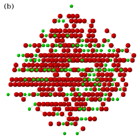
Figure 2: (a) Dynamic structure factor and (b) stratification (at the end of the simulation) of a BM configuration of linear size $L=10$ with density $\rho=0.535$.

In order to clarify what type of restructuring is occurring, we visualize an exemplar BM system at some late instance of the simulation in fig. 2. The picture clearly shows that the system has reorganized itself into a stratified structure along a direction close to the body diagonal of the cubical sample we considered, in agreement with the directions along which the structure factor grows. Both samples of linear size $L=10$ and $L=30$ reveal this alternation of several more densely populated planes with usually one that is less occupied. However, given the irregularity of the alternation, it does not seem that the observed stratification is the beginning of an overall crystallization of the system, nor does a closer investigation with the naked eye allow to identify any recurring structure along these planes.

Figure 3: Average number of neighbors of particles ($\square$) and average number of mobile particles ($+$) in function of the total running time for a system of linear size $L=10$ with density $\rho=0.535$.

Even though the system does not go through a complete crystallization, it is important to consider what consequences this restructuring has on the systems dynamics. Therefore, we compute the average number of neighbors of each particle $\rho_{\mbox{\tiny{nn}}}(t)$ and the overall density of mobile particles $\rho_{\mbox{\tiny{mobile}}}(t)$, i.e., particles which are allowed to move to one of the neighboring empty sites, as a function of time $t$. We present these quantities in fig. 3, for the smaller system with $L=10$. We see that on average the number of neighbors of a particle undergoes a considerable decrease during the same time interval where the dynamic structure factor grows. Also in that same time region, the density of mobile particles $\rho_{\mbox{\tiny{mobile}}}$ increases. After this, both quantities still fluctuate, but basically the system maintains its newly acquired mobility. Thus, the stratification results in a structure where, on average, particles have less neighbors. As a consequence, they are less constrained, hence more of them become mobile. It is important to note that the larger amount of mobile particles is not just a simple reflection of the resulting reduced $3D$ layered structures. Though they originate from the restructuring of the system, they are a characteristic of the whole system.

This allows us to explain what is really happening during the initially observed acceleration of older systems described in the previous section. We have just shown that because the system is restructuring it gains in mobility. Thus, in general, older systems will be characterized by a higher overall mobility for short elapsed times $t-t_{\mbox{\tiny{w}}}$ and initially they will decay faster than younger, less mobile systems. However, once this initial time interval has been overcome, i.e., the system has restructured in order to become mobile, older systems decorrelate slower than younger ones. Hence, there must be some explanation, other than this stratification, as to why we observe the slower decorrelation of older systems at larger times, as discussed in the previous section.

5 Intrinsically Heterogeneous Dynamics

A quantity which typically reveals the degree to which glasses are dynamically heterogeneous, is the $4$-point susceptibility, defined as the variance of the correlation function,

$$\chi_{4}(t,t_{\mbox{\tiny{w}}})\equiv V\times\left(\langle C(t,t_{\mbox{\tiny{w}}})^{2}\rangle-\langle C(t,t_{\mbox{\tiny{w}}})\rangle^{2}\right)\;.$$ (2)

A rigorous analysis of the theoretically expected behavior for $\chi_{4}(t)$ is given in [14]. In full generality, it is possible to distinguish several time regimes during which the dynamic susceptibility usually follows a power-law, $\chi_{4}(t)\sim t^{\mu}$. Here, the actual value of the parameter $\mu$ depends strongly on the dominating relaxation mechanism. We shall compare our results with these predictions and extend the discussion to the dependency on the waiting time, for which –to our knowledge– there are no such qualitative predictions available yet.

Figure 4: Four-point dynamic susceptibility $\chi(t,t_{\mbox{\tiny{w}}})$ in function of the logarithm of the elapsed time $t-t_{\mbox{\tiny{w}}}$ since the waiting time $t_{\mbox{\tiny{w}}}$, for systems of linear size $L=10$ with density $\rho=0.535$. At large elapsed times, the curves correspond to systems of increasing ages from bottom to top.

We present the two-time temporal behavior for systems of linear size $L=10$ and density $\rho=0.535$ in fig. 4. During a small initial (elapsed) time window, the dynamic susceptibility grows according to a power law with $\mu\simeq 0.6$. This is in reasonable agreement with the $\mu=0.5$ prediction by [14] for the elastic regime. For such an elastic regime we expect no dependency on the age of the system, as is confirmed by our results.

The subsequent time regime is marked again by a power-law, but now with $\mu\sim 0.2$. This matches the early $\beta$-regime and the subsequent plateau described by mode-coupling theory (MCT) for the correlation function. Although, we do not have any prediction for the MCT-parameters for the BM model, the local structural relaxation associated to the $\beta$-regime explains the observed behavior. Also, it is in this time window that the acceleration of older systems was observed, though it is no longer visible for the dynamic susceptibity. In fact, if it is just due to the way in which we prepare our BM system, it should not be strongly sample dependent and therefore not contribute to the variation of the correlation function.

Conversely, the next regime is distinguishable by the fact that the susceptibility does become dependent on both $t$ and $t_{\mbox{\tiny{w}}}$. In fact, this regime sets in at a time of the order of $t_{A}(t_{\mbox{\tiny{w}}},\rho)$. In MCT we can map this with the late $\beta$-regime which continues into the so-called $\alpha$-regime. In fact, one expects the system to become increasingly two-time dependent when the system relaxes in an increasingly collective manner. From the correlation function it was clear that older systems relax a lot slower than their younger counterparts. If the slow dynamics is cooperative in nature, we expect older systems to have an increasingly higher value for the dynamic susceptibility. Indeed, fig. 4 confirms that older systems are increasingly more dynamically heterogeneous during this regime.

The three time windows described up to now exist and are well defined for all systems that we have investigated. The remainder of the discussion, however, is observed only for smaller, less dense systems and hence those which completely loose their memory during our running time. Larger and denser systems do not decorrelate completely during our simulations, but neither does the dynamic susceptibility peak during our running time. Rather, for the latter $\chi_{4}(t)$ is only observed to grow.

For the system represented in fig. 4 the growth of $\chi_{4}(t,t_{\mbox{\tiny{w}}})$ continues up to some time $t^{*}-t_{\mbox{\tiny{w}}}$ for systems of any age. Though we cannot say with certainty that the time at which $\chi_{4}(t)$ peaks, i.e., for $t^{*}-t_{\mbox{\tiny{w}}}\sim 2^{19}$, is independent of the age of the system, it seems to be less influenced than the value of $\chi_{4}$ at the peak itself. Being the time at which we observe the system has completely decorrelated and given the log-scale this is not so surprising though. In line with expectation of the preceding time window, the peak of $\chi_{4}$ is larger for older systems indicating that the latter are more dynamically heterogeneous after shorter elapsed times.

After having peaked, the susceptibility decreases and reaches a constant value when the system has thermalized. Although [14] suggested the subsequent decay should be very fast, it is not clear to us why this should necessarily be the case. At least for BM we find the subsequent decay to follow again a power-law, characterized by a largely $t_{\mbox{\tiny{w}}}$-independent value for $\mu\sim 0.2$. This indicates the system is probably already closer to its steady state. In fact, the final value of the susceptibility, reached within our running time by the younger systems, is lower than the peak-value, but higher than one, the value predicted for lattice gases with trivial equilibrium [3]. The limit of the susceptibility for the BM model, which has non trivial equilibrium configurations, is not so easily calculated. However, from our simulations, we find that it reaches a constant value, which is density and waiting time dependent. The exact dependence on the density of this limiting value is not clear, though it seems to grow with density. In any case, it suggests that the BM system is inherently dynamically heterogeneous. This is also supported by the fact that the final value of the susceptibility of older systems is larger than that of younger ones.

6 Conclusions

In this paper, we have analyzed the dynamical behavior of the thermodynamically defined BM lattice glas model. We have found some interesting ageing behavior, and we have discussed its connections with the non trivial topology of the energy landscape of these models. We have analyzed the real space behavior of the model and found signs of a layered structure emerging with time. The reorganized structure is however not reflected in the mobility of the particles. The dynamics is observed to be increasingly heterogeneous for older systems. Moreover, when the system has lost its memory of the initial configuration, the $4$-point-susceptibility assumes a density-dependent constant value suggesting an important role of intrinsic heterogeneities in the model. A comparison with predictions of [14] is very successful for a large number of features. It only breakes down regarding the rate of decay after the susceptibility peaks: this is one of the points that obviously calls for further clarification.

- [1] \NameCugliandolo L. F. \Bookin Slow relaxations and nonequilibrium dynamics in condensed matter \Vol77 \PublSpringer, Berlin \Year2003 \Page769.
- [2] \NameEdiger M. D. \REVIEWAnnu. Rev. Phys. Chem.51200099.
- [3] \NameRitort F. Sollich P. \REVIEWAdvances in Physics522003219.
- [4] \NameKob W. Andersen H. \REVIEWPhys. Rev. E4819934364.
- [5] \NameFranz S., Mulet R. Parisi G. \REVIEWPhys. Rev. E652002021505.
- [6] \NameToninelli C., Biroli G. Fisher D. S. \REVIEWPhys. Rev. Lett.922004185504.
- [7] \NameMarinari E. Pitard E. \REVIEWEurophys. Lett.692005235.
- [8] \NameBiroli G. Mézard M. \REVIEWPhys. Rev. Lett.882002025501.
- [9] \NameMcCullagh G. D., Cellai D., Lawlor A. Dawson K. A. \REVIEWPhys. Rev. E712005030102.
- [10] \NameBiroli G. \REVIEWJ. Stat. Mech.200505014.
- [11] \NameKurchan J., Peliti L. Sellitto M. \REVIEWEurophys. Lett.391997365.
- [12] \NameSellitto M. \REVIEWJ. Phys.:Condens. Matter1420021455.
- [13] \NameCavagna A., Giardina I. Grigera T. S. \REVIEWEurophys. Lett.61200374.
- [14] \NameToninelli C., Wyart M., Berthier L., Biroli G. Bouchaud J. \REVIEWPhys. Rev. E712005041505.