Generalized cell/dual-cell transformation for percolation, and new exact thresholds

Abstract

Suggested by Scullard’s recent star-triangle relation for correlated bond systems, we propose a general “cell/dual-cell” transformation, which allows in principle an infinite variety of lattices with exact percolation thresholds to be generated. We directly verify Scullard’s new site percolation thresholds, and derive the bond thresholds for his “martini” lattice ($p_{c}=1/\sqrt{2}$) and the “A” lattice ($p_{c}=0.625457\ldots$, solution to $p^{5}-4p^{4}+3p^{3}+2p^{2}-1=0$). We also present a precise Monte-Carlo test of the site threshold for the “A” lattice.

I Introduction

Percolation refers to the process of the formation of long-range connectivity in random systems StaufferAharony . It has wide-ranging applications to problems in physics and engineering, including conductivity and magnetism in random systems, fluid flow in porous media, epidemics and clusters in complex networks, and gelation in polymer systems. To study this phenomenon, one typically models the network by a regular lattice made random by independently making sites or bonds occupied with a probability $p$. At a critical threshold $p_{c}$, for a given lattice and percolation type (site, bond), percolation takes place. Finding that threshold exactly or numerically to high precision is essential to studying the percolation problem on a particular lattice.

There are in fact relatively few lattices where $p_{c}$ is known exactly, all in two dimensions, where a powerful duality-crossing argument can be used. These lattices include bond percolation on the square lattice and site percolation on the triangular lattice (both with $p_{c}=1/2$), and a family of related lattices (bond-triangular, bond-honeycomb, site-kagomé, site-(3,12²)) whose non-trivial thresholds can be found though the star-triangle transformation introduced by Sykes and Essam SykesEssam . This transformation was successfully applied to one other lattice (the “bowtie” lattice, bond percolation) by Wierman Wierman .

Very recently Scullard has shown that the star-triangle relation can be generalized to situations where the bonds in the triangular unit have correlations among them Scullard . He argued that a specific correlated system could be represented by uncorrelated site percolation on certain lattices, leading to exact percolation thresholds for three new lattices: his so-called “martini” lattice, and two related lattices, which we call “A” and “B”. Scullard’s proposed thresholds are $p_{c}(\hbox{site})=0.764826...$ (the solution to $p^{4}-3p^{3}+1=0$), $1/\sqrt{2}$, and $(\sqrt{5}-1)/2$, respectively. These rather startling results expand in a significant way the number and types of lattices where exact thresholds can be found.

In this paper, we show that Scullard’s arguments can be viewed in a more general way, in terms of the net correlation between the three vertices of a basic triangular cell. This correlation can be created by an arbitrary network of independent or correlated bonds, including groups of correlated bonds that effectively represent sites in the system. In this way, we derive the bond thresholds for the lattices Scullard considered (he already realized that the self-dual “B” lattice has a threshold of 1/2), give an alternative derivation of his site thresholds, and provide a prescription to generate additional lattices where the threshold can be found exactly. Finally, we report on numerical simulations to test Scullard’s prediction of $p_{c}(\hbox{site})$ for the “A” lattice.

II General criterion for percolation

We consider a lattice that can be decomposed into a regular triangular array of identical triangular cells as shown in Fig. 1a, where the shaded triangles represent any network of bonds, perhaps with correlations, that connect the three endpoints. Randomly occupied sites can also be included within the cell by incorporating triangles of correlated bonds. That that array is triangular as in Fig. 1a is not absolutely necessary (it need only be self-dual), but we will consider only the triangular array in this paper. The basic triangular cell has vertices $A$, $B$, and $C$, and we define $P(A,B,C)=$ the probability that $A$, $B$ and $C$ are all connected, $P(A,B,\overline{C})$ = the probablity that only $A$ and $B$ are connected, $P(\overline{A},\overline{B},\overline{C})=$ the probability that none of the three are connected, etc.

We find that the general criterion for criticality is simply

$$P(A,B,C)=P(\overline{A},\overline{B},\overline{C})$$ (1)

for an arbitrary triangular cell. This formula is analogous to one that is obtained for the triangular and honeycomb lattices via the star-triangle transformation, but generalized to apply to triangular cells with any number of bonds (including correlations), arranged in a self-dual pattern such as that in Fig. 1a.

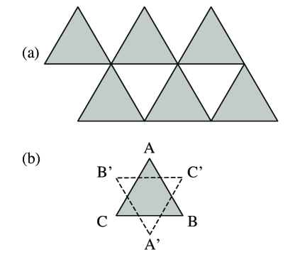
Figure 1: (a) Decomposition of lattice into cells (shaded), (b) the dual-cell transformation.

We derive this result using a generalized “cell/dual-cell” transformation. The development parallels that for the regular star-triangle transformation, but kept in a more general context. The dual system to Fig. 1a is also a regular triangular array of non-overlapping triangles (rotated by 180^∘). Call the vertices $A^{\prime}$, $B^{\prime}$, and $C^{\prime}$ on the dual triangle, as shown in Fig. 1b, and let $P^{\prime}(A^{\prime},B^{\prime},C^{\prime})$ etc. represent the probabilities of connecting vertices on the dual triangular cells.

For the two systems to be identical, rotate the dual system so that $A=A^{\prime}$, $B=B^{\prime}$ and $C=C^{\prime}$. Evidently, the two systems will have the same connectivity between vertices if we have simultaneously

$$P(A,B,C) = P^{\prime}(A,B,C)$$ (2)

$$P(A,B,\overline{C}) = P^{\prime}(A,B,\overline{C})\quad(\times 3)$$ (3)

$$P(\overline{A},\overline{B},\overline{C}) = P^{\prime}(\overline{A},\overline{B},\overline{C})$$ (4)

Note that for the two systems to have the same connectivity, the underlying bond occupancy of the dual cell will be different than that of the original cell (in fact, $1-p_{i}$ for a system of independent bonds), but we don’t need to specify that in detail here.

First we note that the two-point connectivity relations (3) are automatically satisfied as a result of duality. We see from Fig. 1b that if $A$ and $B$ connect on the original triangular cell, then $A^{\prime}$ and $B^{\prime}$ must also connect on the dual cell. Likewise, duality also implies that $P(A,B,C)=P^{\prime}(\overline{A},\overline{B},\overline{C})$, and $P(\overline{A},\overline{B},\overline{C})=P^{\prime}(A,B,C)$. Then, from Eqs. (2) and (4), the general condition (1) follows. This indeed represents the critical point because the two systems have identical connectivities, and one is the dual of the other.

Eq. (1) is equivalent to the relation $P(v,h)+P(v,l,\overline{h})+P(h,l,\overline{v})-P(\overline{v},\overline{l},\overline{h})=0$ given by Scullard for a system of three correlated bonds, where $v$, $h$, and $l$ are the vertical, horizontal, and diagonal edges of the basic triangle drawn as a right triangle. From the identity $P(v,h)=P(v,h,l)+P(v,h,\overline{l})$, and associating $P(A,B,C)=P(v,h,l)+P(v,h,\overline{l})+P(v,l,\overline{h})+P(h,l,\overline{v})$ and $P(\overline{A},\overline{B},\overline{B})=P(\overline{v},\overline{l},\overline{h})$, it follows that (1) is satisfied. Note that in the present work we consider systems with correlations more general than those produced by three correlated bonds.

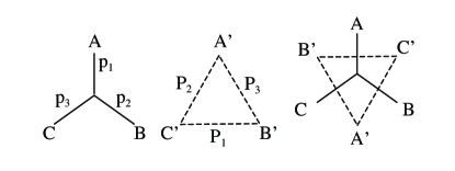
Figure 2: Star-triangle transformation. Left to right: star, triangle, duality orientation.

We illustrate explicitly our argument using the usual star-triangle transformation shown in Fig. 2. Here we will assume that the bond occupation probabilities are $p_{1}$, $p_{2}$ and $p_{3}$ on the star (the original cell), and $P_{1}$, $P_{2}$, and $P_{3}$ on the triangle (the dual cell). Then we have explicitly for Eqs. (2–4)

$$p_{1}p_{2}p_{3} = P_{1}P_{2}P_{3}+P_{1}P_{2}Q_{3}+P_{1}P_{3}Q_{2}+P_{2}P_{3}Q_{1}$$ (5)

$$p_{1}p_{2}q_{3} = Q_{1}Q_{2}P_{3}\quad(\times 3)$$ (6)

$$q_{1}q_{2}q_{3} + q_{1}p_{2}p_{3}+q_{2}p_{1}p_{3}+q_{3}p_{1}p_{2}=Q_{1}Q_{2}Q_{3}$$ (7)

where $q_{i}=1-p_{i}$ and $Q_{i}=1-P_{i}$. The two-point relation (6) is identically satisfied if $P_{i}=1-p_{i}$. Then, there follows from either (5) or (7) the condition $p_{1}p_{2}p_{3}-p_{1}p_{2}-p_{1}p_{3}-p_{2}p_{3}+1=0$, which for $p_{1}=p_{2}=p_{3}=p$ gives $p^{3}-3p^{2}+1=0$ or $p_{c}=1-2\sin\pi/18=0.652704\ldots$ for bond percolation on the honeycomb lattice SykesEssam .

Above we repeated the complete argument to find $p_{c}$, working out probabilities on the dual as well as the original system. But using (1), we could just as well equate $P(A,B,C)=p_{1}p_{2}p_{3}$ to $P(\overline{A},\overline{B},\overline{C})=q_{1}q_{2}q_{3}+q_{1}p_{2}p_{3}+q_{2}p_{1}p_{3}+q_{3}p_{1}p_{2}$ to find the same result without resorting explicitly to the dual lattice.

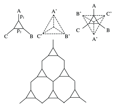
Figure 3: Cell, dual-cell, duality construction, and representation for Scullard’s “martini” lattice (bond percolation).

III The martini lattice (bond percolation)

Now we consider some new systems. First we consider the unit cell shown in Fig. 3, which is a triangle within a star. As shown in that figure, this cell forms precisely Scullard’s martini lattice, which is a honeycomb lattice with triangles inserted in every other site. Here we are considering bond percolation on that lattice. We will assume that the outer three bonds are each occupied with an equal probability $p_{1}$, and the inner three bonds are each occupied with probability $p_{2}$. Then a straightforward calculation shows that

$$P(A,B,C) = p_{1}^{3}(p_{2}^{3}+3p_{2}^{2}q_{2})$$ (8)

$$P(A,B,\overline{C}) = p_{1}^{2}q_{1}(p_{2}+q_{2}p_{2}^{2})+p_{1}^{3}(p_{2}q_{2}^{2})$$ (9)

$$P(\overline{A},\overline{B},\overline{C}) = q_{1}^{3}+3q_{1}^{2}p_{1}+3q_{1}p_{1}^{2}(q_{2}^{3}+2p_{2}q_{2}^{2})+p_{1}^{3}(q_{2}^{3})$$ (10)

Equating (8) and (10), we find

$$2p_{1}^{3}p_{2}^{3}-3p_{1}^{3}p_{2}^{2}-3p_{1}^{2}p_{2}^{3}+3p_{1}^{2}p_{2}^{2}+3p_{1}^{2}p_{2}-1=0$$ (11)

When $p_{1}=1$, this corresponds to a triangular lattice, and when $p_{2}=1$, a honeycomb lattice. When $p_{1}=p_{2}=p$, we have $(2p^{2}-1)(p^{4}-3p^{3}+2p^{2}+1)=0$ which yields $p_{c}=1/\sqrt{2}$, a new result. Interestingly, this is the same value as the site percolation threshold Scullard found for the “A” lattice discussed below (which is not the covering lattice of the martini lattice).

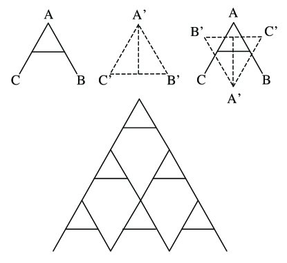
Figure 4: Cells and construction for bond percolation on the “A” lattice.

It is instructive to also work this out explicitly using the dual cell, which is a star within a triangle as shown in Fig. 3. Here $P_{1}$ is the occupancy of the outer bonds and $P_{2}$ is that of the inner bonds. We find

$$P^{\prime}(A,B,C) = P_{1}^{3}+3P_{1}^{2}Q_{1}+3P_{1}Q_{1}^{2}(P_{2}^{3}+2P_{2}^{2}Q_{2})+Q_{1}^{3}(P_{2}^{3})$$ (12)

$$P^{\prime}(A,B,\overline{C}) = P_{1}Q_{1}^{2}(Q_{2}+P_{2}Q_{2}^{2})+Q_{1}^{3}(P_{2}^{2}Q_{2})$$ (13)

$$P^{\prime}(\overline{A},\overline{B},\overline{C}) = Q_{1}^{3}(Q_{2}^{3}+3Q_{2}^{2}P_{2})$$ (14)

Then $P(A,B,\overline{C})=P^{\prime}(A,B,\overline{C})$ if $Q_{i}=p_{i}$, and equating either $P(A,B,C)=P^{\prime}(A,B,C)$ or $P(\overline{A},\overline{B},\overline{C})=P^{\prime}(\overline{A},\overline{B},\overline{C})$ leads to the threshold given by (11).

Now, we can see that the transformation shown in Fig. 3 of the star-within-a-triangle to a triangle-within-a-star is analogous to the star-triangle transformation, but intrinsically different in that that transformation of Fig. 3 cannot be accomplished by applying the usual star-triangle transformation. This is an example of a more general cell/dual-cell transformation that can be applied to percolation problems, where the cell can be any graph connecting three vertices, and perhaps containing correlated bonds.

IV The “A” and “B” lattices (bond percolation)

In the same way, we can find $p_{c}(\hbox{bond})$ for the other two lattices considered by Scullard. In Fig. 4 we show what we call the “A” lattice, since the basic cell has the shape of an A. It is equivalent to the cell of the martini lattice with the upper bond removed or made occupied with probability 1. For simplicity, we assume all bonds are occupied with equal probablity $p$. We find

$$P(A,B,C) = p^{2}(p^{3}+3p^{2}q)$$ (15)

$$P(\overline{A},\overline{B},\overline{C}) = p^{2}(q^{3})+2pq(q^{3}+2pq^{2})+q^{2}$$ (16)

Equating the two, we find $p^{5}-4p^{4}+3p^{3}+2p^{2}-1=0$ , whose solution gives $p_{c}(\hbox{bond})=0.625457\ldots$. This threshold is also new.

Fig. 4 also shows the dual cell — a triangle with a vertical line in it — and once again, this defines a new cell/dual-cell transformation, and one can verify directly that $P(A,B,\overline{C})=P^{\prime}(A,B,\overline{C})$ with $P=1-p$, and rederive the above result for $p_{c}$.

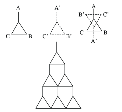
Figure 5: Construction for bond percolation on the “B” lattice.

Scullard’s third lattice is generated by the cell shown in Fig. 5, which corresponds to the martini generator with two bonds removed. We call this the “B” lattice, because the appearance of B’s when rotated by 90^∘, and also because it follows the “A” lattice. Because this lattice is self-dual, its $p_{c}(\hbox{bond})$ equals 1/2 as noted by Scullard. This result is also borne out by (1), since here

$$P(A,B,C) = p(p^{3}+3p^{2}q)$$ (17)

$$P(\overline{A},\overline{B},\overline{C}) = q(q^{3}+3q^{2}p)$$ (18)

Equating the two, one indeed finds $(2p-1)(p^{2}-p-1)=0$, implying $p_{c}=1/2$.

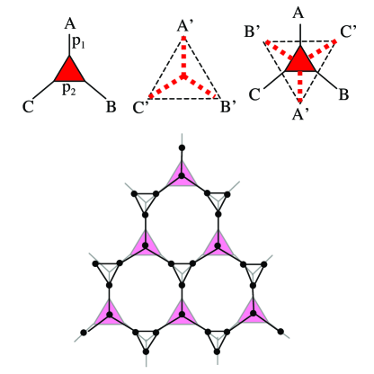
Figure 6: Construction for site percolation on the martini lattice, which is the covering lattice shown in the lower part of the figure (color online).

V Site percolation

Now, we turn to some site percolation models. In general, some (but not all) site percolation lattices can be created by constructing the covering lattice of a bond problem. Here we extend this procedure by also allowing for some of the bonds to be correlated. Thus in Fig. 6 we show a unit cell similar to that of Fig. 3 except that now the three central bonds are all simultaneously occupied with probability $p$, and all vacant otherwise. This is indicated by coloring the triangle enclosed by those bonds. Note that this triangle can also be thought of as simply an independently occupied site, showing that this is essentially a site-bond problem, in which context this problem was first solved by Kondor Kondor . Related correlated site-bond problems were also considered by Hu Hu and Wu Wu . In a somewhat different context, Kunz and Wu also used the idea of creating site percolation by a group of correlated bonds in bond percolation system KunzWu .

Let $p_{1}$ be the occupancy of the three outer bonds, and $p_{2}$ be the simultaneous occupancy of all three central bonds. The covering lattice (which corresponds to the equivalent pure site system) is exactly the martini lattice, as shown in Fig. 6. We find

$$P(A,B,C) = p_{1}^{3}p_{2}$$ (19)

$$P(\overline{A},\overline{B},\overline{C}) = q_{2}+p_{2}(q_{1}^{3}+3p_{1}q_{1}^{2})$$ (20)

and setting these equal yields $(p_{1}^{3}-3p_{1}^{2})p_{2}+1=0$ as given by Kondor Kondor . Setting $p_{1}=p_{2}=p$ yields $p^{4}-3p^{3}+1=0$ or $p_{c}=0.764826\ldots$ for site percolation on the martini lattice, as found by Scullard. Here, the dual lattice is a triangle with a correlated star in the center, and one can verify directly that the two-point functions on the lattice and dual lattice are equal when $P_{i}=1-p_{i}$.

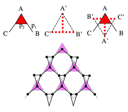
Figure 7: Construction for site percolation on the “A” lattice (color online).

For site percolation on the “A” lattice the cell/dual cell combination is shown in Fig. 7. Here we have

$$P(A,B,C) = p_{1}^{2}p_{2}$$ (21)

$$P(\overline{A},\overline{B},\overline{C}) = q_{2}+p_{2}q_{1}^{2}$$ (22)

which yields $2p_{1}p_{2}-1=0$. When $p_{1}=p_{2}=p$ this yields $p_{c}=1/\sqrt{2}$ as found by Scullard. For site percolation on the “B” lattice, as shown in Fig. 8, we have $P(A,B,C)=p_{1}p_{2}$ and $P(\overline{A},\overline{B},\overline{C})=q_{2}$ yielding $(p_{1}+1)p_{2}-1=0$. For $p_{1}=p_{2}=p$, this yields $p_{c}=(\sqrt{5}-1)/2=0.618034\ldots.$ as found by Scullard.

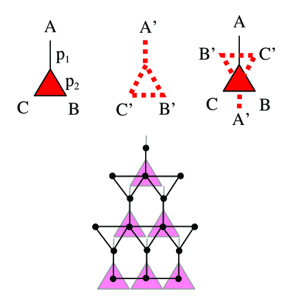
Figure 8: Construction for site percolation on the “B” lattice (color online).

Likewise, one can create other cells that generate additional lattices where $p_{c}$ can be found exactly. By making the cell simply a shaded triangle (all three bonds occupied together), we create the site-triangular problem. A cell of just two bonds creates the bond-square problem. A cell with three correlated triangles touching creates the site-kagomé problem. In this way, all known thresholds can be easily calculated, and an infinite number of new ones can be created, with additional lattices tending to be more and more intricate. Unfortunately, the method does not appear to work for some of the more notorious unsolved systems: site percolation on the square and honeycomb lattices, and bond percolation on the kagomé lattice.

An example of an intrinsically correlated system is one in which the cell is a simple triangle of bonds but where we require that in each cell at least one bond is occupied, so that $P(\overline{A},\overline{B},\overline{C})=0$. Eq. (1) implies that at criticality $P(A,B,C)=0$ also, so that the only non-zero correlation is $P(A,B,\overline{C})$ and permutations, meaning that the critical point corresponds to all cells having exactly one occupied bond (in either a random or biased location), yielding $p_{c}=1/3$. If only two of the three bonds can be occupied, then the threshold corresponds to exactly one of those two being occupied ($p_{c}=1/2$), and we find a Scheidegger’s river network model Scheidegger , many of whose properties have been studied and solved (e.g., TakayasuNishikawaTasaki ; Huber ). These are examples of fixed number or canonical percolation models.

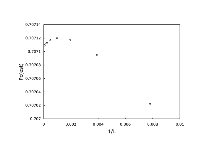
Figure 9: Hull-gradient simulation results for site percolation on the “A” lattice, confirming Scullard’s prediction $p_{c}=1/\sqrt{2}\approx 0.707107$. Error bars are smaller than the symbol size.

VI Numerical test for site percolation on the “A” lattice”

Finally, we report the results of a numerical test of $p_{c}(\hbox{site})$ for the “A” lattice, whose threshold was predicted to be $1/\sqrt{2}=0.70710678\ldots$ Scullard . We used the hull-gradient method ZiffSapoval ; SudingZiff , with the lattice represented on a square lattice as $2\times 2$ squares with a diagonal in the left-lower corner. We considered systems of width $L=128,256,\ldots 16384$ with the gradient $=1/L$. The estimates of $p_{c}$ (equal to the ratio of occupied to total sites in the hull) are plotted in Fig. 9 vs. $1/L$, with $10^{12}-10^{13}$ sites generated for each $L$. For $L=16384$, we find $p_{c}(\hbox{est})=0.7071090$, and the data extrapolate to the expected value as $L\to\infty$ with a statistical error of about $\pm 0.000001$. Note that there are rather unusual finite-size effects for this system (perhaps related to the orientation/representation of the lattice) as the estimates first increase and then decrease as $L$ increases.

We did not check any of the other predictions numerically: because the cell/dual-cell argument is so compelling, there seems to be little doubt that these results are correct.

VII Conclusions and Discussion

We have shown that the well-known star-triangle transformation usually applied to honeycomb/triangular lattices is a special case of a generalized transformation where triangular cells in a system are individually replaced by their duals. When the triangles themselves form a self-dual system as in Fig. 1a, then the generalized criterion for percolation (1) follows. Interestingly, to apply this criterion one does not need to explicitly apply the star-triangle or duality transformation, as the criterion involves connectivity probabilities on just the original system.

Note that Fig. 1a is but one arrangement of the triangular cells that is self dual. Other arrangements can also be devised, and these will be pursued in future work.

The basic triangular cells can possess correlations in their connectivities, and we have shown that correlations can be the result of having an uncorrelated bond system that is more complicated than a simple triangle or star. Site percolation can also be included by adding triangles of correlated bonds. In this way, we have provided a direct proof of Scullard’s new results for the site percolation threshold for the martini lattice, and its two contractions, the “A” and “B” lattices. We derived the bond thresholds of these lattices also, which represents two additional new thresholds. Note that these three lattices are the only known cases, besides the triangular lattice, where both site and bond percolation thresholds can be found exactly. Other soluble lattices can easily be generated by putting additional bonds on the basic cells, although the lattices thus formed take on more and more the look of “decorated” rather than regular lattices.

It turns out that the criterion that we derived, Eq. (1), is closely related to work done many years ago on the Potts model in correlated systems fywuPrivateComm . In fact, (1) is a special case of a criterion for being at the critical point of the correlated Potts model given by Wu and co-workers WuLin ; WuZia ; MaillardRolletWu ; KingWu . However, evidently the percolation limit of that work was never explored.

Finally, after this paper was submitted for publication, we came across a recent preprint of work by Chayes and Lei Chayes in which the generalized criterion (1) was also derived. The focus of their work is quite different, and these authors do not use that criterion to find the thresholds of new lattices as we have done here.

VIII Acknowledgments

The author thanks Chris Scullard for sending an advance copy of his paper and for a stimulating exchange of email correspondence, Greg Huber for discussions on river networks, and F. Y. Wu for comments and for assistance on the relation to previous work on the correlated Potts model. The author acknowledges financial support from NSF grant DMS-0244419.

References

- (1) D. Stauffer and A. Aharony, Introduction to Percolation Theory (Taylor and Francis, 1994).
- (2) M. F. Sykes and J. W. Essam, J. Math. Phys. 5, 1117 (1964).
- (3) J. C. Wierman, J. Phys. A 17, 1525 (1984).
- (4) C. Scullard, “Exact site percolation thresholds using a site-to-bond transformation and the star-triangle transformation,” Phys. Rev. E (to appear) (2006)
- (5) I. Kondor, J. Phys. C 13, L531 (1980).
- (6) C. K. Hu, Phys. Rev. B 29, 5103 (1984).
- (7) F. Y. Wu, J. Phys. A 14, L39 (1981).
- (8) A. E. Scheidegger, Bull. Int. Assoc. Sci. Hydrology 12, 15 (1967).
- (9) H. Takayasu, I. Nishikawa, and H. Tasaki, Phys. Rev. A 37, 3110 (1988).
- (10) G. Huber, Physica A 170, 463 (1991).
- (11) F. Y. Wu and K. Y. Lin, J. Phys. A 13, 629 (1980).
- (12) F. Y. Wu and R. K. P. Zia, J. Phys. A 14, 721 (1981).
- (13) C. King and F. Y. Wu, Int. J. Mod. Phys. B 11, 51 (1997).
- (14) J. M. Maillard, G. Rollet, and F. Y. Wu, J. Phys. A 26, L495 (1993).
- (15) H. Kunz and F. Y. Wu, J. Phys. C 11, L1, L357 (1977).
- (16) R. M. Ziff and B. Sapoval, J. Phys. A 19 L1169 (1986).
- (17) P. N. Suding and R. M. Ziff, Phys. Rev. E 60, 275 (1999).
- (18) F. Y. Wu, private communication
- (19) L. Chayes and H. K. Lei, “Random cluster models on the triangular lattice,” preprint arxiv:cond-mat/0508253, 10 August 2005.