Moment Equations for a Spatially Extended System of Two Competing Species

Abstract

The dynamics of a spatially extended system of two competing species in the presence of two noise sources is studied. A correlated dichotomous noise acts on the interaction parameter and a multiplicative white noise affects directly the dynamics of the two species. To describe the spatial distribution of the species we use a model based on Lotka-Volterra (LV) equations. By writing them in a mean field form, the corresponding moment equations for the species concentrations are obtained in Gaussian approximation. In this formalism the system dynamics is analyzed for different values of the multiplicative noise intensity. Finally by comparing these results with those obtained by direct simulations of the time discrete version of LV equations, that is coupled map lattice (CML) model, we conclude that the anticorrelated oscillations of the species densities are strictly related to non-overlapping spatial patterns.

I Introduction

The dynamics of real ecosystems is strongly affected by the presence of noise sources, such as the random variability of temperature, resources and in general environment, with which the system has a multiplicative interaction Zimmer ; Ciuchi . In this paper we analyze the time evolution of a spatially extended system formed by two competing species in the presence of two noise sources. We get the dynamics in the formalism of the moments. We study the role of the two noise sources on the ecosystem dynamics, described by generalized Lotka-Volterra equations in the presence of external fluctuations, modelled as multiplicative noise. Specifically we focus on the time behavior of the $1^{st}$ and $2^{nd}$ order moments of the species concentrations. We find that the $1^{st}$ order moments are independent on the multiplicative noise intensity. On the other hand the behavior of the $2^{nd}$ order moments is strongly affected by the presence of a source of external noise. We find anticorrelated time behavior of the species densities. Comparing our results with those obtained by calculating the same quantities within a coupled map lattice (CML) model Kaneko , we conclude that the anticorrelated oscillations of the species concentrations are strictly related to non-overlapping spatial patterns Spagnolo . Our theoretical results could match data from a real ecosystem, whose dynamics is affected by the random variability of the environment, and could provide useful tools to predict behavior of biological species Zimmer ; Ciuchi ; Spagnolo ; Garcia .

II The model

Our system is described by a time evolution model of Lotka-Volterra equations, within the Ito scheme, with diffusive terms in a spatial lattice with $N$ sites

$$\dot{x}_{i,j} = \mu x_{i,j}(1-x_{i,j}-\beta y_{i,j})+x_{i,j}\sqrt{\sigma_{x}}\xi^{x}_{i,j}+D\sum_{\gamma}(x_{\gamma}-x_{i,j})$$ (1)

$$\dot{y}_{i,j} = \mu y_{i,j}(1-y_{i,j}-\beta x_{i,j})+y_{i,j}\sqrt{\sigma_{y}}\xi^{y}_{i,j}+D\sum_{\gamma}(y_{\gamma}-y_{i,j}),$$ (2)

where $x_{i,j}$ and $y_{i,j}$ denote respectively the densities of species $x$ and species $y$ in the lattice site $(i,j)$, $\mu$ is the growth rate, $D$ is the diffusion constant, and $\sum_{\gamma}$ indicates the sum over all the sites. Here $\xi^{x}_{i,j}(t)$ and $\xi^{y}_{i,j}(t)$ are statistically independent Gaussian white noises with zero mean and unit variance, $\sigma_{x}$ and $\sigma_{y}$ are the intensities of the multiplicative noise which models the interaction between the species and the environment, and $\beta$ is the interaction parameter.

II.1 The interaction parameter

Depending on the value of the interaction parameter, coexistence or exclusion regimes take place. Namely for $\beta<1$ both species survives, while for $\beta>1$ one of the two species extinguishes after a certain time. These two regimes correspond to stable states of the Lotka-Volterra’s deterministic model Spagnolo ; Vilar-Spagnolo ; Valenti ; Valenti1 . Moreover periodical and random driving forces connected with environmental and climatic variables, such as the temperature, modify the dynamics of the ecosystem, affecting both directly the species densities and the interaction parameter. This causes the system dynamics to change between coexistence ($\beta<1$) and exclusion ($\beta>1$) regimes. To describe this dynamical behavior we consider as interaction parameter $\beta(t)$ a dichotomous stochastic process, whose jump rate is a periodic function $\gamma(t)$

$$\gamma(t)=\left\{\begin{array}[c]{ll}0,&\quad\Delta t\leq\tau_{d}\\ \gamma_{0}\left(1+A\thinspace|\cos\omega t|\right),&\quad\Delta t>\tau_{d}\;.\end{array}\right.$$ (5)

Here $\Delta t$ is the time interval between two consecutive switches, and $\tau_{d}$ is the delay between two jumps, that is the time interval after a switch, before another jump can occur. In eq. (5), $A$ and $\omega=(2\pi)/T$ are respectively the amplitude and the angular frequency of the periodic term, and $\gamma_{0}$ is the jump rate in the absence of periodic term. This causes $\beta(t)$ to jump between two values, $\beta_{down}<1$ and $\beta_{up}>1$, which correspond to the dynamical regimes of the deterministic Lotka-Volterra’s model (coexistence and exclusion regions). Because the dynamics of the species strongly depends on the value of the interaction parameter, we report in Fig. 1 the time series of $\beta(t)$ for different values of delay $\tau_{d}$, namely $\tau_{d}=10,43.5,60$, with $\beta_{down}=0.94$ and $\beta_{up}=1.04$.

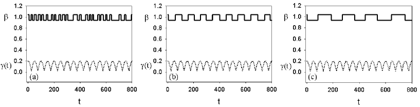
Figure 1: Time evolution of the interaction parameter $\beta(t)$ with initial value $\beta(0)=1.04$ and different values of delay: (a) $\tau_{d}=10$ (a), $43.5$ (b), and $80$ (c). The values of the other parameters are: $A=9.0$, $\omega/(2\pi)=10^{-2}$, $\gamma_{0}=2\cdot 10^{-2}$.

We note that the correlation time $\tau_{d}$ of the dichotomous noise affects the switch time between the two levels of $\beta(t)$. For a delay time a bit less than $T/2$, we observe a synchronization between the jumps and the periodicity of the rate $\gamma(t)$. This synchronization phenomenon is due to the choice of the $\tau_{d}$ value, which stabilizes the jumps in such a way they happen for high values of the jump rate, that is for values around the maximum of the function $\gamma(t)$. This causes a quasi-periodical time behavior of the species concentrations $x$ and $y$, which can be considered as a signature of the stochastic resonance phenomenon Benzi in population dynamics Vilar-Spagnolo ; Valenti ; Valenti1 . Therefore we fix the delay at the value $\tau_{D}=43.5$, corresponding to a competition regime with $\beta$ switching quasi-periodically from coexistence to exclusion regions (see Fig. 1b).

III Mean field model

In this section we derive the moment equations for our system. Assuming $N\rightarrow\infty$, we write Eqs. (1) and (2) in a mean field form

$$\dot{x} = f_{x}(x,y)+\sqrt{\sigma_{x}}g_{x}(x)\xi^{x}+D(<x>-x),$$ (6)

$$\dot{y} = f_{y}(x,y)+\sqrt{\sigma_{y}}g_{y}(y)\xi^{y}+D(<y>-y),$$ (7)

where $<x>$ and $<y>$ are average values on the spatial lattice considered (strictly speaking they are the ensemble average in the thermodynamics limit) and we set $f_{x}(x,y)=\mu x(1-x-\beta y)$, $g_{x}(x)=x$, $f_{y}(x,y)=\mu y(1-y-\beta x)$, $g_{y}(y)=y$. By site averaging Eqs. (6) and (7), we obtain

$$<\dot{x}>~{}=~{}<f_{x}(x,y)>,$$ (8)

$$<\dot{y}>~{}=~{}<f_{y}(x,y)>.$$ (9)

By expanding the functions $f_{x}(x,y)$, $g_{x}(x)$, $f_{y}(x,y)$, $g_{y}(y)$ around the $1^{st}$ order moments $<x>$ and $<y>$, we get an infinite set of simultaneous ordinary differential equations for all the moments Kawai . To truncate this set we apply a Gaussian approximation, for which the cumulants above the $2^{nd}$ order vanish. Therefore we obtain

$$<\dot{x}> = \mu<x>(1-<x>-\beta<y>)-\mu(\beta\mu_{11}+\mu_{20})$$ (10)

$$<\dot{y}> = \mu<y>(1-<y>-\beta<x>)-\mu(\beta\mu_{11}+\mu_{02})$$ (11)

$$\dot{\mu}_{20} = 2\mu\mu_{20}-2D\mu_{20}-2\mu\beta<y>\mu_{20}-2\mu<x>(\beta\mu_{11}+2\mu_{20})$$ (12)

$$+ 2\sigma_{x}(<x>^{2}+\mu_{20})$$

$$\dot{\mu}_{02} = 2\mu\mu_{02}-2D\mu_{02}-2\mu\beta<x>\mu_{02}-2\mu<y>(\beta\mu_{11}+2\mu_{02})$$ (13)

$$+ 2\sigma_{y}(<y>^{2}+\mu_{02})$$

$$\dot{\mu}_{11} = 2\mu\mu_{11}-2D\mu_{11}-<x>[2\mu\mu_{11}+\mu\beta(\mu_{11}+\mu_{02})]$$ (14)

$$- <y>[2\mu\mu_{11}+\mu\beta(\mu_{11}+\mu_{20})]~{},$$

where $\mu_{20}$, $\mu_{02}$, $\mu_{11}$ are the $2^{nd}$ order central moments defined on the lattice

$$\mu_{20} = <x^{2}>-<x>^{2}$$ (15)

$$\mu_{02} = <y^{2}>-<y>^{2}$$ (16)

$$\mu_{11} = <xy>-<x><y>~{}.$$ (17)

In order to get the dynamics of the two species we analyze the time evolution of the $1^{st}$ and $2^{nd}$ order moments according to Eqs. (10)-(14). We fix the delay time at the value $\tau_{d}=43.5$, corresponding to a quasi-periodic switching between the coexistence and exclusion regimes, and we obtain the time series of the moments for two values of the multiplicative noise intensity $\sigma=\sigma_{x}=\sigma_{y}$, namely $\sigma=10^{-12}$, $10^{-6}$, and in the absence of it. The values of the parameters are $\mu=2$, $D=0.05$. The initial values of the moments are $<x(0)>$ = $<y(0)>$ = $0.1$, $\mu_{20}(0)=\mu_{02}(0)=\mu_{11}(0)=0$. These initial conditions correspond to uniformly distributed species on the lattice considered.

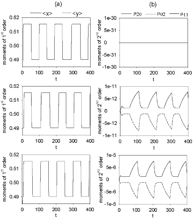
Figure 2: Time evolution of the $1^{st}$ and $2^{nd}$ order moments. The time series of (a) $<x(t)>$ and $<y(t)>$, and (b) $\mu_{2,0}$ and $\mu_{0,2}$ respectively, are completely overlapped. The values of the multiplicative noise intensity are: $\sigma=0,10^{-12},10^{-6}$, from top to bottom. Here $\tau_{d}=43.5$, $\mu=2$, and $D=0.05$. The initial values of the moments are $<x(0)>$ = $<y(0)>$ = $0.1$, $\mu_{20}(0)=\mu_{02}(0)=\mu_{11}(0)=0$. The values of the other parameters are the same of Fig. 1.

In Fig. 2 we note that the $1^{st}$ order moments of both species oscillate together quasi regularly around $0.5$, independently on the multiplicative noise intensity (see Fig. 2a). The noise intensity affects strongly the dynamics of the $2^{nd}$ order moments. In the absence of noise $\mu_{20}$, $\mu_{02}$, $\mu_{11}$ are zero. For very low levels of multiplicative noise ($\sigma=10^{-12}$) quasi-periodical oscillations appear with the same frequency of the interaction parameter $\beta(t)$, because the noise breaks the symmetry of the dynamical behavior of the $2^{nd}$ order moments (see Fig. 2b) Valenti . The time behavior of the variances of x and y species coincides all the time with alternating periods, characterized by small (close to zero) and large values. However the negative values of the correlation $\mu_{11}$ indicate that the two species distributions are anti-correlated. This means that the spatial distribution in the lattice will be characterized by zones with a maximum of concentration of species $x$ and a minimum of concentration of species $y$ and viceversa. The two species will be distributed therefore in non-overlapping spatial patterns. This physical picture is in agreement with previous results obtained with a different model  Valenti1 . For higher levels of multiplicative noise ($\sigma=10^{-6}$) the amplitude of the oscillations increases both in $\mu_{20}$, $\mu_{02}$ and $\mu_{11}$. This gives information on the probability density of both species, whose width and mean value undergo the same oscillating behavior. The anti-correlated behavior is enhanced by increasing the noise intensity value (see Figs. 2b). We note that the amplitude of the oscillations in Fig. 2b increases with the noise intensity $\sigma$ and it is of the same order of magnitude. The periodicity of these noise-induced oscillations shown in Fig. 2 is the same of the interaction parameter $\beta(t)$ (see Fig. 1). Even if it is due to a very different mechanism, this behavior is similar to the stochastic resonance effect produced in population dynamics, when the interaction parameter is subjected to an oscillating bistable potential in the presence of additive noise Valenti ; Valenti1 . We note that in the absence of external noise ($\sigma=0$) both populations coexist and the species densities oscillate in phase around their stationary value Valenti . This occurs identically in each site of the spatial lattice. The behavior of the mean value therefore will reproduce this situation. For $\sigma\neq 0$, anticorrelated oscillations appear due to the multiplicative noise, superimposed to the average behavior obtained for $\sigma=0$ and distributed randomly in the spatial structure. By site averaging these noise-induced oscillations (see Ref. Valenti ) we recover the average behavior obtained in the absence of noise. This explains why the first moment behavior is independent on the external noise intensity.

IV Coupled Map Lattice Model

In order to check our results we consider a different approach to analyze the dynamics of our spatial extended system. We consider the time evolution of CML model, which is the discrete version of the Lotka-Volterra equations with diffusive terms. For this model we found anticorrelated spatial patterns of the two competing species Valenti1 , that are related to the dynamical behavior of the moments of the species densities. Here we calculate the moments in the CML model. Within this formalism, the dynamics of the spatial distribution of the two species is given by the following equations

$$x_{i,j}^{(n+1)} = \mu x_{i,j}^{(n)}(1-x_{i,j}^{(n)}-\beta^{(n)}y_{i,j}^{(n)})+\sqrt{\sigma_{x}}x_{i,j}^{(n)}\xi_{i,j}^{x{(n)}}+D\sum_{\gamma}(x_{\gamma}^{(n)}-x_{i,j}^{(n)}),$$ (18)

$$y_{i,j}^{(n+1)} = \mu y_{i,j}^{(n)}(1-y_{i,j}^{(n)}-\beta^{(n)}x_{i,j}^{(n)})+\sqrt{\sigma_{y}}y_{i,j}^{(n)}\xi_{i,j}^{y{(n)}}+D\sum_{\gamma}(y_{\gamma}^{(n)}-y_{i,j}^{(n)}),$$ (19)

where $x^{(n)}_{i,j}$ and $y^{(n)}_{i,j}$ denote respectively the densities of prey x and prey y in the site $(i,j)$ at the time step $n$, $\mu$ is the growth rate and $D$ is the diffusion constant. $\xi_{i,j}^{x(n)}$ and $\xi_{i,j}^{y(n)}$ are independent Gaussian white noise sources with zero mean and unit variance. The interaction parameter $\beta^{(n)}$ corresponds to the value of $\beta(t)$ taken at the time step $n$, according to Eq. (5). Here $\sum_{\gamma}$ indicates the sum over the four nearest neighbors. To evaluate the $1^{st}$ and $2^{nd}$ order moments we define on the lattice, at the time step $n$, the mean values $<x>_{{}_{CML}}^{(n)}$, $<y>_{{}_{CML}}^{(n)}$,

$$<z>_{{}_{CML}}^{(n)}~{}=~{}\frac{\sum_{i,j}z^{(n)}_{i,j}}{N}~{},\qquad z=x,y$$ (20)

the variances $var^{(n)}_{x}$, $var^{(n)}_{y}$

$$var^{(n)}_{z}=\sqrt{s^{(n)}_{z}}=\sqrt{\frac{\sum_{i,j}(z^{(n)}_{i,j}-<z>^{(n)})^{2}}{N}}~{},\qquad z=x,y$$ (21)

and the correlation coefficient $corr^{(n)}$ of the two species

$$corr^{(n)}=\frac{cov^{(n)}_{xy}}{s^{(n)}_{x}s^{(n)}_{y}},$$ (22)

with

$$cov^{(n)}_{xy}=\frac{\sum_{i,j}(x^{(n)}_{i,j}-<x>^{(n)})(y^{(n)}_{i,j}-<y>^{(n)})}{N}.$$ (23)

The number of lattice sites is $N=100\times 100$. The time behavior of these quantities, for two levels of the multiplicative noise and in the absence of it, is reported in Fig. 3.

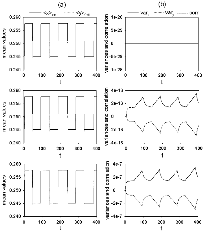
Figure 3: (a) Mean values: $<x>_{{}_{CML}}$, $<y>_{{}_{CML}}$, and (b) variances: $var_{x}$, $var_{y}$ and $corr$ of the two species, as a function of time. The values of the multiplicative noise intensity are: $\sigma=0,10^{-12},10^{-6}$, from top to bottom. The initial values of the species concentrations are $x_{i,j}^{(0)}=y_{i,j}^{(0)}=0.1$ for all sites $(i,j)$. The values of the other parameters are the same of Fig. 2.

The $1^{st}$ and $2^{nd}$ order moments of Eqs. (20)- (23) correspond respectively to the same quantities shown in Fig. 2. We note that the two set of time series are in a good qualitative agreement. The discrepancies in the oscillation intensities are due to the different values of the stationary values of the species densities in the considered models. Specifically: $x_{st}=y_{st}=\alpha/(1+\beta)\simeq 0.5$ for the mean field model, and $x_{st}^{n}=y_{st}^{n}=(1-1/\mu)/(1+\beta^{n})\simeq 0.25$ for the CML model. Moreover the behavior of the $2^{nd}$ order moments in Fig. 3b shows little irregularities with respect to that obtained in the mean field model, because the species interaction in the CML model is restricted to the nearest neighbors.

V Conclusions

We report a study on the dynamics of a spatially extended ecosystem of two competing species, described by generalized Lotka-Volterra equations. Two noise sources are present: a multiplicative white noise, which affects directly the two species densities, and a correlated dichotomous noise, which produces a random interaction parameter whose values jump between two levels. The role of the dichotomous correlated noise is to control the dynamical regime of the ecosystem (see Fig. 1), while the multiplicative noise is responsible for the anticorrelated behavior of the species concentrations (see time behavior of $\mu_{11}$ in Figs. 2b and 3b). The anti-correlated oscillations are enhanced by increasing the multiplicative noise intensity. The mean field approach with the Gaussian approximation enables us to obtain the time behavior of the $1^{st}$ and $2^{nd}$ order moments, which characterize the spatio-temporal behavior of the ecosystem. We compare the results obtained within a mean field approach with those obtained with a CML model. The agreement is quite good and allows us to conclude that the spatial patterns of the two species, within the mean field approach, should be non-overlapping as those obtained with the CML model Valenti1 . Our theoretical results could explain the time evolution of populations in real ecosystems whose dynamics is strictly dependent on noise sources, which are always present in the natural environment Garcia ; Caruso ; Sprovieri .

VI Acknowledgments

This work was supported by ESF (European Science Foundation) STOCHDYN network and partially by MIUR.

References

- (1) Special section on Complex Systems, Science 284, 79 (1999); C. Zimmer, Science, 284 (1999) 83; O. N. Bjornstad and B. T. Grenfell, Science 293, 638 (2001).
- (2) S. Ciuchi, F. de Pasquale and B. Spagnolo, Phys. Rev. E 53, 706 (1996); M. Scheffer et al., Nature 413, 591 (2001); A. F. Rozenfeld et al., Phys. Lett. A 280, 45 (2001).
- (3) Special issue CML models, edited by K. Kaneko [Chaos 2, 279– (1992)].
- (4) B. Spagnolo, D. Valenti, A. Fiasconaro, Math. Biosciences and Engineering 1, 185-211 (2004).
- (5) J. García Lafuente, A. García, S. Mazzola, L. Quintanilla, J. Delgado, A. Cuttitta and B. Patti, Fishery Oceanography 11, 31 (2002).
- (6) J. M. G. Vilar and R. V. Solé, Phys. Rev. Lett. 80, 4099 (1998); B. Spagnolo and A. La Barbera, Physica A 315, 114-124 (2002); A. La Barbera and B. Spagnolo, Physica A 315, 201 (2002); B. Spagnolo, A. Fiasconaro, D. Valenti, Fluc. Noise Lett. 3, L177 (2003).
- (7) D. Valenti, A. Fiasconaro, B. Spagnolo, Mod. Prob. Stat. Phys. 2, 91 (2003); D. Valenti, A. Fiasconaro and B. Spagnolo, Physica A 331, 477 (2004).
- (8) D. Valenti, A. Fiasconaro, B. Spagnolo, Acta Phys. Pol. B 35, 1481 (2004).
- (9) R. Benzi, A. Sutera, A. Vulpiani, J. Phys.: Math Gen. 14, L453 (1981); L. Gammaitoni, P. Hanggi, P. Jung, and F. Marchesoni, Rev. Mod. Phys. 70, 223 (1998); V. S. Anishchenko, A. B. Neiman, F. Moss, and L. Schimansky-Geier, Phys. Usp. 42, 7 (1999); T. Wellens, V. Shatokhin, and A. Buchleitner, Rep. Prog. Phys. 67, 45 (2004).
- (10) R. Kawai, X. Sailer, L. Schimansky-Geier, C. Van den Broeck, Phys. Rev. E 69, 051104 (2004).
- (11) A. Caruso, M. Sprovieri, A. Bonanno, R. Sprovieri, Riv. Ital. Paleont. Strat. 108, 297 (2002).
- (12) R. Sprovieri, E. Di Stefano, A. Incarbona, M. E. Gargano, Palaeogeography, Palaeoclimatology, Palaeoecology 202, 119 (2003).