Chapter 1 Non equilibrium phase diagrams of current driven Josephson junction arrays

Verónica I. Marconi^†, Daniel Domínguez^‡

^† Institut de physique, Université de Neuchâtel,
CH-2000 Neuchâtel, Switzerland.
e-mail: veronica.marconi@unine.ch

^‡Centro Atómico Bariloche,
8400 S. C. de Bariloche, Río Negro, Argentina.
e-mail: domingd@cab.cnea.gov.ar

Abstract

We present a review of our previous numerical studies on non equilibrium vortex dynamics in Josephson Junction arrays (JJA) driven by a dc current. Dynamical phase diagrams for different magnetic fields, current directions and varying temperature are discussed and compared.

First, the effect of thermal fluctuations in a current driven diluted vortex lattice (VL) is analyzed. The case of $f=1/25$ (where $f$ is the fraction of flux quanta per plaquette in the array) is considered and the phase diagram as a function of the driving current and temperature is analyzed. In equilibrium, this system has a weakly first-order melting transition of the vortex lattice, which coincides with a depinning transition. When a low current is applied, the “longitudinal” depinning transition occurs at a temperature lower than the melting transition. More interestingly, for large currents (well above the critical current) there is an analogous sequence of transitions but for the transverse response of a fast moving VL. There is a transverse depinning temperature below the melting transition of the moving VL.

We also discuss the dependence with the direction of the applied dc current of the transport properties of diluted vortex arrays on a square JJA at low temperatures. We show that orientational pinning phenomenon leads to a finite transverse critical current when the bias current is applied in the directions of high symmetry and it leads to an anomalous transverse voltage when vortices are driven away from the favorable directions. In addition, the effect of disorder in the transport properties of square JJA with a dc current applied in the “diagonal direction” ([11] direction) is analyzed and a finite transverse voltage is also observed in this case.

The case of a fully frustrated square JJA, corresponding to $f=1/2$, driven by a dc current and with thermal fluctuations is also discussed. In equilibrium, the low temperature phase has two broken symmetries: the U(1) symmetry, corresponding to superconducting coherence, and the $Z_{2}$ symmetry corresponding to the periodic order of the VL, which forms a “checkerboard pattern”. At high currents (well above the critical current) two well separated transitions are observed. The order of the checkerboard vortex lattice (discrete $Z_{2}$ symmetry) is destroyed at a much lower temperature than the transverse superconducting coherence (continuous $U(1)$ symmetry).

Keywords: Josephson, vortex, phase transitions, non-equilibrium.

1.1 INTRODUCTION

The behavior of superconducting vortices in the presence of periodic pinning shows very rich static and dynamic phenomena [1, 2, 3, 4, 5, 6, 7, 8, 9, 10, 11, 12, 13, 14, 15, 16, 17, 18, 19, 20, 21, 22, 23, 24, 25, 26]. The competition between the repulsive vortex-vortex interaction and the attractive periodic pinning potential results in novel vortex structures at low temperatures [3, 8, 9, 10, 16, 17]. The equilibrium phase transitions of these vortex structures and their various dynamical regimes when driven out of equilibrium are of great interest both experimentally [1, 2, 3, 4, 5, 6, 7, 8, 9, 12] and theoretically [3, 10, 11, 12, 13, 14, 15, 16, 17, 18, 19, 20, 21, 22, 23, 24, 25, 26, 27]. Several techniques have been developed to fabricate in superconducting samples an artificial periodic pinning structure: thickness modulated superconducting films [1], superconducting wire networks [2], Josephson junction arrays [3, 4, 5], magnetic dot arrays [6], submicron hole lattices [7, 8], and pinning induced by Bitter decoration [9]. The ground states of these systems can be either commensurate or incommensurate vortex structures depending on the vortex density (i.e the magnetic field). In the commensurate case, a “matching” field is defined when the number of vortices $N_{v}$ is an integer multiple of the number of pinning sites $N_{p}$: $N_{v}=nN_{p}$. A “submatching” or “fractional” field is defined when $N_{v}$ is a rational multiple of $N_{p}$: $N_{v}=fN_{p}$ with $f=p/q$. One of the main properties of periodic pinning is that there are enhanced critical currents and resistance minima both for fractional and for matching magnetic fields, for which the vortex lattice is strongly pinned.

In the case of JJA [3] the discrete lattice structure of Josephson junctions induces an effective periodic pinning potential (the so-called “egg-carton” potential) which at low temperatures confines the vortices at the centers of the unit cells of the network [4]. There are strong commensurability effects for submatching fields $f=p/q$, for which the vortices arrange in an ordered $q\times q$ superlattice that is commensurate with the underlying array of junctions. The transition temperature $T_{c}(f)$ and the critical current $I_{c}(f)$ have maxima for rational $f=p/q$, which have been observed experimentally [3, 5]. Moreover, as we will discuss here, the model that describes the physics of the JJA can be thought as a discrete lattice London model for thin film superconductors with periodic arrays of holes. However, this comparison can be valid only for low submatching fields since it can not describe the effects of interstitial vortices.

The equilibrium phase transitions at finite temperatures of two dimensional systems with periodic pinning have been studied in the past [11, 12, 13, 14, 15]. It is possible to have a depinning phase transition of the commensurate ground states at a temperature $T_{p}$ and a melting transition of the vortex lattice at a temperature $T_{M}$ [11, 12, 13, 14, 15]. Franz and Teitel [14] have studied this problem for the case of submatching fields. For $0<T<T_{p}$ there is a pinned phase in which the vortex lattice (VL) is pinned commensurably to the periodic potential and has long-range order. For $T_{p}<T<T_{M}$ there is a floating VL which is depinned and has quasi-long-range order. For high submatching fields ($f\gtrsim 1/30$ ) both transitions coincide, $T_{p}=T_{M}$, while for low submatching fields ($f\lesssim 1/30$) both transitions are different with $T_{p}<T_{M}$ [14, 15].

The non-equilibrium dynamics of driven vortex lattices interacting either with random or periodic pinning shows an interesting variety of behavior [18, 19, 20, 21, 22, 23, 24, 25, 26, 29, 30, 31, 32, 33, 34, 35]. Many recent studies have concentrated in the problem of the driven VL in the presence of random pinning [29, 30, 31, 32, 33, 34, 35]. When there is a large driving current the effect of the pinning potential is reduced, and the nature of the fastly moving vortex structure has been under active discussion. The moving vortex phase has been proposed to be either a crystalline structure, a moving glass, a moving smectic or a moving transverse glass [29, 30, 31]. These moving phases have been studied both experimentally [32] and numerically [33, 34, 35]. Motivated by these results, the dynamical regimes of the moving VL in the presence of periodic pinning has also become a subject of interest [18, 19, 20, 21, 22, 23, 24, 25, 26, 27]. At zero temperature, the dynamical phases of vortices driven by an external current with a periodic array of pinning sites has been studied in very detail by F. Nori and coworkers [18, 19]. A complex variety of regimes has been found, particularly for $N_{v}>N_{p}$ where the motion of interstitial vortices leads to several interesting dynamical phases.

Moreover, most of the effects of periodic pinning that have been studied are related to conmensurability phenomena and the breaking of translational symmetry in these systems. Less studied is the effect of the breaking of rotational symmetry in periodic pinning potentials, in particular regarding transport properties. One question of interest is how the motion of vortices changes when the direction of the driving current is varied. If there is rotational symmetry, the vortex motion and voltage response should be insensitive to the choice of the direction of the current. However, it is clear that in a periodic pinning potential the dynamics may depend on the direction of the current. For example, in square JJA it has been found experimentally that the existence of fractional giant Shapiro steps (FGGS) depends on the orientation of the current bias. When the JJA is driven in the [11] direction the FGGS are absent, while they are very large when the drive is in the [10] direction [28]. But may be the another example of more recent interest is the phenomenon of transverse critical current in superconductors with pinning, already mentioned before [29, 30, 31]. Eventhough many numerical results have shown the existence of a critical transverse current [18, 19, 23] there has not been experimental measurements of the existence of transverse voltages and transverse pinning effects before our initial experimental-numerical work [24].

In particular, a very interesting case of conmesurability effect in JJA, where the non-equilibrium vortex dynamics could be study are the fully frustrated JJA. In the presence of a magnetic field such that there is a half flux quantum per plaquette, $f=Ha^{2}/\Phi_{0}=1/2$, the JJA corresponds to the fully frustrated XY (FFXY) model [36, 37, 38, 39]. The ground state is a “checkerboard” vortex lattice, in which a vortex sits in every other site of an square grid [36]. There are two types of competing order and broken symmetries: the discrete $Z_{2}$ symmetry of the ground state of the vortex lattice, with an associated chiral (Ising-like) order parameter, and the continuous $U(1)$ symmetry associated with superconducting phase coherence. The critical behavior of this system has been the subject of several experimental [38] and theoretical [36, 37, 39, 40, 41, 42, 43, 44] studies. There are a $Z_{2}$ transition (Ising-like) and a $U(1)$ transition (Kosterlitz-Thouless-like) with critical temperatures $T_{Z_{2}}\geq T_{U(1)}$. There is a controversy about these temperatures being extremely close [42] or equal [41, 43, 44]. In the light of this, it is worth studying the possibility of non-equilibrium $Z_{2}$ and $U(1)$ transitions at large driving currents. Also, the dynamical transitions in driven systems studied up to now involve continous (translational or gauge) symmetries, and therefore it is interesting to study a system with a discrete symmetry.

In this review we collect our previous works [23, 24, 25, 26, 27] on the study of the dynamical regimes of a moving VL in the periodic pinning of a Josephson junction array (JJA) of $L$ x $L$ junctions, at finite temperatures for different cases of submatching field ($f=1/25$, $f=1/L^{2}$ and $f=1/2$). For the case of diluted vortex lattices ($f=1/25$) we obtain a phase diagram as a function of the driving current $I$ and temperature $T$. We find that when the VL is driven by a low current, the depinning and melting transitions can become separated even for a field for which they coincide in equilibrium. Moreover, we can distinguish between the depinning of the VL in the direction of the current drive, and the transverse depinning in the direction perpendicular to the drive. This later case corresponds to the vanishing of the transverse critical current in a moving VL at a given temperature $T_{tr}$, or equivalently, to the vanishing of the transverse superconducting coherence. We obtain three distinct regimes at low temperatures: (i)Pinned vortex lattice: for $0<T<T_{p}(I)$ there is an ordered VL which has crystaline long-range order, superconducting coherence (i.e., a finite helicity modulus) and zero resistance both in the longitudinal and transverse directions. (ii)Transversely pinned vortex lattice: for $T_{p}(I)<T<T_{tr}(I)$ there is a moving VL which has anisotropic Bragg peaks, quasi-long range order, transverse superconducting coherence and zero transverse resistivity. There is a finite transverse critical current. This regime also has strong orientational pinning effects[24] in the [1,0] and [0,1] lattice directions. (iii)Floating vortex lattice: for $T_{tr}(I)<T<T_{M}(I)$ there is a moving VL which is unpinned in both directions and it has quasi-long range crystalline order with a strong anisotropy. After our first work in Ref. [23], further studies of thermal effects in a moving vortex lattice with a periodic pinning array have been reported for $N_{v}=N_{p}$ [21] and for $N_{v}>N_{p}$ [20, 22]. Some of these results are similar to ours.

Regarding the breaking of rotational invariance in square JJA, case in which the discrete lattice of Josephson junctions induces a periodic egg-carton potential for the motion of vortices [4], we will show how the voltage response depends on the angle of the current with respect to the lattice directions of the square JJA. We will show numerically that there are preferred directions for vortex motion for which there is orientational pinning. These results are in good agreement with experimental results. This leads to an anomalous transverse voltage when vortices are driven in directions different from the symmetry directions. An analogous effect of a transverse voltage due to the guided motion of vortices has been observed experimentally in YBCO superconductors with twin boundaries [45].

As we mentioned before, in a first stage of our research we have found dynamical transitions of the vortex lattice in a JJA with a field density of $f=1/25$ [23, 25]: for large currents $I$ there is a melting transition of the moving vortex lattice at a temperature higher than the transverse superconducting transition: $T_{M}(I)>T_{U(1)}(I)$. Interestingly, in the fully frustrated case ($f=1/2$) we find that the opposite case occurs in the driven FFXY: the order of the “checkerboard” vortex lattice is destroyed at a much lower temperature than the transverse superconducting coherence, $T_{Z_{2}}(I)<T_{U(1)}(I)$.

The remainder of our review is organized as follows. In Sec. 2 we introduce the theoretical model used for the dynamics of the JJA. We also discuss how this model can be mapped to a superconducting film with a periodic array of holes. In Sec. 3 we discuss the results for the case of diluted vortex lattices dynamics in JJA including the orientational pinning results. In Sec. 4 we present the results on the non-equilibrium dynamical regimes in fully frustrated JJA. In Sec. 5 we present a discussion comparing the two previous sections and the general conclusions. We also provide a detailed definition of the adequate periodic boundary conditions for a JJA with an external magnetic field and an external driving current in Appendix A, as well as the algorithm used for the numerical simulation in Appendix B.

1.2 MODEL

1.2.1 Resistively Shunted Junction dynamics

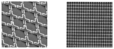
Figure 1.1: Experimental samples: square proximity-effect Pb/Cu/Pb Josephson Junction Arrays SEM’s image, with an array lattice space $a=10\mu m$ and distance between superconducting islands $d=1\mu m$ (the authors thank to Dr. H. Pastoriza and collaborators, Centro Atómico Bariloche, Argentina, for this picture.)

We study the dynamics of square Josephson junction array (JJA) with $L\times L$ superconducting nodes (see Fig.1.1) using the Resistively Shunted Junction (RSJ) model for the junctions [46, 47, 48, 49, 50]. The nodes are in the lattice sites ${\bf n}=(n_{x},n_{y})$ and their superconducting phases are $\theta({\bf n})$. Basically we have an XY model, therefore its Hamiltonian is the following:

$${\cal H}=-\sum_{\mu,{\bf n}}\frac{\Phi_{0}I_{0}}{2\pi}\cos[\theta({\bf n}+{\bf\mu})-\theta({\bf n})-A_{\mu}({\bf n})]\;.$$ (1.1)

Using this model, the current flowing in the junction between two superconducting nodes in the JJA is modeled as the sum of the Josephson supercurrent and the normal current:

$$I_{\mu}({\bf n})=I_{0}\sin\theta_{\mu}({\bf n})+\frac{\hbar}{2eR_{N}}\frac{d\theta_{\mu}({\bf n})}{dt}+\eta_{\mu}({\bf n},t)$$ (1.2)

being $I_{0}$ the critical current of the junction between the sites ${\bf n}$ and ${\bf n}+{\bf\mu}$, (${\bf\mu}={\bf\hat{x}},{\bf\hat{y}}$), $R_{N}$ the normal state resistance and

$$\theta_{\mu}({\bf n})=\theta({\bf n}+{\bf\mu})-\theta({\bf n})-A_{\mu}({\bf n})=\Delta_{\mu}\theta({\bf n})-A_{\mu}({\bf n})$$ (1.3)

the gauge invariant phase difference with

$$A_{\mu}({\bf n})=\frac{2\pi}{\Phi_{0}}\int_{{\bf n}a}^{({\bf n}+{\bf\mu})a}{\bf A}\cdot d{\bf l}.$$ (1.4)

The thermal noise fluctuations $\eta_{\mu}$ have correlations

$$\langle\eta_{\mu}({\bf n},t)\eta_{\mu^{\prime}}({\bf n^{\prime}},t^{\prime})\rangle=\frac{2kT}{R_{N}}\delta_{\mu,\mu^{\prime}}\delta_{{\bf n},{\bf n^{\prime}}}\delta(t-t^{\prime}).$$ (1.5)

In the presence of an external magnetic field $H$ we have

$$\Delta_{\mu}\times A_{\mu}({\bf n}) = A_{x}({\bf n})-A_{x}({\bf n}+{\bf y})+A_{y}({\bf n}+{\bf x})-A_{y}({\bf n})$$ (1.6)

$$= 2\pi f,$$

$f=Ha^{2}/\Phi_{0}$ and $a$ is the array lattice spacing. If the magnetic field is such that $f=1/L^{2}$ it corresponds to have one vortex in the sample, if $f=1/25$ we have an example of diluted vortex lattices, if $f=1/2$, there is half flux quantum per plaquette and the JJA correspond to the fully frustrated XY model.

We take periodic boundary conditions (PBC) in both directions in the presence of an external current ${\bf I}=I{\bf\hat{y}}$ [35] (See Appendix A). The vector potential is taken as

$$A_{\mu}({\bf n},t)=A_{\mu}^{0}({\bf n})-\alpha_{\mu}(t)$$ (1.7)

where in the Landau gauge $A^{0}_{x}({\bf n})=-2\pi fn_{y}$, $A^{0}_{y}({\bf n})=0$ and $\alpha_{\mu}(t)$ allows for total voltage fluctuations under periodic boundary conditions. In this gauge the PBC for the phases are [23, 25, 35]:

$$\theta(n_{x}+L,n_{y}) = \theta(n_{x},n_{y})$$

$$\theta(n_{x},n_{y}+L) = \theta(n_{x},n_{y})-2\pi fLn_{x}.$$ (1.8)

We also consider local conservation of current,

$$\Delta_{\mu}\cdot I_{\mu}({\bf n})=\sum_{\mu}I_{\mu}({\bf n})-I_{\mu}({\bf n}-{\bf\mu})=0.$$ (1.9)

After Eqs. (1.2,1.9) we obtain the following equations for the phases [23, 25, 35],

$$\frac{\hbar}{2eR_{N}}\Delta_{\mu}^{2}\frac{d\theta({\bf n})}{dt}=-\Delta_{\mu}\cdot[S_{\mu}({\bf n})+\eta_{\mu}({\bf n},t)]$$ (1.10)

where

$$S_{\mu}({\bf n})=I_{0}\sin[\Delta_{\mu}\theta({\bf n})-A_{\mu}^{0}({\bf n})-\alpha_{\mu}]\;,$$ (1.11)

and the discrete Laplacian is

$$\Delta^{2}_{\mu}f({\bf n}) = f({\bf n}+{\bf\hat{x}})+f({\bf n}-{\bf\hat{x}})+f({\bf n}+{\bf\hat{y}})+f({\bf n}-{\bf\hat{y}})$$ (1.12)

$$\;-4\,f({\bf n}).$$

The Laplacian can be inverted with the square lattice Green’s function $G_{{\bf n},{\bf n^{\prime}}}$:

$$\Delta^{2}_{\mu}G_{{\bf n},{\bf n^{\prime}}}=\delta_{{\bf n},{\bf n^{\prime}}}.$$ (1.13)

Since we take PBC (see Appendix A), the total current has to be fixed by:

$$I_{x} = \frac{1}{L^{2}}\left[\sum_{{\bf n}}I_{0}\sin\theta_{x}({\bf n})+\eta_{x}({\bf n},t)\right]+\frac{\hbar}{2eR_{N}}\frac{d\alpha_{x}}{dt}\;,$$

$$I_{y} = \frac{1}{L^{2}}\left[\sum_{{\bf n}}I_{0}\sin\theta_{y}({\bf n})+\eta_{y}({\bf n},t)\right]+\frac{\hbar}{2eR_{N}}\frac{d\alpha_{y}}{dt}\;,$$

These equations determine the dynamics of $\alpha_{\mu}(t)$ [35]. For the case of a current flowing in the $y$ direction we take $I_{x}=0$ and $I_{y}=I$ and for the case in which we apply a current $I$ at an angle $\phi$ with respect to the $[10]$ lattice direction, $I_{x}=I\cos\phi$ and $I_{y}=I\sin\phi.$ After Eqs. (1.10,1.13,LABEL:tot) we obtain the following set of dynamical equations [23, 25, 35],

$$\frac{d\theta({\bf n})}{dt} = -\sum_{\bf n^{\prime}}G_{{\bf n},{\bf n^{\prime}}}\Delta_{\mu}\cdot\left[S_{\mu}({\bf n^{\prime}})+\eta_{\mu}({\bf n^{\prime}},t)\right],$$ (1.15)

$$\frac{d\alpha_{\mu}}{dt} = I_{\mu}-\frac{1}{L^{2}}\sum_{{\bf n}}S_{\mu}({\bf n})+\eta_{\mu}({\bf n},t),$$ (1.16)

where we have normalized currents by $I_{0}$, time by $\tau_{J}=2eR_{N}I_{0}/\hbar$, and temperature by $I_{0}\Phi_{0}/2\pi k_{B}$.

1.2.2 Comparison with thin film with a periodic array of holes

Let us consider a superconducting thin film with a square array of holes, which act as pinning sites for vortices. There are $N_{p}=L^{2}$ pinning sites separated by a distance $a$. The current density in the superconducting film is given by the sum of the supercurrent and the normal current:

$${\bf J} = {\bf J}_{S}+{\bf J}_{N}$$

$${\bf J} = \frac{ie\hbar}{m^{*}}\left[\Psi^{*}{\bf D}\Psi-({\bf D}\Psi)^{*}\Psi\right]+\frac{\sigma\Phi_{0}}{2\pi c}\frac{\partial}{\partial t}\left(\nabla\theta-\frac{2\pi}{\Phi_{0}}{\bf A}\right),$$

with ${\bf D}=\nabla+i\frac{2\pi}{\Phi_{0}}{\bf A}$, $\Psi({\bf r})=|\Psi({\bf r})|\exp[i\theta({\bf r})]$ the superconducting order parameter and $\sigma$ the normal state conductivity. These equations are valid everywhere in the film except in the hole regions. If the number of vortices $N_{v}=BL^{2}a^{2}/\Phi_{0}$ is much smaller than the number of pinning sites $N_{p}$, all vortices will be centered in the holes in equilibrium. In this case we can assume that $|\Psi({\bf n})|\approx|\Psi_{0}|$ is homogeneous in the superconducting film. Therefore the dynamics is given by the superconducting phase $\theta({\bf r})$, corresponding to a London model in a sample with holes. After considering current conservation $\nabla\cdot{\bf J}=0,$ we obtain the London dynamical equations for the phases in this multiply connected geometry. Since $N_{v}\ll N_{p}$, we make the approximation of solving the equations in a discrete grid of spacing $a$. This means that we take as the relevant dynamical variables the phases $\theta({\bf r}_{\bf n})$ defined in the sites which are dual to the pinning sites. They represent the average superconducting phase in each superconducting square defined by four pinning sites. Therefore, we take the discretization ${\bf r}_{\bf n}=(n_{x}a,n_{y}a)=a{\bf n}$. [Pinning sites at centered at positions ${\bf r}_{\bf p}=(n_{x}+1/2,n_{y}+1/2)a$]. The derivatives in the supercurrent are discretized in a gauge-invariant way as

$$D_{\mu}\Psi({\bf r})\rightarrow\frac{1}{a}\left[\Psi({\bf n}+{\bf\mu})-e^{-i2\pi A_{\mu}({\bf n})/\Phi_{0}}\Psi({\bf n})\right].$$ (1.18)

After doing this, we obtain an equation analogous to (1.2). Now $I_{\mu}({\bf n})$ has to be interpreted as current density normalized by $J_{0}=2e\hbar|\Psi_{0}|^{2}/ma=\Phi_{0}/(8\pi^{2}\lambda^{2}a)$, time normalized by $\tau=c/(4\pi\sigma\lambda^{2})$, and the fraction of vortices is $f=N_{v}/N_{p}=Ba^{2}/\Phi_{0}$. This leads to a set of dynamical equations of the same form as Eqs.(1.15,1.16). Therefore, we expect that for $f\ll 1$ the model for a JJA also gives a good representation of the physics of a superconducting film with a square array of holes (meaning that effects of interstitial vortices are neglected for $N_{v}\ll N_{p}$). In other words, we expect that for a low density of vortices the specific shape of the periodic pinning potential (being either an egg-carton or an array of holes) will not be physically relevant.

1.2.3 Quantities calculated and simulation parameters

The Langevin dynamical equations (1.15,1.16) are solved with a second order Runge-Kutta-Helfand-Greenside algorithm with time step $\Delta t=(0.05-0.1)\tau_{J}$. The discrete periodic Laplacian is inverted with a fast Fourier + tridiagonalization algorithm (see the Appendix B for a detail of the algorithm used).

The main physical quantities calculated are the following:

(i) Transverse superconducting coherence: We obtain the helicity modulus $\Upsilon_{x}$ in the direction transverse to the current as

$$\Upsilon_{x} = \frac{1}{L^{2}}\left\langle\sum_{{\bf n}}\cos\theta_{x}({\bf n})\right\rangle-\frac{1}{TL^{4}}\left\{\left\langle\left[\sum_{{\bf n}}\sin\theta_{x}({\bf n})\right]^{2}\right\rangle\right.$$

$$\left.-\left\langle\left[\sum_{{\bf n}}\sin\theta_{x}({\bf n})\right]\right\rangle^{2}\right\}$$

Whenever we calculate the helicity modulus along $x$, we enforce strict periodicity in $\theta$ by fixing $\alpha_{x}(t)=0$ (see Appendix A).

(ii)Transport: We calculate the transport response of the JJA from the time average of the total voltage as

$$V_{x} = \langle v_{x}(t)\rangle=\langle d\alpha_{x}(t)/dt\rangle$$

$$V_{y} = \langle v_{y}(t)\rangle=\langle d\alpha_{y}(t)/dt\rangle$$ (1.19)

with voltages normalized by $R_{N}I_{0}$.

Figure 1.2: Left: schematic representation of a square Josephson junction array, the crosses indicate Josephson junctions (JJ), with a rotated applied external current. Right: definition of angles with respect to the $x$ and $y$ axis of the array. The vector of applied current ${\bf I}=(I_{x},I_{y})$ forms an angle $\phi$ respect to the $x$-axis. The vector of electric field ${\bf E}=(V_{x},V_{y})$ forms an angle $\theta_{v}$ with respect to the $x$-axis and an angle $\theta_{t}$ with respect to the current ${\bf I}$.

(iii) Vortex structure: We obtain the vorticity at the plaquette ${\bf\tilde{n}}=(n_{x}+1/2,n_{y}+1/2)$ (associated to the site ${\bf n}$) as [51]:

$$b({\bf\tilde{n}})=-\Delta_{\mu}\times{\rm nint}[\theta_{\mu}({\bf n})/2\pi]$$ (1.20)

with ${\rm nint}[x]$ the nearest integer of $x$. We calculate the average vortex structure factor as

$$S({\bf k})=\left\langle\left|\frac{1}{L^{2}}\sum_{\bf\tilde{n}}b({\bf\tilde{n}})\exp(i{\bf k}\cdot{\bf\tilde{n}})\right|^{2}\right\rangle.$$ (1.21)

Analyzing above properties we study JJA under different magnetic fields applied. (a) Diluted vortex lattices corresponding to $f=1/25$. (b) A single vortex in the array, $f=1/L^{2}$. (c) And fully frustrated JJA, corresponding to have half flux quantum per plaquette, i.e. $f=1/2$. We consider square networks of $L\times L$ junctions, with $L=8,16,24,32,48,64,128$ or $L=50,100,150$. We apply dc currents in different directions: (i) $I$ flowing in the $y$ direction or (ii) $I$ at an angle $\phi$ with respect to the $[10]$ lattice direction,

$$I_{x} = I\cos\phi$$

$$I_{y} = I\sin\phi.$$ (1.22)

We define the longitudinal voltage as the voltage in the direction of the applied current,

$$V_{l}=V_{x}\cos\phi+V_{y}\sin\phi,$$ (1.23)

and the transverse voltage

$$V_{t}=-V_{x}\sin\phi+V_{y}\cos\phi.$$ (1.24)

From the voltage response, we define the transverse angle as

$$\tan\theta_{t}=V_{t}/V_{l}$$ (1.25)

and the voltage angle as

$$\tan\theta_{v}=V_{y}/V_{x},$$ (1.26)

i.e. $\theta_{t}=\theta_{v}-\phi$, see Fig. 1.2. When the vortices move in the direction perpendicular to the current, there is no transverse voltage, therefore $\theta_{t}=0$ and $\theta_{v}=\phi$. The case with a dc current applied in the $y$ direction, ${\bf I}=I{\bf\hat{y}}$ ($\phi=\pi/2$), will be the more extensively used in this review.

1.3 DILUTED VORTEX LATTICE DYNAMICS

In this section we show the study of JJA with a low magnetic field corresponding to $f=1/25$, diluted vortex lattices, for different system sizes of $L\times L$ junctions, with $L=50,100,150$. Most of the results are for $L=100$, except when it is explicitly specified, and for $N_{t}=10^{5}$ iterations after a transient of $N_{t}/2$ iterations.

1.3.1 Transition near equilibrium

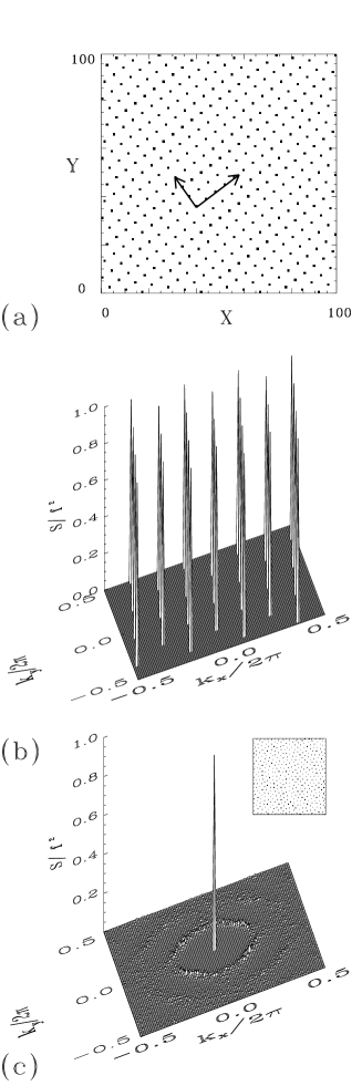
Figure 1.3: Vortex configuration for a low current $I=0.01\ll I_{c}(0)$ and a low temperature, $T=0.01<T_{M}$: (a) tilted square vortex lattice, oriented in the $[4a,3a]$ direction and (b) corresponding structure factor $S({\bf k})$. At high temperature, $T=0.05\gtrsim T_{M}$: (c) disordered vortex array. Inset: vortex liquid-like structure factor.

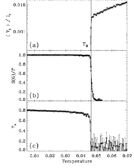
Figure 1.4: For low current $I\ll I_{c}(0)$, $I=0.01$: (a) $<V_{y}>/I_{y}$ vs. $T$, (b) $S({\bf G_{1}})$ $(\diamond)$ and $S({\bf G_{2}})$ $(\star)$ vs. $T$, (c) $\Upsilon_{x}$ vs. $T$.

The ground state vortex configuration for $f=1/25$ is a tilted square-like vortex lattice (VL) [52], see Fig.1.3(a). We find that this state is stable for low currents and low temperatures (in fact, the structure of Fig.1.3(a) corresponds to $I=0.01$ and $T=0.01$). The lattice is oriented in the $[4a,3a]$ direction and commensurated with the underlying periodic pinning potential of the square JJA. The structure factor $S({\bf k})$ has the corresponding Bragg peaks at wavevectors ${\bf G}$ in the reciprocal space, as can be seen in Fig.1.3(b). When the temperature is increased, the VL tends to disorder and above the melting temperature $T_{M}$ a random vortex array with a liquid-like structure factor is obtained, Figs.1.3(c) and inset.

We find a single equilibrium phase transition ($I=0$) at $T_{M}\approx 0.050\pm 0.003$, which is in agreement with the melting temperature obtained by Franz and Teitel[14] and Hattel and Wheatley[15] for $f\gtrsim 1/30$.

We now apply a very low current, $I=0.01$, in order to study the near-equilibrium transport response simultaneously with other quantities like structure factor and helicity modulus. We find a phase transition at a temperature $T_{M}(I)\approx 0.046\pm 0.001$, which is slightly lower than the equilibrium transition. In Fig.1.4(a) we see that there is a large jump in the resistance $R=V/I$ at $T_{c}$, in good agreement with the first-order nature of the equilibrium transition [14]. The onset of resistivity is a signature of a

Figure 1.5: Zero temperature $IV$ curve. There is a critical current $I_{c}(0)=0.114\pm 0.002$.

depinning transition in the direction of the drive. This occurs simultaneously with a melting of the vortex lattice, corresponding to the vanishing of Bragg peaks, as shown in Fig.1.4(b) for the two first reciprocal lattice vectors ${\bf G_{1}}=\frac{2\pi}{a}(-4/25,-3/25)$ and ${\bf G_{2}}=\frac{2\pi}{a}(-3/25,4/25)$. In the direction of the current drive the helicity modulus is ill-defined since total phase fluctuations are allowed (see Appendix A). However, in the perpendicular direction to the drive the helicity modulus $\Upsilon_{x}$ can be calculated, and it is a measure of the transverse superconducting coherence. As we can see in Fig.1.4(c), transverse superconductivity also vanishes at $T_{M}(I)$. Above $T_{M}$, we find that the $\Upsilon_{x}(T)$ has large fluctuations around zero.

Figure 1.6: $IV$ curves for different temperatures. Linear scale, crossing point at $I^{*}=0.165$. Inset: Log-log plot of $R=V/I$ vs. $I$ for the same temperatures.

1.3.2 Transport properties

Let us now study the transport properties for larger currents. We calculate the current-voltage (IV) characteristics for different temperatures as well as the dc resistance $R=V/I$ as a function of temperature for finite currents.

The zero temperature IV curve has a critical current, $I_{c}(0)=0.114\pm 0.002$, see Fig.1.5, which corresponds to the single vortex depinning current in square JJA [4], with the typical square root depence at the onset. Similar behavior has been reported for zero temperature IV curves for low values of $f$ [53, 54]. Above $I_{c}(0)$ there is an almost linear increase of voltage, corresponding to a “flux flow” regime, where there is a fastly moving VL. The structure factor of the $T=0$ moving VL is the same as the corresponding one of the pinned VL [Fig.1.3(a)]. The presence of periodic boundary conditions in our case prevents the occurrence of random or chaotic vortex motion near the critical current, as reported in early simulations with free boundary conditions [46, 47]. In what follows we will restrict our analysis for currents $I<0.4$, where the collective behavior of the VL is the dominant physics (at $I\sim 1$ there is a sharp increase of voltage when all the junctions become normal, and $V\sim R_{N}I$ for $I\gg 1$).

Figure 1.7: $<V_{y}>/I_{y}$ vs temperature curves for different dc currents ($I_{y}$).

The IV curves for finite temperatures are shown in Fig.1.6. For temperatures below $T_{M}$ there is a nonlinear sharp rise in voltage which defines the apparent critical current $I_{c}(T)$. For example, we can obtain this $I_{c}(T)$ with a voltage criterion, which we choose as $V<\frac{1}{N_{t}\Delta t}=10^{-4}$. In this case, we find that $I_{c}(T)$ decreases with $T$, vanishing at $T_{M}$. It is interesting to point out that all the IV curves for different temperatures have a crossing point at $I^{*}=0.165$, see Fig.1.6. A crossing in the IVs has also been reported in experiments in amorphous thin films [55]. For temperatures $T>T_{M}$ the IV curves tend to linear resistivity for low currents. This is shown in the inset of Fig.1.6 in a log-log plot of $R(I)=V/I$ vs $I$, where we see that $R(I)$ tends to a low current finite value for $T>T_{M}$, while it has a strong nonlinear decrease for $T<T_{M}$.

Let us now study the dc resistance $R=V/I$ as a function of temperature for a given applied current in the $y$-direction (Fig.1.7). We start with the perfectly ordered VL as an initial condition at $T=0$ and then we slowly increase the temperature, keeping $I$ constant. For currents below the $T=0$ critical current, $I<I_{c}(0)$, the dc resistance is negligibly small at low $T$, and it has a steep increase at a depinning temperature $T_{p}(I)$, corresponding to the onset of vortex motion. The depinning temperature decreases for increasing currents, and the values of $T_{p}(I)$ are coincident with the apparent critical currents $I_{c}(T)$ obtained from the IV curves. For currents higher than $I_{c}(0)$, there is always a large and finite voltage for any temperature. If $I_{c}(0)<I<I^{*}$, the $R(I)$ increases slightly with $T$ tending to a constant value for large $T$, while for $I>I^{*}$ the $R(I)$ decreases with $T$.

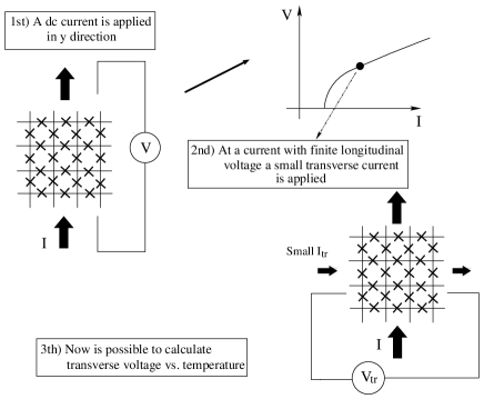
Figure 1.8: How to get “schematically” the transverse temperature depinning.

1.3.3 Transverse depinning

What is its response to a small current in the transverse direction when the driven vortex lattice is moving? Is the vortex lattice still pinned in the transverse direction? Is there a transverse critical current for a moving VL? The idea of a transverse depinning current was introduced by Giamarchi and Le Doussal in Ref.[30] for moving vortex systems with random pinning at zero temperature. The possibility of such a critical current was later questioned by Balents, Marchetti and Radzihovsky [31], where it was shown that this is not true for any finite temperature in random pinning; however a strong nonlinear increase of the transverse voltage was predicted at an “effective” transverse critical current. In the case of periodic pinning it is more clear that a transverse critical current will exist at $T=0$ since it is a commensurability effect. This has been found in the $T=0$ simulation work of Reichhardt et al [18]. It is also possible that this transverse critical current will still be non-zero at $T\not=0$ in periodic pinning. In fact, we have found in our previous work [23] that there is a thermal transverse depinning in a periodic system, and we will now analyze this behavior in detail.

Figure 1.9: Transverse depinnig temperature determinations. With a small transverse current applied, $I_{x}=0.01$, and $I_{y}=0.16$, $<V_{tr}/I_{tr}>$ vs $T$. Inset: $Tr-IV$ curve and $<V_{y}>$ vs $I_{tr}/I_{y}$ at $T=0$ and high longitudinal current, $I_{y}=0.16$.

Figure 1.10: Transverse $IV$ curves for different temperatures: (a) low current $I_{y}<I_{c}(0)$, $I_{y}=0.06$, (b) high current $I_{y}>I_{c}(0)$, $I_{y}=0.16$.

First, a high longitudinal current $I>I_{c}(0)$ is applied at zero temperature. Then, a current $I_{tr}$ is applied in the transverse direction (see Fig.1.8 scheme). In this way, a transverse current-voltage characteristics can be obtained for each $I$. This is shown in the inset of Fig.1.9 for $I=0.16$. We clearly see that there is a finite transverse critical current $I_{c,tr}\approx 0.12$, which is of the order of the single vortex pinning barrier. We also show in the inset of Fig.1.9, how the longitudinal voltage $V$ changes when the transverse current is varied. For $I_{tr}<I_{c,tr}$ the longitudinal voltage $V$ is almost constant. At $I_{c,tr}$ there is a fast decay of $V$. When $I_{tr}=I$ we also have $V=V_{tr}$ as expected for a drive at a degree of $\pi/4$. Later, for $I_{tr}>I$ the vortex lattice becomes pinned in the other direction, since now the directions of “longitudinal” and “transverse” current are interchanged.

Another possible measurement is to study thermal transverse depinning. In this case, we start with a longitudinal current $I$, then a small transverse current is applied, $I_{tr}\ll I_{c,tr}$, and the temperature is slowly increased. In this way, we can measure a transverse resistance $R_{tr}=V_{tr}/I_{tr}$ like it was showed schematically in Fig.1.8. In Fig.1.9 we plot this result for $I=0.16$ and $I_{tr}=0.01$. We find that for finite low temperatures $R_{tr}$ is negligibly small within our numerical accuracy and it has a clear onset at a transverse critical temperature $T_{tr}$.

Let us now see how these results depend on the longitudinal current $I$ and temperature $T$. We have calculated the transverse IV (Tr-IV) curves for different $I$ and $T$. In Fig.1.10(a) we show the Tr-IV curves for $I=0.06$ (low current regime) and in Fig.1.10(b) for $I=0.16$ (high current regime). In both cases, there is a clear change of behavior in the Tr-IV curves when going through a characteristic transverse critical temperature $T_{tr}(I)$. For low temperatures there is a transverse critical current which tends to vanish when $T$ aproachs $T_{tr}(I)$ from below. In contrast, for $T>T_{tr}$ there is a linear resistivity behaviour.

The transverse resistivity $R_{tr}=V_{tr}/I_{tr}$ as a function of temperature was calculated for different longitudinal currents (Fig.1.11). In all cases there is an onset of transverse response at a given temperature $T_{tr}(I)$. At low currents, $I<I_{c}(0)$, the transverse depinning temperatures are almost constant, $T_{tr}\sim 0.02$ tending to increase slowly with $I$, see Fig.1.11. On the other hand, for $I>I_{c}(0)$ the transverse depinning temperatures increase clearly with $I$, see the inset in Fig.1.11.

1.3.4 Non-equilibrium regimes

We will now study the different non-equilibrium regimes of vortex driven lattices and characterize their possible dynamical transitions. The approach we will follow in this subsection is to have a fixed current applied in the system and vary the temperature. In this way, we look for the possible transitions as a function of $T$ in a similar way as was done near equilibrium in Sec. 1.3.1.

A few similar studies were done previously in related systems. In Ref. [34] the melting transition of a moving vortex lattice in the three dimensional XY model was studied in this way. In this work a first order transition was found as a function of temperature in a strongly driven vortex lattice. In Ref. [50] a current driven two dimensional JJA at zero field was studied. The possibility of a transition as a function of temperature for finite currents below the critical current was analyzed in this case.

Figure 1.11: $V_{tr}/I_{tr}$ vs $T$ curves for different dc currents applied in the $y$ direction and small transverse current applied, $I_{x}=0.01$: for low current $I_{y}<I_{c}(0)$. Inset: for high current $I_{y}>I_{c}(0)$.

In the following, we will separate our study in three ranges of current: low currents, $I<0.04$ , intermediate currents $0.04<I<I_{c}(0)$ , and high currents $I>I_{c}(0)$ .

Figure 1.12: For low current $I<I_{c}(0)$, $I=0.03$: (a) $<V_{y}>/I_{y}$ vs. $T$, (b) $S({\bf G_{1}})$ $(\diamond)$ and $S({\bf G_{2}})$ $(\star)$ vs. $T$, inset: size effect in $S({\bf G_{1}})$, (c) $\Upsilon_{x}$ vs. $T$.

Low currents

We show the results for a low current in Fig.1.12 for $I=0.03$. The longitudinal dc response, $V/I$, is negligibly small at low $T$ and later it has a sharp increase of two orders of magnitude: this defines the depinning temperature, $T_{p}$ [Fig.1.12(a)]. At higher temperatures, $T>T_{p}$, the resistance is weakly $T$-dependent.

Below $T_{p}$ the vortex lattice is pinned and its structure is similar to the ground state: a vortex lattice commensurate with the underlying square array and tilted in the $[4a,3a]$ direction. Above $T_{p}$ the vortex lattice is moving and it has an anisotropic structural order. If we analyze the structure factor in two different reciprocal lattice directions $S(G_{1})$ and $S(G_{2})$, we can see this clearly (Fig.1.12(b)). Below $T_{p}$ the VL structure is isotropic and $S(G_{1})=S(G_{2})$. Right above $T_{p}$ the height of the peaks decreases with temperature, and the structure of the depinned VL is clearly anisotropic, $S(G_{1})\not=S(G_{2})$. Finally, at a melting temperature $T_{M}$ the peaks vanish, and the vortex lattice melts into a vortex liquid. In Fig.1.12(b) inset we compare the behavior of the Bragg peaks for two system sizes $L=50,100$. We see that the $S(G_{1,2})$ are size independent below $T_{p}$ as it should be expected for a pinned phase [14].

The helicity modulus in the direction perpendicular to the current, $\Upsilon_{x}$, decreases very slowly for $T<T_{p}$. Above $T_{p}$, $\Upsilon_{x}$ has a faster decay with important fluctuations and tends to vanish at $T_{M}$. For $T>T_{M}$, $\Upsilon_{x}$ oscillates around zero. Therefore, for a small finite current the depinning and melting transitions become separated with $T_{p}<T_{M}$.

Figure 1.13: For $I<I_{c}(0)$, $I=0.06$: (a) $<V_{tr}>/I_{tr}$ vs. $T$, (b) $<V_{y}>/I_{y}$ vs. $T$, (c) $S({\bf G_{1}})$ $(\diamond)$ and $S({\bf G_{2}})$ $(\star)$ vs. $T$, (d) $\Upsilon_{x}$ vs. $T$.

Figure 1.14: For intermediate current $I<I_{c}(0)$, $I=0.06$: size effect in $S({\bf G_{1}})$.

Intermediate currents

At intermediate currents, $0.04<I<I_{c}(0)$, a new transition appears: the transverse depinning of the moving vortex lattice. As discussed in Sec. 1.3.3, one can measure transverse depinning by applying a small transverse current while the VL is driven with a fixed longitudinal current. This is shown in Fig. 1.13(a) for the case of $I=0.06$ and a small transverse current, $I_{tr}=0.01$. We see that there is an onset of transverse voltage at $T_{tr}=0.019$. We can also see that this transverse depinning temperature is above the depinning temperature $T_{p}$ for longitudinal resistance [Fig.1.13(b), $T_{p}=0.013$], and below the melting temperature $T_{M}$ for the vanishing of the Bragg peaks [Fig.1.13(c), $T_{M}=0.037$]. Therefore, this transition occurs at an intermediate temperature between the depinning and the melting transitions, $T_{p}<T_{tr}<T_{M}$. We also show in Fig.1.13(d) that the helicity modulus begins to fall down slowly at $T_{tr}$, while for $T_{tr}<T<T_{M}$ it has strong fluctuations, being difficult to interpret its behavior in this case.

One can see that the intensity of the Bragg peaks has a greater dependence with size for $T_{tr}<T<T_{M}$ when compared with the $T_{p}<T<T_{tr}$ regime in Fig.1.14. For large temperatures $T>T_{M}$, in the liquid phase, the value of $S(G_{1,2})$ in general is strongly size dependent, since it should go as $L^{-2}$ [14]. On the other hand, for $T_{p}<T<T_{M}$ we find that the intensity of the Bragg peaks is weakly dependent on system size. The clear change of behavior of the size dependence gives a good criterion to determine $T_{M}$ (Fig.1.14).

It is interesting to study in more detail the behavior of the structure factor through all these transitions. In Fig.1.15 we show examples of the structure factor $S({\bf k})$ at temperatures in the different regimes. In the pinned phase, the $S({\bf k})$ is nearly the same as in the ground state with delta-like Bragg peaks, see Fig.1.15(a). For the moving VL, we can see that there is less anisotropy in the transversely pinned regime $T_{p}<T<T_{tr}$ [Fig.1.15(b)] than in the floating regime $T_{tr}<T<T_{M}$ [Fig.1.15(c-d)]. Moreover, near $T_{M}$ the VL structure becomes strongly anisotropic, with the peak at ${\bf G}_{1}$ much larger than the peak at ${\bf G}_{2}$ (see Fig.1.15(d) and Fig.1.14).

The anisotropy of the Bragg peaks of the moving VL (in the regimes at $T_{p}<T<T_{M}$) has two characteristics: (i) the width of the peaks increases with $T$ in the direction of the applied current (the direction perpendicular to the vortex motion), and (ii) the height of the peaks decreases in the direction of vortex motion. This can be observed in the sequence of structure factors shown in Fig.1.15.

Figure 1.15: Intensity plot of the structure factor $S({\bf G})$ at $I<I_{c}(0)$, $I=0.06$ for different temperatures: (a) $T<T_{p}$, $T=0.006$, (b) $T_{p}<T<T_{tr}$, $T=0.0185$, (c) $T_{tr}<T<T_{M}$, $T=0.024$, (d) $T\leq T_{M}$, $T=0.035$.

Figure 1.16: For high current $I>I_{c}(0)$, $I=0.16$: (a) $<V_{tr}>/I_{tr}$ vs. $T$, (b) $S({\bf G_{1}})$ $(\diamond)$ and $S({\bf G_{2}})$ $(\star)$ vs. $T$, (c) $\Upsilon_{x}$ vs. $T$.

High currents

In the case of currents larger than $I_{c}(0)$, the vortex lattice is already depinned at $T=0$. As we have seen in Sec. 1.3.3, this zero-temperature moving VL has a finite transverse critical current, and therefore it is pinned in the transverse direction. When we slowly increase temperature from this state, we find that the transverse resistive response is negligible for finite low temperatures. At a temperature $T_{tr}$ there is a jump to a finite transverse resistance $R_{tr}=V_{tr}/I_{tr}$. For example, this is shown for $I=0.16$ with a small transverse current, $I_{x}=0.01$ in Fig.1.16(a). The vortex lattice has an anisotropic structural order for all temperatures, i.e, $S({\bf G_{1}})\neq S({\bf G_{2}})$, and the height of the Bragg peaks vanishes at $T_{M}$, Fig.1.16(b). The transverse helicity modulus $({\Upsilon_{x}})$ is almost constant for low temperatures and starts to decrease at $T_{tr}$ presenting strong fluctuations for $T>T_{tr}$ , Fig1.16(c). In Fig.1.17 we show $S({\bf G_{2}})$ for different sizes, $L=50,100$, and we see that $T_{M}$ is size independent. Similar behaviour is found for $S({\bf G_{1}})$.

The analysis of the heights of the peaks in $S({\bf k})$ as a function of system size $L$ is a good indicator of the translational correlations in the system. This dependence is well known for two dimensional lattices [14]. For a pinned solid $S({\bf G})\sim 1$, for a floating solid, $S({\bf G})\sim L^{-\eta_{G}(I,T)}$ with $0<{\eta_{G}(I,T)}<2$, being this dependence a signature of quasi-long range order, and for a normal liquid $S({\bf G})\sim L^{-2}$. To assure the existence of algebraic translational

Figure 1.17: For high current $I>I_{c}(0)$, $I=0.16$: size effect in $S({\bf G_{2}})$ vs. $T$.

Figure 1.18: Finite size analysis and power law fit of $S({\bf G})\sim L^{-\eta_{G}}(I,T)$ for a moving vortex lattice at $I>I_{c}(0)$, $I=0.16.$ We obtain: (a) for $T<T_{tr}$, $T=0.02$, $\eta_{G_{1}}=0.023$ $(\star)$ and $\eta_{G_{2}}=0.013$, $(\triangle)$, (b) for $T_{tr}<T<T_{M}$, $T=0.035$, $\eta_{G_{1}}=0.471$ $(\star)$ and $\eta_{G_{2}}=0.34$ $(\triangle).$ Inset: at same $I$, $\eta(I,{\bf G})$ vs $T$, for ${\bf G_{1}}$and ${\bf G_{2}}$.

correlations, we have done this scaling study for currents $0.02<I<0.2$ and different temperatures for system sizes of $L=50,100,150$. For the cases corresponding to the pinned regime ($T<T_{p}$) we found $\eta_{G}\approx 0$, as expected. In the transversely pinned regime, we show a case in Fig.1.18(a), we find a power law fitting with very small values of ${\eta_{G}}(I,T)$. In the floating regime, we find larger values of $\eta_{G}$, we show a case in Fig.1.18(b). In all the cases we have obtained that $0<{\eta_{G}}(I,T)<2$ for $T_{p}<T<T_{M}$. Therefore, this finite size analysis shows the existence of quasi-long range order in the moving VL. Also, we find that ${\eta_{G_{1}}}>{\eta_{G_{2}}}$ for all currents and temperatures. The power-law exponent ${\eta_{G}}$ can be studied at a constant current, as a function of temperature. This is shown in the inset of Fig.1.18(b), for $I=0.16$ and different reciprocal lattice vectors. The exponent ${\eta}$ is finite for the complete temperature range. For $T<T_{tr}$ it has a small value $\eta_{G}\approx 0.01$. It has a fast increase near $T_{tr}$, where there is also a clear difference between ${\eta_{G_{1}}}$ and ${\eta_{G_{2}}}$. Finally, it reaches a value of ${\eta=2}$ near $T=T_{M}$.

1.3.5 Orientational pinning effects

A very interesting characterization of the different regimes showed in the precedent subsection can be obtained by studying the effects of varying current direction [24, 56, 57]. We apply a current $I$ at an angle $\phi$ with respect to the $[10]$ lattice direction, $I_{x}=I\cos\phi,I_{y}=I\sin\phi$ (see Sec. 1.2.3). We study the voltage response when varying the orientation $\phi$ of the drive while keeping fixed the amplitude $I$ of the current. In the parametric curves of $V_{y}(\phi)$ vs. $V_{x}(\phi)$ can we analyze the breaking of rotational symmetry in the different regimes of $I$ and $T$. In the case of rotational symmetry this kind of plot should give a perfect circle. However, the square symmetry of the Josephson lattice will show up in the shape of the curves. In what follows we start studying the motion of single vortices in JJA (1), to show later the breaking of rotational invariance in diluted vortex lattices (2) and how this effect could be used to characterized the dynamical regimes described previously. The first case of a single vortex is studied before for its simplicity. In order to understand the phenomenon of breaking of rotational symmetry is better to begin without including the collective effects of vortex lattices. In addition, experimental evidences were found simultaneously for Dr. H. Pastoriza and collaborators [24] for this case. And very nice agreement between numerical and experimental results was found.

Breaking of rotational invariance in JJA with a single vortex

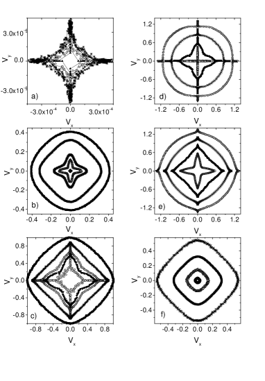
Figure 1.19: Simulation results of the parametric curves $V_{y}(\phi)$ vs. $V_{x}(\phi)$. (a) $I=0.2$, for (going outwards from the center) $T=0$, $T=0.01$ and $T=0.05$; (b) $I=0.6$ for $T=0.3$, $T=0.5$, $T=0.6$, $T=1.0$ and $T=1.4$; (c) $I=1.2$ for $T=0$, $T=0.05$, $T=0.1$, $T=0.3$ and $T=1.0$. (d) $T=0.05$ for (going outwards from the center) $I=1.0$, $I=1.2$, $I=1.4$ and $I=1.6$; (e) $T=0.2$ for $I=1.0$, $I=1.2$, $I=1.4$ and $I=1.6$; (f) $T=1.0$ for $I=0.2$, $I=0.4$, $I=0.6$ and $I=0.8$.

The square lattice has two directions of maximum symmetry: the [10] and the [11] directions (and the ones obtained from them by $\pi/2$ rotations), which correspond to the directions of reflection symmetry. When the current bias is in the [10] direction, the angle of the current is $\phi=0$, and we call it a “parallel” bias. When the current bias is in the [11] direction, the angle of the current is $\phi=\pi/4=45^{o}$, and we call it a “diagonal” bias (see squeme in Fig. 1.2).

In the case of the parallel bias we find that the transverse voltage is zero (in agreement with the reflection symmetry), see details in Ref. [24]. This corresponds to vortex motion in the direction perpendicular to the current ($\theta_{t}=0$). A perfect agreement with experimental results was found [24].

In the IV curve for the longitudinal voltage we find numerically a critical current corresponding to the single vortex depinning $I_{c}^{[10]}=0.1$ [4, 24]. In the case of the perfect diagonal bias, which is only attainable in the numerical model, we obtain similar results as in the parallel bias case. The transverse voltage is zero and therefore the vortex moves perpendicular to the current ($\theta_{t}=0$). In agreement with the prediction of Halsey [58], the numerical IV curve for $V_{l}$ has a critical current of $I_{c}^{[11]}=\sqrt{2}I_{c}^{[10]}=0.1414$. The onset of the resistive regime is also multiplied by a factor of $\sqrt{2}$.

For orientations different than the symmetry directions, we always find a finite transverse voltage (as well as was found in experiments [24]). In order to see this, we study the voltage response when varying the orientation $\phi$ of the drive while keeping fixed the amplitude $I$ of the current. If we analyze the transverse angle $\theta_{t}=\arctan({V_{t}}/{V_{l}})$ as a function of the angle of the current $\phi$ we observe that $\theta_{t}$ vanishes only in the maximum symmetry directions corresponding to angles $\phi=0,\pm 45^{o},\pm 90^{o},\dots$. Furthermore, we see that for orientations near $\phi=0$, the transverse angle basically follows the current angle: $\theta_{t}\approx-\phi$. This is an indication that vortex motion is pinned in the lattice direction [10], since $V_{y}\approx 0$, meaning that the voltage angle is $\theta_{v}\approx 0$. Whenever the voltage response is insensitive to small changes in the orientation of the current, we will call this phenomenon orientational pinning. On the other hand, near $\phi=45^{o}$ the transverse angle changes rapidly.

A more direct evidence of the breaking of rotational symmetry can be seen in the parametric curves of $V_{y}(\phi)$ vs. $V_{x}(\phi)$. In Fig. 1.19 we plot the values obtained for the voltages $V_{y}$ and $V_{x}$ when varying the orientational angle $\phi$ for different values of the current amplitude $I$ and the temperature. In the case of rotational symmetry we should have a perfect circle. In the set of plots of Fig. 1.19(a-c), the current amplitude is fixed and the temperature is varied. In Fig. 1.19(a) we have $I=0.2$, near the onset of single vortex motion in the regime. In this case most of the points are either on the axis $V_{x}=0$ or on the axis $V_{y}=0$, indicating strong orientational pinning in the lattice directions [10] or [01]. When increasing $T$ the orientational pinning decreases and the length of the “horns” in the $x$ and $y$ axis decreases. Fig. 1.19(b) corresponds to $I=0.6$ , when the vortex is moving fast. In this case the horns have disappeared and orientational pinning is lost. However, the breaking of rotational symmetry is still present in the star-shaped curves that we find at low $T$. The dip at $45^{0}$ in the stars are because in this direction the voltages are minimum, since the critical current is maximum in this case, $I_{c}^{[11]}=0.1\sqrt{2}$. When increasing the temperature, the stars tend to the circular shape of rotational invariance. Above the onset of the resistive regime the “horned” curves reappear. In this case the orientational pinning corresponds to the locking of ohmic dissipation in the junctions in one of the lattice directions, either [10] or [01]. Once again, when increasing $T$ the horned structure shrinks, and the curves evolve continuously from square shapes to circular shapes.

The variation with current of the rotational parametric curves for a fixed temperature is shown in the numerical results of Figs. 1.19(d-f). At a low temperature, $T=0.05$ we clearly see the horned structure of the curves for almost all the currents and even for large currents the circular curves have “horns”, see Fig. 1.19(d). At an intermediate temperature, $T=0.2$, there are still some signatures of the orientational pinning [Fig. 1.19(e)], while for $T=1.2$ all the curves are smooth and rounded with a slightly square shape [Fig. 1.19(f)].

Transverse voltage near the [1,1] direction

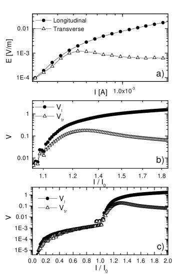
Figure 1.20: (a) Experimental results of longitudinal and transverse voltage for a current near the [11] direction, $\phi=45^{o}\pm 5$ at $T=1.25$ K. (b) Longitudinal and transverse voltage obtained numerically for $\phi=40^{o}$ at $T=0.02\,\hbar I_{0}/2ek_{B}$. (c) Idem (b) for an extended current range.

In Fig. 1.20(a) we show experimental voltage-current characteristics for an array of $100\times 1000$ junctions at a low temperature $T=1.25K$ and at a low magnetic field (results from Dr. Hernan Pastoriza’s Group, Argentina). The current is applied nominally in the [11] direction, but a small misalignment is possible in the setup of electrical contacts, therefore $\phi=45^{o}\pm 5^{o}$. We see that for low currents there is a very large value of the transverse voltage $V_{t}$, which is nearly of the same magnitude as the longitudinal voltage $V_{l}$. The transverse voltage is maximum at a characteristic current $I_{m}$. Above $I_{m}$, $V_{t}$ decreases with increasing current while $V_{l}$ increases. It is remarkable that these results are very different from the IV curve obtained numerically, where $V_{t}=0$ at $\phi=45^{o}$. However, if we assume a misalignment of a few degrees with respect to the [11] direction we can reproduce the experimental results. In Fig. 1.20(b) we show the IV curves obtained numerically for $\phi=40^{o}$ and $T=0.02$. We see that for low currents $V_{t}$ is close to $V_{l}$: $V_{t}\lesssim V_{l}$, similar to the experiment, and later $V_{t}$ has a maximum at a current $I_{m}\approx 1/\cos\phi\approx 1.3$. This corresponds to the current for which the junctions in the $x$-direction become critical ($I_{x}=1$). The highest transverse voltage can be obtained for orientations near $\phi=45^{o}$ as we explained before.

Therefore a slight misalignment of the array from the [11] direction is useful for studying both experimentally and numerically the behavior of the transverse voltage as a function of current and temperature.

Transverse voltage near the [1,1] direction in disordered JJA

Before we studied the breaking of rotational invariance in square JJA[24] at finite temperatures analyzing transport properties and we obtained that the transverse voltage vanishes only in the directions of maximum symmetry of the square lattice: the [10] and [01] direction (parallel bias) and the [11] direction (diagonal bias). For diagonal bias this result is highly unstable against small variations of the angle of the applied current, leading to a rapid change from zero transverse voltage to a large transverse voltage within a few degrees. Now we will show that a small amount of disorder induces finite transverse voltage in square JJA with a perfect diagonal bias. The transverse voltage as a function of current presents a peak which does not depend strongly with disorder for moderate disorder strength. This result is experimentally relevant since samples always could present a small amount of disorder due to tiny fabrication defects in addition to a possible misalignment in the setup of electrical contacts.

Figure 1.21: Numerical IV characteristics in a system of $32\times 32$ junctions with diagonal bias, at $T=0.02$,and $5$% of disorder compared with transverse voltage without disorder. Inset: transverse voltage peak for $5$%, $10$% and $15$% of disorder.

We simulate an square JJA with disorder in the critical currents using the RSJ model introduced before in Sec. 1.2.1. The modification to the current flowing in the junction between two superconducting islands is the following

$$I_{\mu}({\bf n})=g_{\mu}({\bf n})I_{0}\sin\theta_{\mu}({\bf n})+\frac{\Phi_{0}}{2\pi cR_{N}}\frac{\partial\theta_{\mu}({\bf n})}{\partial t}+\eta_{\mu}({\bf n},t),$$ (1.27)

where disorder is introduced through the factor $g_{\mu}({\bf n})=1+\Delta(\xi_{\mu}({\bf n})-1/2)$. $\xi$ is a uniform distributed random variable in $[0,1]$. Therefore $I_{0}(1-\frac{\Delta}{2})\leq g_{\mu}({\bf n})I_{0}\leq I_{0}(1+\frac{\Delta}{2})$. Again we calculate the time average of the total voltage in both directions, $V_{x}$ and $V_{y}$, and transverse and logitudinal voltages from them, as in Eq. 1.24 and 1.23.

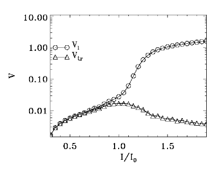
Figure 1.22: Numerical simulations: IV curves for $\Delta=0.1$ ($V_{l}(\circ)$ and $V_{tr}(\triangle)$).

In Fig.1.21 we show current-voltage characteristics, at $T=0.02$ (in units of the Josephson energy, $k_{B}E_{J}$) obtained numerically for an array of $32\times 32$ junctions without ($\Delta=0$) and with disorder($\Delta=0.1$, i.e. $\pm 5$% variation) in the critical currents. The dc current is applied in the diagonal direction ($\phi=45^{o}$), $[1,1]$. We clearly see the appearance of finite transverse voltage, $V_{tr}\neq 0$, with a $5$% of disorder in the critical currents. For low currents longitudinal voltage is equal to transverse voltage and they start to separate when the vortex-antivortex pairs density increases considerably upon increasing current. $V_{tr}$ presents a maximum around $I=I_{0}$ and for larger currents tends to zero. This behaviour is in contrast to the one obtained before without disorder, where $V_{tr}=0$ for all currents. We calculate IV characteristics as a function of the intensity of disorder and we observe, as we show in the inset, that the transverse voltage is almost independent of $\Delta$ in the range considered, $0.1\leq\Delta\leq 0.6$.

In Fig.1.22 we show in a log-log scale our previous results in order to compair them with the experimental results, obtained in an array of $100\times 1000$ proximity–effect Pb/Cu/Pb junctions, at a low temperature $T=1.25K$ and at a low magnetic field (see Fig. 1.20). Qualitatively we get a good agreement between experiments and simulations now in the case of diagonal bias, in opposite to the results obtained without disorder and diagonal bias.

The simulation results presented up to this point were focused in the motion of a single vortex in the periodic pinning of a square JJA. The vortex collective effects, for fields $f>1/L^{2}$, will be discussed below.

Figure 1.23: Parametric curves $V_{y}(\phi)$ vs. $V_{x}(\phi)$ for different dc current applied and temperatures: (a) $|I_{y}|=0.06$ and $T=0.015$, (b) $|I_{y}|=0.06$ and $T=0.03$, (c) $|I_{y}|=0.16$ and $T=0.015$, (d) $|I_{y}|=0.16$ and $T=0.035$.

Breaking of rotational invariance in diluted vortex lattices

In the previous subsection we showed that the “diagonal” [11] direction is unstable against small changes in the angle $\phi$, while the [10] and [01] directions are the preferred directions for single vortex motion [24]. This shows as “horns” in parametric $V_{y}$ vs. $V_{x}$ plots, which are finite segments of points lying in the $x$ or the $y$ axis. This implies the existence of transverse pinning in these directions (thus, it corresponds to orientational pinning). Now we return to the case of diluted vortex lattices ($f=1/25$) and we perform the same analysis as before for the different regimes of the moving VL obtained in Sec. 1.3.4.

In Fig.1.23 we plot the voltages $V_{y}$ and $V_{x}$ when varying the orientational angle $\phi$ for different current amplitudes $I$ and temperatures $T$. In Fig.1.23(a) we have $I=0.06$ and $T=0.015$, corresponding to the regime of a transversely pinned lattice. In this case most of the points are lying either on the axis $V_{x}=0$ or on the axis $V_{y}=0$, indicating strong orientational pinning in the symmetry lattice directions [10] and [01]. When increasing $T$ the orientational pinning decreases and the length of the “horns” in the $x$ and $y$ axis decreases. Fig.1.23(b) shows results for $I=0.06$ and $T=0.03$, which correspond to $T>T_{tr}$ when there is a finite transverse resistance. In this case the horns have disappeared and orientational pinning is lost. However, the breaking of rotational symmetry is still present in the star-shaped curves. Also in the high current regime, Fig.1.23(c), for a low temperature $T=0.015$ ($T<T_{tr}$) we see that there is orientational pinning with the presence of horns, which again disappears for $T>T_{tr}$ as it is shown in Fig.1.23(d) at $T=0.035$. Finally for $T\gg T_{M}$, deep inside in the liquid phase, the stars tend to the circular shape of rotational invariance.

Therefore we have shown that orientational pinning is a useful phenomenon to characterize the different dynamical regimes in JJA, both numerically and experimentally.

1.3.6 Summary and discussion

Figure 1.24: $I-T$ Phase diagram for $f=1/25$. $T_{M}(I)$ line is obtained from $S({\bf G})$ vs. $T$ curves $(\bullet)$. $T_{p}(I)$ line is obtained from IV curves $(\star)$, from $S({\bf G})$ vs. $T$ curves $(\bullet)$ and from $\langle V_{y}\rangle$ vs. $T$ curves $(\triangle)$. $T_{tr}(I)$ curve is obtained from $\langle V_{tr}\rangle$ vs. $T$ curves $(\blacklozenge)$.

With all the information of the previous sections we obtain the current-temperature phase diagram shown in Fig.1.24. For finite currents we have been able to identify three different regimes, a pinned VL for $T<T_{p}(I)$, a transversely pinned VL for $T_{p}(I)<T<T_{tr}(I)$, and a floating VL for $T_{tr}(I)<T<T_{M}(I)$. It is, however, difficult to define if the temperatures $T_{p},T_{tr},T_{M}$ correspond to either phase transitions or to dynamical crossovers. The comparisons we have made of the behavior of voltages (longitudinal and transversal), structure factor and helicity modulus show that something is happening at these temperatures. Also, the comparison for different system sizes of the behavior of $S({\bf G})$ suggest transitions for $T_{p},T_{tr},T_{M}$. The transverse helicity modulus has strong fluctuations for $T_{tr}<T<T_{M}$. These fluctuations are not reduced when increasing the simulation time in a factor of $10$. This could mean that actually the range of temperatures of $T_{tr}<T<T_{M}$ corresponds to a long crossover region towards a liquid state. Also, one may question if the use of the helicity modulus for these far from equilibrium states is correct, since $\Upsilon_{x}$ has been defined from the response of the equilibrium free energy to a twist in the boundary condition. Most likely, the large fluctuations in $T_{tr}<T<T_{M}$ are due to the very unstable and history-dependent steady states we find in this regime. For example the steady states obtained when increasing temperature from $T=0$ at fixed current differ from the steady states obtained when increasing current at fixed temperature in this regime. They differ in the degree of anisotropy and intensity of the Bragg peaks in the structure factor. We think that this reflects the fact that the VL is unpinned in all directions and the orientation of the moving state will depend on the history for this regime.

In any case, we can clearly distinguish different dynamical states which define the regimes shown in the phase diagram of Fig.1.24. From the experimental point of view these transitions (or crossovers) are possible to measure. The depinning temperature $T_{p}$ can be obtained from resistance measurements at finite currents. The transverse current-voltage characteristics and the transverse resistivity can be measured for different longitudinal currents and temperatures, and therefore $T_{tr}$ could be obtained. The helicity modulus can be measured with the two-coil technique [3]. It could be very interesting to see the results of such measurements at finite currents. The structure factor and melting transition can not be measured directly. However, in the presence of an external rf current, the disappearance of Shapiro steps can indicate the melting transition [59], since they are sensitive to the translational order of the vortex lattice [60]. Therefore, we expect that the results obtained here could motivate new experiments for fractional or submatching fields in Josephson junction arrays as well as in other superconductors with periodic pinning.

After our articles (see Ref.[23],[24],[25]) several experimental works appeared. First of all, D. Shalóm and H. Pastoriza designed a new two coil kinetic inductance technique in order to measure transport anisotropy induced by the applied current itself. They found for first time experimental evidence for the anisotropic character of the current driven diluted vortex lattices states in JJA [61]. Later they improved the previous technique, implementing rectangular coils with high aspect radio which are now lithographically fabricated on top of the sample, separated for isolation layers [62].

Regarding numerical works, it is very interesting to mention that recently the disappearance of Shapiro steps was used to indicate the melting transition for another submatching field, $f=1/2$ [63], system which we are going to discuss in next section.

About our results on orientational pinning we would like to do a series of remarks and comments. In the egg-carton potential of a square JJA there are pinning barriers for vortex motion in all the directions. The direction with the lowest pinning barrier is the [10] direction. Therefore the strong orientational pinning we find here is in the direction of the lowest pinning for motion, i.e. the direction of easy flow for vortices. The presence of a strong orientational pinning leads to a large transverse voltage when the systems is driven away from the favorable direction, to the existence of a critical angle and to a transverse critical current. On the other hand, the [11] direction is the direction of the largest barrier for vortex motion in the egg-carton potential. In this case, the behavior is highly unstable against small variations in the angle of the drive, leading to a rapid change from zero transverse voltage to a large transverse voltage within a few degrees. Any misalignment of the current/voltage contacts as well as disorder in the junctions critical currents [27] can lead to a large transverse voltage for arrays with a diagonal bias. This explains the transverse voltage observed experimentally in JJA driven near the diagonal [11] orientation [24].

An analogous effect of orientational pinning has also been seen in experiments on YBCO superconductors with twin boundaries [45]. In this case, due to the correlated nature of the disorder, the direction for easy flow is the direction of the twins. A similar effect of horns in the parametric voltage curves are therefore observed in the direction corresponding to the twins. Also transport measurements when the sample is driven at an angle with respect to the twin show a large transverse voltage.

It is interesting to compare with the angle-dependent transverse voltage calculated for d-wave superconductors [64]. Also in this case, the transverse voltage vanishes only in the [10] and [11] directions. However the $\theta_{t}$ vs. $\phi$ curves are smooth in this case, since $\tan\theta_{t}\propto\sin 4\phi$ [64]. This is because there is no pinning and the transverse voltage is caused only by the intrinsic nature of the d-wave ground state. On the other hand, the breaking of rotational symmetry studied here is induced by the pinning potential, and it results in non-smooth responses like “horned” parametric voltage curves, critical angles, transverse critical currents, etc.

In superconductors with a square array of pinning centers, typically the pins are of circular shape and the size of the pins is much smaller than the distance between pinning sites [16, 18, 19]. In this case, the pinning barriers that vortices find for motion are the same in many directions. Therefore it is possible to have orientational pinning in many of the square lattice symmetry directions. This explains the rich structure of a Devil’s staircase observed recently in the simulations of Reichhardt and Nori, where each plateau corresponds to orientational pinning in each of the several possible directions for orientational pinning. This interesting behavior is not possible in JJA, however, since the egg-carton pinning potential corresponds to the situation of square-shaped pinning centers with the pin size equal to the interpin distance. In this case the only possible directions for orientational pinning are the [10] and [01], as we have seen here.

It is worth noting that many experiments in JJA in the past have been done in samples with a diagonal bias. For example, van Wees et al. [38] have observed the existence of a transverse voltage in their measurements, which was unexplained. From our finding that the [11]-direction is unstable against changes in the angle of the bias, we conclude that any small deviation in the direction of the flow of current, either due to tiny fabrication defects in the busbars or to disorder in the critical currents of the junctions [27], may explain their observation. Also Chen et al.[65] have reported a transverse angle in measurements in JJA driven in the diagonal direction. In their case the effect is antisymmetric against a change in the direction of the magnetic field. Since transverse voltages due to the instability of the [11] direction are even with the direction the magnetic field, their observation can not be explained from our results. This means that they have a Hall effect, possibly due to quantum fluctuations. However, they report that their transverse voltage had also a component which was even with the magnetic field (which was discounted in their computation of the Hall angle). This particular spurious contribution can also be attributed to a small deviation in the direction of the bias or to disorder effects. From this we conclude that in order to study the Hall effect in JJA the most convenient choice would be a current bias in the [10] direction where the effect of transverse voltages at small deviations in the bias or disorder is minimum.

When our work was upon completion, new studies of the effect of the orientation of the bias in driven square JJA have appeared. Fisher, Stroud and Janin [56] have studied some of the effects of the direction of current in a fully frustrated JJA ($f=1/2$) at $T=0$. In their case a transverse critical critical current and the dynamics as a function of $I_{x}$ and $I_{y}$ has been described. Their results are in part complementary to our work with a single vortex ($f=1/L^{2}$). Yoon, Choi and Kim [57] find differences in the IV characteristics of JJA at $f=0$ when comparing the parallel current bias with the diagonal current bias. Their results are in agreement with our results.

It is worth to mention that very recently an experiment in another systems with periodic pinning potentials, in superconductors with a square antidots arrays, evidence of guided vortex motion was observed [66]. They showed that the pinning landscape provided by the square antidot lattice influences the vortex motion, given place to an anisotropic motion, temperature dependent, confirming our results of Sec. 1.3.5.

In summary, in Sec. 1.3.5 of this review we have considered the dynamics of a single vortex in a square JJA and diluted vortex lattices. We were able to characterize in detail the orientational pinning and breaking of rotational symmetry in this case. Furthermore, with the results of the RSJ numerical calculation we were able to reproduce and interpret most of experimental measurements for a quasi-diagonal bias [24]. Regarding the moving vortex lattice different dynamical phases in a JJA, as a function of temperature and current, we also show here that characteristics of the breaking of rotational invariance, orientational pinning and transverse voltages depend on the dynamical phase under consideration as well as on the disorder in the Josephson couplings [27]. Therefore we shown that orientational pinning is a useful tool to characterize the non equilibrium vortex dynamics regimes in JJA, both numerically and experimentally.

1.4 VORTEX DYNAMICS IN FULLY
FRUSTRATED JJA

In this section we show the study of the fully frustrated JJA ($f=1/2$) for system sizes of $L\times L$ junctions, with $L=8,16,24,32,48,64,128$. In the absence of external currents, we find an equilibrium phase transition at $T_{c}=0.45$ which, within a resolution of $\Delta T=0.005$, corresponds to a simultaneous (or very close) breaking of the $U(1)$ and the $Z_{2}$ symmetries. Here we will analyze the possible occurrence of these transitions as a function of temperature when the JJA is driven by currents well above the zero temperature critical current $I>I_{c0}=(\sqrt{2}-1)I_{0}\approx 0.414I_{0}$.

Figure 1.25: For large currents $I>I_{c}(0)$: breaking of the $U(1)$ symmetry. Example showed for $I=0.9$ and system size $64\times 64$. (a) Helicity Modulus $\Upsilon_{x}$ vs temperature $T$ ($\bullet$ increasing $T$, $\Diamond$ decreasing $T$). (b) Transverse voltage for a small transverse current, $I_{tr}=0.1$, vs $T$. (c) Vortex-antivortex pairs density, $n_{va}$ vs. $T$.

1.4.1 $U(1)$ symmetry and transverse superconductivity

In the driven JJA superconducting coherence can only be defined in the direction transverse to the bias current [23, 25, 50]. We calculate the transverse helicity modulus as was shown in Sec. 1.2.3. We find that $\Upsilon_{x}$ is finite at low $T$ and vanishes at a temperature $T_{U(1)}(I)$. In Fig.1.25(a) we show the behavior of $\Upsilon_{x}(T)$ for a current $I=0.9$ in a $64\times 64$ JJA. This transition is reversible: we obtain the same behavior when decreasing $T$ from a random configuration at $T=1$ and when increasing $T$ from an ordered state at $T=0$, see Fig.1.25(a). Transverse superconductivity can be measured when a small current $I_{tr}$ is applied perpendicular to the driving current: we find a vanishingly small transverse voltage $V_{tr}$ below $T_{U(1)}(I)$, as we found before in [23, 25] for $f=1/25$. We obtain the voltage in the $\mu$-direction as the time average $V_{\mu}=\langle d\alpha_{\mu}(t)/dt\rangle$ (normalized by $R_{N}I_{0}$); longitudinal voltage is $V=V_{y}$ and transverse voltage is $V_{tr}=V_{x}$. In Fig.1.25(b) we see that the transverse resistance $V_{tr}/I_{tr}$ is negligibly small for $T<T_{U(1)}$ and starts to rise near the transition. The equilibrium $U(1)$ transition (at $f=0$, $I=0$, Kosterlitz-Thouless) is characterized by the unbinding of vortex-antivortex pairs above $T_{c}$. We calculate the density $n_{va}$ of vortex-antivortex excitations above checkerboard vortex configuration as $2n_{va}=\langle|b({\bf\tilde{n}})|\rangle-f$, where the vorticity at the plaquette ${\bf\tilde{n}}$ (associated to the site ${\bf n}$) is $b({\bf\tilde{n}})=-\Delta_{\mu}\times{\rm nint}[\theta_{\mu}({\bf n})/2\pi]$. We see in Fig.1.25(c) that $n_{va}$ rises near $T_{U(1)}$. Moreover, the transverse resistivity above $T_{U(1)}$ is $V_{tr}/I_{tr}\propto n_{va}$.

In Fig.1.26 shows $\Upsilon_{x}$ for sizes $L=32,48,64,128$, we see that a transition temperature can be defined independently of lattice size.

Figure 1.26: Helicity Modulus $\Upsilon_{x}$ vs temperature $T$ for $I=0.9$ and system size $64\times 64$, increasing $T$. Size effect for $L=32,48,64,128$.

1.4.2 $Z_{2}$ symmetry

Figure 1.27: For a large currents, $I>I_{c}(0)$: breaking of the $Z_{2}$ symmetry. Example shown for a dc current $I=0.9$ and system size $128\times 128$. Results for increasing $T$ ($\bullet$) and decresing $T$ ($\Diamond$). (a) Chiral order parameter $\chi$ vs $T$ and one-dimensional order parameter $\chi_{x}$ vs. $T$. Inset: size effect for $\chi$ for $L=8,16,32,48,64,128$. (b) Longitudinal voltage $V$ vs. $T$. (c) Domain wall lengths ${\cal L}_{x}$ and ${\cal L}_{y}$ vs. $T$. Inset: domain anisotropy ${\cal L}_{x}/{\cal L}_{y}$ vs. $T$.

Since the ground state is a checkerboard pattern of vortices, we define the “staggered magnetization” as $m_{s}({\bf\tilde{n}},t)=(-1)^{n_{x}+n_{y}}[2b(n_{x},n_{y},t)-1]$ and $m_{s}(t)=(1/L^{2})\sum_{\bf\tilde{n}}m_{s}({\bf\tilde{n}},t)$. At $T=0$, $I=0$ there are two degenerate configurations with $m_{s}=\pm 1$. Above the $T=0$ critical current $I_{c0}$ the checkerboard state moves as a rigid structure and $m_{s}(t)$ changes sign periodically with time. Therefore we define the chiral order parameter as $\chi=\langle m_{s}^{2}(t)\rangle$. We start the simulation at $T=0$ with an ordered checkerboard state driven by a current $I>I_{c0}$ and then we increase slowly the temperature. We obtain that the chirality parameter vanishes at a temperature $T_{Z_{2}}$, which is smaller than $T_{U(1)}$, as can be seen in Fig.1.27(a) for $I=0.9$. This transition is confirmed by the size analysis shown in the inset of Fig.1.27(a): for $T<T_{Z_{2}}$ the chirality $\chi$ is independent of size, while for $T>T_{Z_{2}}$ we see that $\chi\sim 1/L^{2}$. As it is shown in Fig.1.27(b), the longitudinal voltage $V$ has a sharp increase at $T_{Z_{2}}$, which could be easily detected experimentally. The excitations that characterize the $Z_{2}$ transition are domain walls that separate domains with different signs of $m_{s}$. The length of domain walls in the direction $\mu$ is given by ${\cal L}_{\mu}=(2/L^{2})\sum_{\bf\tilde{n}}\langle b({\bf\tilde{n}})b({\bf\tilde{n}}+{\bf\nu})\rangle$, with $\nu\perp\mu$. We find that for $I>0$ and $T>0$ the domains are anisotropic, with the domain walls being longer in the direction perpendicular to the current (${\cal L}_{x}>{\cal L}_{y}$) and the domain anisotropy ${\cal L}_{x}/{\cal L}_{y}$ increasing with $I$. In Fig.1.27(c) we show the dependence of ${\cal L}_{\mu}$ with temperature for $I=0.9$. At $T=0$ there are no domain walls, since the initial condition is the checkerboard state, and the domain wall length grows with $T$, showing a sharp increase at $T_{Z_{2}}$. The domain anisotropy ${\cal L}_{x}/{\cal L}_{y}$ is shown in the inset of Fig.1.27(c): it has a clear jump at the transition in $T_{Z_{2}}$ while for $T\gg T_{Z_{2}}$ the domains tend to be less anisotropic. When decreasing temperature from a random configuration at $T=1$, an important number of domain walls along the $x$ direction remain frozen below $T_{Z_{2}}$: ${\cal L}_{x}$ tends to a finite value when $T\rightarrow 0$ and the domain anisotropy tends to diverge when cooling down. This leads to a strong hysteresis in the voltage $V$ at $T_{Z_{2}}$ (see Fig.1.27(b)) since the extra domain walls increase dissipation [39, 67]. This low $T$ state with frozen-in domain walls is ordered along the $x$-direction (i.e. perpendicular to $I$) but is disordered along the $y$ direction which gives $\chi\approx 0$. We define the $Z_{2}$ order parameter in the $x$ direction as $\chi_{x}=\langle(1/L)\sum_{n_{y}}[(1/L)\sum_{n_{x}}m_{s}(n_{x},n_{y},t)]^{2}\rangle$ and $\chi_{y}$ is defined analogously. We see in Fig.1.27(a) that, when cooling down from high $T$, $\chi_{x}$ vanishes as $\chi_{x}\sim 1/L$ for $T>T_{Z_{2}}$ (it has stronger size effects than $\chi$) and becomes finite for $T<T_{Z_{2}}$, while $\chi_{y}\approx 0$ for any $T$. Therefore, depending on the history, there are two kinds of high current steady states with broken $Z_{2}$ symmetry at low $T$. One state has mostly the checkerboard structure ($\chi\not=0$) with few very anisotropic domains. It can be obtained experimentally by cooling down at zero drive and then increasing $I$. The other steady state is ordered in the direction perpendicular to $I$ ($\chi_{x}\not=0$, $\chi_{y}=0$) with several domain walls along the $x$ direction. These domain walls move in the direction parallel to $I$ (via the motion of vortices perpendicular to $I$) giving an additional dissipation. This state can be obtained experimentally by cooling down with a fixed $I$.

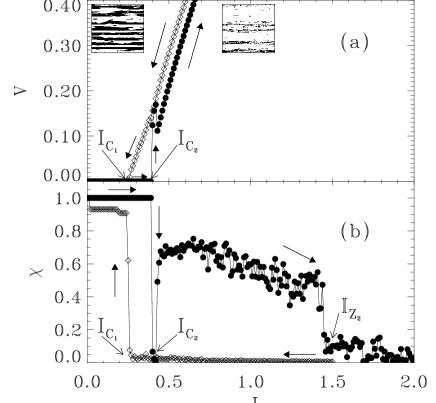
Figure 1.28: Current-voltage hysteresis for $T=0.02$ shown for (a) voltage vs. $I$ and (b) chiral order parameter vs. $I$. Increasing current from the checkerboard state ($\bullet$) and decreasing current from a random state at large $I>I_{Z_{2}}$ ($\Diamond$). Insets: snapshots of the staggered magnetization $m_{s}({\bf n},t)$: almost perfect ordered state obtained increasing current (right), and ordered state with ${\cal L}_{x}$-domain walls obtained decreasing current (left).

The two steady states have also different critical currents as can be observed in the low $T$ current-voltage (IV) characteristics. In Fig.1.28(a) we show the IV curve for $T=0.02$ and in Fig 1.28(b) the corresponding $\chi$ vs. $I$ curve. When increasing $I$ from the $I=0$ equilibrium state, we find a critical current $I_{c2}(T)$, which in the limit of $T=0$ tends to $I_{c0}=\sqrt{2}-1$ as found analitically and in simulations with PBC [36, 68, 69]. Near $I_{c2}$ the order parameter $\chi$ has a minimum and rapidly increases with $I$. The driven state is an ordered state similar to the one shown in Fig.1.27(a) (see right inset). At a higher current $I_{Z_{2}}$ there is a sharp drop of $\chi$ which corresponds to the crossing of the $T_{Z_{2}}(I)$ line (see Fig.1.29) and the $Z_{2}$ order is lost. If we now decrease the current either from the disordered state at $I>I_{Z_{2}}$ or from a random initial configuration or from a configuration cooled down at a fixed $I>I_{c2}$, we obtain the steady state with domain walls along the $x$ direction and $\chi\approx 0,\chi_{x}\not=0$ (see left inset). This state has a higher voltage and pins at a lower critical current $I_{c1}(T)$, which has the $T=0$ limit $I_{c1}(T\rightarrow 0)=0.35$. It has been shown [69] that open boundary conditions can nucleate domain walls leading to the critical current $I_{c1}(0)=0.35$ usually found in open boundary $T=0$ simulations [39, 46, 47, 67]. Also a moving state with parallel domain walls (as in the insets of Fig.1.28(a)) has been found by Grønbech-Jensen et al. [70] in $f=1/2$ JJA with open boundaries and Marino and Halsey [71] have shown that the high current states of frustrated JJA can have moving domain walls. We have studied the effect of open boundaries in the direction of $I$, in the direction perpendicular to $I$ and in both directions. They differ mainly in the $T=0$ critical current and IV curve, for finite $T$ there are small differences in the detailed shape of the hysteresis in critical current. In all the cases the two high current steady states are observed at finite $T$ with the same history dependence. Also, we find that the density of frozen ${\cal L}_{x}$ domain walls depends on cooling rate and decreases with system size.

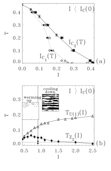
Figure 1.29: Current-temperature phase diagrams: (a) for low currents, $I<I_{c}(0)$ and (b) for high currents, $I>I_{c}(0)$. $I_{c1}(T)$ ($\Diamond$) and $I_{c2}(T)$ ($\bullet$) lines are obtained from hysteresis in IV curves as well as from hysteresis in $\Upsilon_{x}(T)$ and $\chi(T)$ curves. $T_{U(1)}(I)$ line obtained from $\Upsilon_{x}(T)$ and $V_{tr}(T)$ ($\triangle$). $T_{Z_{2}}(I)$ line obtained from $\chi(T)$, $V(T)$ and ${\cal L}_{x}/{\cal L}_{y}(T)$ ($\bullet$). The dashed line corresponds to the IV curve of previous Fig. ($T=0.02$). Insets: Two different steady states (staggered magnetization snapshots) found below $T_{Z_{2}}(I)$ line, at $T=0.02$ and $I=0.9$: (i) warming up, almost a perfect checkerboard pattern, or (ii) cooling down, ordered state with ${\cal L}_{x}$-domain walls.

1.4.3 Summary

In summary, we have obtained the current-temperature phase diagram of the driven fully frustated XY model, which is shown in Fig.1.29(a) for low currents and in Fig.1.29(b) for high currents. At high currents the breaking of the $U(1)$ and the $Z_{2}$ symmetries occurs at well separated temperatures, with $T_{Z_{2}}<T_{U(1)}$. The low temperature regime $T<T_{Z_{2}}(I)$ has bistability with two possible steady states (see insets in Fig.1.29) and history dependent IV curves. The different transitions could be observed experimentally with measurements of the transverse and longitudinal voltage.

1.5 CONCLUSIONS

We presented a detailed review of our previous numerical studies on non equilibrium vortex dynamics in JJA driven by a dc current. Dynamical phase diagrams for different magnetic field corresponding to $f=1/25$ and $f=1/2$, current directions (orientational pinning) and varying temperature were obtained and shown in Fig.1.24 and Fig.1.29.

In conclusion for diluted vortex lattices we find that for low currents the depinning transition of the VL and the later melting of the moving VL become separated with $T_{M}(I)>T_{p}(I)$. For large currents we find that the moving VL has a finite transverse critical current and therefore transverse superconducting coherence. In this case it is possible to define a transverse depinning transition at a temperature $T_{tr}$, and a later melting transition of the moving VL at $T_{M}(I)$. This transverse depinning transition could be easily studied in controlled experiments in Josephson junction arrays, both with transport measurements and with inductive coil measurements of the transverse helicity modulus. This proposed experiment were later performed [61] and the anisotropy of moving vortex phases was confirmed.

Regarding fully frustrated JJA we obtain the current-temperature phase diagram. At high currents (Fig.1.29(b)) we find $T_{Z_{2}}<T_{U(1)}$, which is in contrast with the equilibrium result of $T_{Z_{2}}\simeq T_{U(1)}$ [1,5]. Interestingly, the frustrated XY model with modulated anisotropic couplings also has $T_{Z_{2}}<T_{U(1)}$ [37], meaning that the anisotropy induced by the current may provide a similar effect. It is clear that the $f=1/2$ case has a strong pinning effect (with $I_{c0}=0.414$) when compared to the dilute case of $f=1/25$ (with $I_{c0}=0.11$) [23, 25]. In fact, the transverse depinning temperature $T_{U(1)}$ is one order of magnitude higher for $f=1/2$ with respects to $f=1/25$ [23]. The driving current weakens the effect of pinning and thus $T_{U(1)}$ increases with $I$. A similar effect gives a $T_{Z_{2}}$ growing with $I$ just above $I_{c0}$. However for larger currents (near the Josephson current $I_{0}$) $T_{Z_{2}}(I)$ starts to decrease with $I$, with the limit $T_{Z_{2}}(I\rightarrow\infty)\rightarrow 0$. This is because a driving current increases the density of domain walls (an effect already mentioned in [39]) destroying the Ising order for $I\gg I_{c0}$. Moreover, we find that the ordered region in $T<T_{Z_{2}}(I)$ has bistability with two possible steady states and history dependent IV curves. The different transitions here characterized could be obtained experimentally by measurements of transverse and longitudinal voltage. With our numerical results on highly driven fully frustrated JJA we expect to motivate an experimental confirmation of the clear separation of the transition temperatures, $T_{Z_{2}}<T_{U(1)}$.

Appendix A: Periodic boundary conditions

Phases

We want to obtain the periodic boundary condition (PBC) for superconducting phases $\theta(n_{x},n_{y})$. In general we can write the PBC as:

$$\theta({\bf n}+{\bf L_{x}}) = \theta({\bf n})+u_{x}({\bf n})$$

$$\theta({\bf n}+{\bf L_{y}}) = \theta({\bf n})+u_{y}({\bf n})\;,$$ (1.28)

where ${\bf L_{x}}=(L_{x},0)$ and ${\bf L_{y}}=(0,L_{y})$. Taking into account that all variables should be independent of the order of subsequent global translations and that the phases are defined except for an addition of $2\pi l$, we are lead to the consistency condition

$$u_{x}({\bf n})+u_{y}({\bf n}+{\bf L_{x}})=u_{x}({\bf n}+{\bf L_{y}})+u_{y}({\bf n})+2\pi l\;,$$ (1.29)

Therefore, in order to specify the periodic boundary conditions we have to give the functions $u_{x},u_{y}$, which will depend on the gauge for the vector potential ${\bf A}$.

The periodic boundary condition for the phases can be deduced by requiring that all physical quantities are invariant after a translation in the lattice size. The supercurrents $S_{\mu}({\bf n})=\sin[\Delta_{\mu}\theta({\bf n})-A_{\mu}({\bf n})]$ should satisfy:

$$S_{\mu}({\bf n}+{\bf L_{x}}) = S_{\mu}({\bf n})$$

$$S_{\mu}({\bf n}+{\bf L_{y}}) = S_{\mu}({\bf n})\;.$$ (1.30)

This implies that the gauge invariant phase difference $\theta_{\mu}({\bf n})=\Delta_{\mu}\theta({\bf n})-A_{\mu}({\bf n})$ should satisfy

$$\theta_{\mu}({\bf n}+{\bf L_{x}}) = \theta_{\mu}({\bf n})+2\pi l$$

$$\theta_{\mu}({\bf n}+{\bf L_{y}}) = \theta_{\mu}({\bf n})+2\pi l^{\prime}\;,$$ (1.31)

with $l,l^{\prime}$ any integer. This condition leads to

$$\Delta_{\mu}u_{x}({\bf n}) = 2\pi l+A_{\mu}({\bf n}+{\bf L_{x}})-A_{\mu}({\bf n})$$

$$\Delta_{\mu}u_{y}({\bf n}) = 2\pi l^{\prime}+A_{\mu}({\bf n}+{\bf L_{y}})-A_{\mu}({\bf n})\;.$$ (1.32)

We can choose the solution with $l=l^{\prime}=0$. In the Landau gauge, $A_{x}$ is a linear function of $n_{y}$ and $A_{y}$ is a linear function of $n_{x}$. Taking the origin such that $A_{\mu}({\bf n}=0)=0$, we obtain for the Landau gauge:

$$u_{x}({\bf n}) = u_{x}(0)+A_{y}({\bf L_{x}})n_{y}$$

$$u_{y}({\bf n}) = u_{y}(0)+A_{x}({\bf L_{y}})n_{x}\;.$$ (1.33)

The consistency condition (1.29) requires

$$A_{y}({\bf L_{x}})L_{y}-A_{x}({\bf L_{y}})L_{x}=2\pi l\;.$$ (1.34)

The term in the left side is equal to the total flux $2\pi fL_{x}L_{y}$, therefore (1.34) is equivalent to flux quantization, giving $fL_{x}L_{y}=N_{v}$, with $N_{v}=l$ the number of vortices.

If we take $u_{x}(0)=u_{y}(0)=0$, we obtain for the PBC

$$\theta(n_{x}+L_{x},n_{y}) = \theta(n_{x},n_{y})+A_{y}({\bf L_{x}})n_{y}$$

$$\theta(n_{x},n_{y}+L_{y}) = \theta(n_{x},n_{y})+A_{x}({\bf L_{y}})n_{x}.$$ (1.35)

A particular choice can be the gauge with $A_{x}({\bf n})=-2\pi fn_{y}$, $A_{y}({\bf n})=0$, which leads to Eq. 1.8.

External currents and electric fields

In the presence of external currents or voltages the periodic boundary conditions have to be reconsidered. In this case it is possible to have $\oint{\bf E}\cdot{\bf dl}\not=0$ in a path that encloses all the sample either in the $x$ or the $y$ direction. Therefore, in a closed path we have to consider the Faraday’s law

$$\oint{\bf E}\cdot{\bf dl}=-\frac{1}{c}\frac{d\Phi}{dt}.$$

The two-dimensional sample with PBC can be thought as the surface of a torus in three-dimensions. The closed paths we are considering are the two pathes that encircle the torus. The electric field is not a gradient of a potential, it is now given by ${\bf E}=-{\bf\nabla}V-\frac{1}{c}\frac{\partial{\bf A}}{\partial t}$. One possible solution is to consider a vector potential

$${\bf A}({\bf r},t)={\bf A_{0}}({\bf r})-{\bf\vec{\alpha}}(t),$$

for which

$${\bf H}_{\rm ext} = {\bf\nabla}\times{\bf A_{0}}$$

$${\bf E}_{\rm total} = \frac{1}{c}\frac{d{\bf\vec{\alpha}}}{dt}$$

In our case, we take the adimensional vector potential as:

$$A_{\mu}({\bf n},t)=A_{\mu}^{0}({\bf n})-\alpha_{\mu}(t),$$ (1.36)

with $A_{\mu}^{0}({\bf n})$ in the Landau gauge ($A_{x}^{0}({\bf n})=-2\pi fn_{y}$, $A_{y}^{0}({\bf n})=0$). Therefore the gauge invariant phase is:

$$\theta_{\mu}({\bf n},t)=\Delta_{\mu}\theta({\bf n},t)-A^{0}_{\mu}({\bf n})+\alpha_{\mu}(t).$$

Then $\alpha_{\mu}$ acts as a global time-dependent phase in the $\mu$ direction.

In the normalized units used in this paper, the electric field in the link defined by the junction ${\bf n},\mu$ is

$$E_{\mu}({\bf n})=-\Delta_{\mu}V({\bf n})-\frac{dA_{\mu}({\bf n})}{dt},$$

where the electrostatic potential is $V({\bf n})=-\frac{d\theta({\bf n})}{dt}$. Therefore we have

$$E_{\mu}({\bf n})=\Delta_{\mu}\frac{d\theta({\bf n})}{dt}+\frac{d\alpha_{\mu}}{dt}.$$

The average electric field in the $\mu$ direction is:

$$E^{\rm av}_{\mu}=\frac{1}{L_{x}L_{y}}\sum_{\bf n}E_{\mu}({\bf n})=\frac{d\alpha_{\mu}}{dt},$$

where we have used the fact that $\sum_{\bf n}\Delta_{\mu}\frac{d\theta({\bf n})}{dt}=0$ (which is the discrete equivalent of $\oint{\bf\nabla}V\cdot{\bf dl}=0$). The current in the link ${\bf n},\mu$ is, in normalized units,:

$$I_{\mu}({\bf n})=E_{\mu}({\bf n})+\tilde{S}_{\mu}({\bf n}),$$

with $\tilde{S}_{\mu}({\bf n})=S_{\mu}({\bf n})+\eta_{\mu}({\bf n},t)$. Therefore the average current in the $\mu$ direction is

$$I^{\rm av}_{\mu} = \frac{1}{L_{x}L_{y}}\sum_{\bf n}I_{\mu}({\bf n})$$

$$= E^{\rm av}_{\mu}+S^{\rm av}_{\mu}+\eta^{\rm av}_{\mu}=\frac{d\alpha_{\mu}}{dt}+\frac{1}{L_{x}L_{y}}\sum_{\bf n}\tilde{S}_{\mu}({\bf n})$$

There are two cases to consider: (i) external current source: the external current is given and the total voltage fluctuates and (ii) external voltage source: the external voltage is given and the total current fluctuates.

(i) External current source: the average current in $\mu$ direction is fixed by the external current: $I^{\rm av}_{\mu}=I_{\mu}^{\rm ext}$. The average electric field is a fluctuating quantity given by:

$$E^{\rm av}_{\mu}(t)=\frac{d\alpha_{\mu}}{dt}=I^{\rm ext}_{\mu}-\frac{1}{L_{x}L_{y}}\sum_{\bf n}\tilde{S}_{\mu}({\bf n}).$$ (1.37)

In this case, the $\alpha_{\mu}(t)$ is a dynamical variable, and its time evolution is given by Eq. 1.37.

(ii) External voltage source: the average electric field in the $\mu$ direction is fixed by the external electric field: $E^{\rm av}_{\mu}=E_{\mu}^{\rm ext}$. Therefore, now the $\alpha_{\mu}$ is given by the external source:

$$\alpha_{\mu}(t)=\int E_{\mu}^{\rm ext}dt,$$

and $\alpha_{\mu}(t)=E_{\mu}^{\rm ext}t$, if $E_{\mu}^{\rm ext}$ is time-independent. The average current is now a fluctuating quantity given by:

$$I^{\rm av}_{\mu}=E_{\mu}^{\rm ext}+\frac{1}{L_{x}L_{y}}\sum_{\bf n}\tilde{S}_{\mu}({\bf n}).$$

Let us see how the PBC are affected by a change of gauge. The gauge transformations are the following:

$$\theta({\bf n})\rightarrow\theta^{\prime}({\bf n}) = \theta({\bf n})+\phi({\bf n})$$

$$A_{\mu}({\bf n})\rightarrow A^{\prime}_{\mu}({\bf n}) = A_{\mu}({\bf n})+\Delta_{\mu}\phi({\bf n})$$

$$V({\bf n})\rightarrow V^{\prime}({\bf n}) = V({\bf n})-\frac{d\phi({\bf n})}{dt}$$

An interesting choice is:

$$\phi({\bf n})=\vec{\alpha}\cdot{\bf n}=\sum_{\mu}\alpha_{\mu}n_{\mu}$$

In this gauge we have $\theta_{\mu}({\bf n})=\Delta_{\mu}\theta({\bf n})-A^{0}_{\mu}({\bf n})$ and the PBC for the phases is:

$$\theta({\bf n}+{\bf L_{x}}) = \theta({\bf n})+A_{y}({\bf L_{x}})n_{y}+\alpha_{x}L_{x}$$

$$\theta({\bf n}+{\bf L_{y}}) = \theta({\bf n})+A_{x}({\bf L_{y}})n_{x}+\alpha_{y}L_{y},$$ (1.38)

and for the voltages:

$$V({\bf n}+{\bf L_{\mu}})=V({\bf n})-\frac{d\alpha_{\mu}}{dt}L_{\mu}=V({\bf n})-E^{\rm av}_{\mu}L_{\mu}$$ (1.39)

The equations of motion in this gauge are:

$$\frac{d\theta({\bf n})}{dt} = \sum_{\mu}\frac{d\alpha_{\mu}}{dt}n_{\mu}-\sum_{\bf n^{\prime}}G_{{\bf n},{\bf n^{\prime}}}\Delta_{\mu}\cdot\tilde{S}_{\mu}({\bf n^{\prime}})$$

$$\frac{d\alpha_{\mu}}{dt} = I^{\rm ext}_{\mu}-\frac{1}{L_{x}L_{y}}\sum_{\bf n}\tilde{S}_{\mu}({\bf n})$$ (1.40)

The periodic boundary conditions with a fixed external current using Eq. 1.37 was used previously in Ref. [72] for $f=0$ (it was called a “fluctuating twist boundary condition”) and in Ref. [35] for $f\not=0$. Also, the periodic boundary conditions in the gauge of Eqs. 1.38 and 1.39 were used in Ref. [64] for a time dependent $d$-wave Ginzburg-Landau model.

Helicity modulus

The helicitity modulus $\Upsilon_{\mu}$ expresses the “rigidity” of the system with respect to an applied “twist” in the periodic boundary conditions. The twist $k_{\mu}$ is defined as a phase change of $L_{\mu}k_{\mu}$ between the two opposite boundaries which are connected through the PBC in the $\mu$ direction

$$\theta({\bf n}+{\bf L_{\mu}})=\theta({\bf n})+L_{\mu}k_{\mu}.$$

The helicity modulus is obtained from the free energy $F(T,k_{\mu})$ as:

$$\Upsilon_{\mu}=\left.\frac{1}{L^{2}}\frac{\partial^{2}F(T,k_{\mu})}{\partial k_{\mu}^{2}}\right|_{k_{\mu}=0}$$ (1.41)

It is clear from Eq. 1.38 that $k_{\mu}=\alpha_{\mu}$. Then, in order to evaluate the helicity modulus, $\alpha_{\mu}$ must be set to zero. This means that the helicity modulus can not be calculated in the direction in which there is an applied current, since it gives a fluctuating twist $k_{\mu}(t)$.

Appendix B: Algorithm

The core of the numerical calculation is to invert the Eq. 1.10. This means to solve a discrete Poisson equation of the form,

$$\Delta_{\mu}^{2}f({\bf n})=d({\bf n})$$ (1.42)

with the periodic boundary conditions

$$f({\bf n}+{\bf L_{x}}) = f({\bf n})$$

$$f({\bf n}+{\bf L_{y}}) = f({\bf n})\;.$$ (1.43)

The linear system of $L_{x}L_{y}$ equations of (1.42) is singular. Physically, the reason is that in Eq.(1.10), $f({\bf n})=d\theta({\bf n})/dt$ corresponds to a voltage, which is defined except for a constant. We choose the voltage reference such that it has zero mean:

$$\sum_{\bf n}f({\bf n})=0\;,$$ (1.44)

other choices are also possible (like, for example, fixing $f({\bf n_{0}})=0$ at a given site ${\bf n}_{0}$).

The method we use to invert the Eq. (1.42) is based on the Fourier Accelerated and Cyclic Reduction (FACR) algorithm [73]. In this case, we take first the discrete Fourier transform in the $x$ direction:

$$\tilde{d}(k_{x},n_{y})=\sum_{n_{x}}d(n_{x},n_{y})e^{i\frac{2\pi k_{x}n_{x}}{L_{x}}}\;,$$ (1.45)

which with a fast Fourier algorithm takes a computation time of order $L_{x}\log L_{x}$. This leads to the following equation:

$$\epsilon_{k_{x}}\tilde{f}(k_{x},n_{y})-\tilde{f}(k_{x},n_{y}-1)-\tilde{f}(k_{x},n_{y}+1)=\tilde{d}(k_{x},n_{y})\;,$$ (1.46)

with $\epsilon_{k_{x}}=4-2\cos\frac{2\pi k_{x}}{L_{x}}$ and with boundary condition $\tilde{f}(k_{x},L_{y}+1)=\tilde{f}(k_{x},1)$. This is a cyclic tridiagonal equation which can be solved with a simple LU decomposition algorithm in a computation time of order $L_{y}$ [73]. In this way the $\tilde{f}(k_{x},n_{y})$ is obtained from (1.46). Finally we take the inverse Fourier transform to obtain

$$f(n_{x},n_{y})=\frac{1}{L_{x}}\sum_{k_{x}}\tilde{f}(k_{x},n_{y})e^{-i\frac{2\pi k_{x}n_{x}}{L_{x}}}\;.$$ (1.47)

This algorithm takes a computation time which is of order $L_{x}L_{y}(\log L_{x}+A)$ with the constant $A\sim 1$. This is faster than the two dimensional Fourier transform method used by Eikmans and van Himbergen [48], which takes a computation time of order $L_{x}L_{y}(\log L_{x}+\log L_{y})$.

Acknowledgments

We acknowledge fruitful discussions with H. Pastoriza, D. Shalóm, J.V. José, E. Granato and useful comments that helped to get this final version, from P. Martinoli. This work was supported by CONICET, ANPCYT PICT99-03-06343, CNEA P5-PID-93-7, Fundacion Antorchas P14116-147 and Swiss National Science Foundation.

Bibliography

- [1] P. Martinoli, O. Daldini, C. Leemann, and E. Stocker, Solid State Comm. 17, 205 (1975); P. Martinoli, O. Daldini, C. Leemann, and B. Van den Brandt, Phys. Rev. Lett. 36, 382 (1976).
- [2] B. Pannetier, J. Chaussy, R. Rammal, and J. C. Villegier, Phys. Rev. Lett. 53, 1845 (1984); H. D. Hallen, R. Seshadri, A. M. Chang, R. E. Miller, L. N. Pfeiffer, K. W. West, C. A. Murray, and H. F. Hess, Phys. Rev. Lett. 71, 3007 (1993); K. Runge and B. Pannetier, Europhys. Lett. 24, 737 (1993).
- [3] For recent reviews in Josephson arrays see R. S. Newrock, C. J. Lobb, U. Geigenmuller and M. Octavio, Solid State Physics 54, 263 (2000); Lectures on superconducting networks and mesoscopic systems, Ed. C. Giovanella and C. J. Lambert (American Institute of Physics, AIP Conf. Proc. 427, New York, 1998) See also J. C. Ciria and C. Giovanella, J. Phys. Condes. Matter 10, 1453 (1998); Macroscopic Quantum Phenomena and Coherence in Superconducting Networks, Ed. C. Giovanella and M. Tinkham (World Scientific, Singapore, 1995) and Proceedings of the ICTP Workshop on Josephson-junction arrays, Physica B 222, 253 (1996).
- [4] C. J. Lobb, D. W. Abraham. and M. Tinkham, Phys. Rev. B 27, 150 (1983).
- [5] See for example M. S. Rzchowski, S. P. Benz, M. Tinkham, and C. J. Lobb, Phys. Rev. B 42, 2041 (1990).
- [6] J. I. Martín, M. Vélez, J. Nogués, and Ivan K. Schuller, Phys. Rev. Lett. 79, 1929 (1997); D. J. Morgan and J. B. Ketterson, Phys. Rev. Lett. 80, 3614 (1998); Y. Jaccard, J. I. Martín, M.C. Cyrille, M. Vélez, J. L. Vicent, and Ivan K. Schuller, Phys. Rev. B 58, 8232 (1998); M. J. Van Bael, K. Temst, V. V. Moshchalkov, and Y. Bruynseraede, Phys. Rev. B 59, 14674 (1999); J. I. Martín, M. Vélez, A. Hoffmann, Ivan K. Schuller, and J. L. Vicent, Phys. Rev. Lett. 83, 1022 (1999); T. Puig, E. Rosseel, L. Van Look, M. J. Van Bael, V. V. Moshchalkov, and Y. Bruynseraede, Phys. Rev. B 58, 5744 (1998).
- [7] M. Baert, V. V. Metlushko, R. Jonckheere, V. V. Moshchalkov, and Y. Bruynseraede, Phys. Rev. Lett 74, 3269 (1995); K. Harada, O. Kamimura, H. Kasai, T. Matsuda, A. Tonomura and V. V. Moshchalkov, Science 274, 1167 (1996); J. Y. Lin, M. Gurvitch, S. K. Tolpygo, A. Bourdillon, S. Y. Hou, and J. M. Phillips, Phys. Rev. B 54, R12717 (1996); A. Bezryadin, Yu. B. Ovchinnikov, and B. Pannetier, Phys. Rev. B 53, 8553 (1996); E. Rosseel, M. Van Bael, M. Baert, R. Jonckheere, V. V. Moshchalkov, and Y. Bruynseraede, Phys. Rev. B 53, R2983, (1996); A. Castellanos, R. Wondenweber, G. Ockenfuss, A. v.d. Hart, and K. Keck, Appl. Phys. Lett. 71, 962 (1997); V. V. Moshchalkov, M. Baert, V. V. Metlushko, E. Rosseel, M. J. van Bael, K. Temst, Y. Bruynseraede, and R. Jonckheere, Phys. Rev. B 57, 3615 (1998); V. Metlushko, U. Welp, G. W. Crabtree, Zhao Zhang, S. R. J. Brueck, B. Watkins, L. E. DeLong, B. Ilic, K. Chung, and P. J. Hesketh, Phys. Rev. B 59, 603 (1999); V. Metlushko, U. Welp, G. W. Crabtree, R. Osgood, S. D. Bader, L. E. DeLong, Zhao Zhang, S. R. J. Brueck, B. Ilic, K. Chung, and P. J. Hesketh, Phys. Rev. B 60, 12585 (1999); L. V. Look, L. Van Look, E. Rosseel, M. J. Van Bael, K. Temst, V. V. Moshchalkov, and Y. Bruynseraede, Phys. Rev. B 60, R6998 (1999).
- [8] S. B. Field, S. S. James, J. Barentine, V. Metlushko, G. Crabtree, H. Shtrikman, B. Ilic, and S. R. J. Brueck, Phys. Rev. Lett. 88, 067003 (2002).
- [9] Y. Fasano, J. A. Herbsommer, F. de la Cruz, F. Pardo, P. L. Gammel, E. Bucher and D. J. Bishop, Phys. Rev. B 60, R15047 (1999).
- [10] P. Martinoli, Phys. Rev. B 17, 1175 (1978).
- [11] V. L. Pokrovskii and A. L. Talanov, Sov. Phys. JETTP 51, 134 (1980).
- [12] P. Martinoli, M. Nsabimana, G. A. Racine and H. Beck, Hel. Phys. Acta 55, 655 (1982).
- [13] D. R. Nelson in Phase Transitions and Critical Phenomena, edited by C. Domb and J. L. Lebowitz (Academic, New York, 1983), Vol. 7.
- [14] M. Franz and S. Teitel, Phys. Rev. Lett. 73, 480 (1994) and Phys. Rev. B 51, 6551 (1995).
- [15] S. Hattel and J. M. Wheatley, Phys. Rev. B 51, 11951 (1995).
- [16] C. Reichhardt, C. J. Olson and F. Nori, Phys. Rev. B 54, 16108 (1996); Phys. Rev. B 57, 7937 (1998).
- [17] W. A. M. Morgado and G. Carneiro, Physica C 238, 195 (1998).
- [18] C. Reichhardt, C. J. Olson and F. Nori, Phys. Rev. Lett. 78, 2648 (1997); Phys. Rev. B 58, 6534 (1998).
- [19] C. Reichhardt and F. Nori, Phys. Rev. Lett. 82, 414 (1999).
- [20] G. Carneiro, J. Low Temp. Phys. 177, 1323 (1999).
- [21] C. Reichhardt, G. Zimanyi, Phys. Rev. B 61, 14354 (2000).
- [22] G. Carneiro, Phys. Rev. B 62, R14661 (2000).
- [23] V. I. Marconi and D. Domínguez, Phys. Rev. Lett, 82, 4922 (1999).
- [24] V. I. Marconi, S. Candia, P. Balenzuela, H. Pastoriza, D. Domínguez and P. Martinoli, Phys. Rev. B, 62, 4096 (2000).
- [25] V. I. Marconi and Domínguez, Phys. Rev. B, 63, 174509 (2001).
- [26] V. I. Marconi and D. Domínguez, Phys. Rev. Lett, 87, 017004, (2001).
- [27] V. I. Marconi, H. Pastoriza and D. Domínguez, J. L. Tem. Phys., Vol 135, 135, (2004).
- [28] L. L. Sohn, M.S. Rzchowski, J.U. Free, S.P. Benz, M. Tinkham and C.J. Lobb, Phys. Rev. B 44, 925 (1991); L. L. Sohn, M.S. Rzchowski, J.U. Free, M. Tinkham and C.J. Lobb, Phys. Rev. B 45, 3003 (1992).
- [29] A. E. Koshelev and V. M. Vinokur, Phys. Rev. Lett. 73, 3580 (1994); S. Scheidl and V. M. Vinokur, Phys. Rev. B 57, 13800 (1998).
- [30] T. Giamarchi and P. Le Doussal, Phys. Rev. Lett. 76, 3408 (1996); P. Le Doussal and T. Giamarchi, Phys. Rev. B 57, 11356 (1998).
- [31] L. Balents, M. C. Marchetti and L. Radzihovsky, Phys. Rev. B 57, 7705 (1998).
- [32] F. Pardo, F. De La Cruz, P. L. Gammel, C. S. Oglesby, E. Bucher, B. Batlogg, and D. J. Bishop, Phys. Rev. Lett. 78, 4633 (1997); and Nature 396, 398 (1998).
- [33] K. Moon, R. T. Scalettar, and G. T. Zimanyi, Phys. Rev. Lett. 77, 2778 (1996); S. Ryu, M. Hellerqvist, S. Doniach, A. Kapitulnik, and D. Stroud, Phys. Rev. Lett. 77, 5114 (1996); S. Spencer and H. J. Jensen, Phys. Rev. B 55, 8473 (1997); C. J. Olson, C. Reichhardt, and Franco Nori, Phys. Rev. Lett. 81, 3757 (1998); A. B. Kolton, D. Domínguez, N. Gronbech-Jensen, Phys. Rev. Lett. 83, 3061 (1999); A. B. Kolton, D. Domínguez, C. J. Olson, and N. Grønbech-Jensen, Phys. Rev. B, 62, R14657 (2000).
- [34] D. Domínguez, N. Grønbech-Jensen and A.R. Bishop, Phys. Rev. Lett. 78, 2644 (1997).
- [35] D. Domínguez, Phys. Rev. Lett. 82, 181 (1999).
- [36] S. Teitel and C. Jayaprakash, Phys. Rev. B 27, 598 (1983); Phys. Rev. Lett. 51, 199 (1983).
- [37] B. Berge et al., Phys. Rev. B 34, 3177 (1986).
- [38] B. J. van Wees, H. S. J. van der Zant, and J. E. Mooij, Phys. Rev. B 35, 7291 (1987); Ph. Lerch et al., ibid. 41, 11479 (1990); H. S. J. van der Zant, H. A. Rijken, and J. E. Mooij, J. Low. Temp. Phys. 79, 289 (1991).
- [39] K. K. Mon and S. Teitel, Phys. Rev. Lett. 62, 673 (1989).
- [40] J. Lee, J. M. Kosterlitz, and E. Granato, Phys. Rev. B 43, 11531 (1991); E. Granato et al., Phys. Rev. Lett. 66, 1090 (1991).
- [41] G. Ramirez-Santiago and J. V. José, Phys. Rev. Lett. 68, 1224 (1992); Phys. Rev. B 49, 9567 (1994).
- [42] P. Olsson, Phys. Rev. Lett. 75, 2758 (1995).
- [43] M. Benakli and E. Granato, Phys. Rev. B 55, 8361 (1997).
- [44] E. H. Boubcheur and H. T. Diep, Phys. Rev. B 58, 5163 (1998).
- [45] H. Pastoriza, S. Candia, and G. Nieva, Phys. Rev. Lett. 83 1026 (1999).
- [46] J. S. Chung, K. H. Lee, and D. Stroud, Phys. Rev. B 40, 6570 (1989), K. K. Mon and S. Teitel, Phys. Rev. Lett. 63, 673 (1989).
- [47] F. Falo, A. R. Bishop, and S. P. Lomdahl, Phys. Rev. B 41, 10983 (1990).
- [48] H. Eikmans and J.E. van Himbergen, Phys. Rev. B 41, 8927 (1990).
- [49] D. Domínguez, J. V. José, A. Karma and C. Wiecko, Phys. Rev. Lett. 67, 2367 (1991); D. Domínguez, Phys. Rev. Lett. 72, 3096 (1994).
- [50] S. Kim and M. Y. Choi, Phys. Rev. B 48, 322 (1993).
- [51] D. Domínguez and J. V. José, Phys. Rev. B. 53, 11692 (1996).
- [52] Y. H. Li and S. Teitel, Phys. Rev. B 47, 359 (1993).
- [53] W. Yu, K. H. Lee, and D. Stroud, Phys. Rev. B 47, 5906 (1993).
- [54] T. J. Hagenaars, P.H.E. Tiesinga, J.E. van Himbergen and J.V. José, Phys. Rev. B 50, 1143 (1994).
- [55] M. C. Hellerqvist, D. Ephron, W. R. White, M. R. Beasley, and A. Kapitulnik, Phys. Rev. Lett. 76, 4022 (1996).
- [56] K. D. Fisher, D. Stroud and L. Janin, Phys. Rev. B 60, 15371 (1999).
- [57] M. Yoon, M. Y. Choi and B. J. Kim, Phys. Rev. B 61, 3263 (2000).
- [58] T. C. Halsey, Phys. Rev. B 31, 5728 (1985).
- [59] J. M. Harris, N. P. Ong, R. Gagnon, and L. Taillefer, Phys. Rev. Lett. 74, 3684 (1995).
- [60] V. I. Marconi and D. Domínguez, unpublished.
- [61] D. Shalóm and H. Pastoriza, Solid State Com. 126/7, 379, (2003).
- [62] D. Shalóm and H. Pastoriza, J. Low Temp. Phys. 135, 153 (2004).
- [63] J.S. Lim et.al., Phys. Rev. B 69, 220504 (R)(2004).
- [64] J. J. Vicente Alvarez, D. Domínguez and C. A. Balseiro, Phys. Rev. Lett. 79, 1373 (1997).
- [65] C. D. Chen, P. Delsing, D. B. Haviland and T. D. Claeson, in Macroscopic Quantum Phenomena and Coherence in Superconducting Networks, Ed. C. Giovanella and M. Tinkham (World Scientific, Singapore, 1995), p. 121.
- [66] A. V. Silhanek et.al., Phys. Rev. B 68, 214504 (2003).
- [67] M. V. Simkin, Phys. Rev. B 57, 7899 (1998).
- [68] M. S. Rzchowski et al, Phys. Rev. B 42, 2041 (1990).
- [69] B. J. Kim and P. Minnhagen, Phys. Rev. B 61, 7017 (2000).
- [70] N. Grønbech-Jensen et al., Phys. Rev. B 46, 11149 (1992).
- [71] I. F. Marino, T. C. Halsey, Phys. Rev. B 50, 6289 (1994).
- [72] B. J. Kim, P. Minnhagen, and P. Olsson, Phys. Rev. B 59, 11506 (1999).
- [73] W. H. Press, S. A. Teukolsky, W. T. Vetterling and B. P. Flannery, Numerical Recipes (Cambridge University Press, New York, 1992).