The Topological Non-connectivity Threshold
in quantum long-range interacting spin systems

Abstract

Quantum characteristics of the Topological Non-connectivity Threshold (TNT), introduced in F.Borgonovi, G.L.Celardo, M.Maianti, E.Pedersoli, J. Stat. Phys., 116, 516 (2004), have been analyzed in the hard quantum regime. New interesting perspectives in term of the possibility to study the intriguing quantum-classical transition through Macroscopic Quantum Tunneling have been addressed.

I Introduction

The magnetic properties of materials are usually described in the frame of system models, such as Heisenberg or Ising models where rigorous results, or suitable mean field approximations are available in the thermodynamical limit. On the other side, modern applications require to deal with nano-sized magnetic materials, whose intrinsic features lead, from one side to the emergence of quantum phenomenachud , and to the other to the question of applicability of statistical mechanics. Indeed, few particle systems do not usually fit in the class of systems where the powerful tools of statistical mechanics can be applied at glance. In particular, an exhaustive theory able to fill the gap between the description of $2$ and $10^{23}$ interacting particles is still missing. Moreover, also important well-established thermodynamical concepts as the temperature, become questionable at the nano-scaletempe .

In a similar way, long-range interacting systems belong, since long, in the class where standard statistical mechanics cannot be applied tout court. Indeed, they display a number of bizarre behaviors, to quote but a few, ensemble inequivalenceruffo , negative specific heat, temperature jumps and long-time relaxation (quasi-stationary states)ruf1 . Therefore, from this point of view, few-body short-range interacting systems share some similarities with many-body long-range ones.

Within such a scenario, and thanks to the modern computer capabilities, it is quite natural take a different point of view, starting investigations directly from the dynamics, classical and quantum as well. It was in this spirit that, few years ago, a topological non-connection of the phase space was discoveredjsp in a class of anisotropic spin systems. This was initially called, for historical reasonspalmer , breaking of ergodicity, meaning with that a trivial consequence, namely that the system can not be ergodic (the phase space is exactly decomposable in two unconnected parts)khinchin , even if we prefer here to call it Topological Non-connectivity Threshold (TNT). This result, was found first numerically and later analytically, in a class of models, the anisotropic Heisenberg models, where important and rigorous results have been obtained during the last century, in the thermodynamical limit only.

Quantum effects in such small magnetic systems can not be neglected, in principle, even if the usual viewpoint chud is to consider magnetic domains as quantum objects with huge spin number. Still, what we have in mind now and in our future plans, is to show the relevance of the TNT with respect to the complicated transition between the classical and quantum world. For instance, it is well known that quantum particles can tunnel across potential barriers at variance with the classical ones. What is less obvious is that a macroscopic variable, such as the magnetization, can do the same. This phenomenon, known as Macroscopic Quantum Tunneling, well described in chud is an important step in the so-called Leggett program leggett for a better comprehension of the classical-quantum transition. Thus, after a brief description of the quantum analogue of the classical TNT, we show its relevance in single-spin models used in micromagnetism, featuring the TNT as a perturbative threshold.

II The Quantum Topological Non-connectivity Threshold

The results found in the classical model jsp ; firenze ; brescia has been considered in the semiclassical regime in bcb .

Here, we consider a system of $N$ particles of spin $l=1$, described by the following Hamiltonian:

$$\hat{H}=\frac{\eta}{2}\sum_{i=1}^{N}\sum_{j\neq i}\hat{S}_{i}^{x}\hat{S}_{j}^{x}-\frac{1}{2}\sum_{i=1}^{N}\sum_{j\neq i}\hat{S}_{i}^{y}\hat{S}_{j}^{y},$$ (1)

where $-1<\eta\leq 1$ is the anisotropy constant. Quantization of the Hamiltonian follows the standard rules. (Let us remember that, according to the correspondence principle, the classical limit is recovered as $l\rightarrow\infty$). As in the classical case we fix the modulus of the spins to one. This can be achieved with an appropriate rescaling of the Planck constant, $\hbar\to\hbar/|S_{i}|=1/\sqrt{l(l+1)}$. With this choice, in the classical limit, $l\rightarrow\infty$ ($\hbar\to 0$), the spin modulus remains equal to $1$. We will also limit our analysis in the subspace of all possible completely symmetric states (bosonic symmetry).

In bcb it was shown that the magnetization along the easy axis, at variance with the classical case, can change its sign below the TNT through Macroscopic Quantum Tunneling. This leads to the problem of a significant definition of the quantum TNT. In the semiclassical limit (large $l$) a quantum signature of the classical TNT can be foundbcb in the spectral properties of the system leading to a proper definition of the quantum disconnection threshold, $E_{tnt}^{q}$, with the correct classical limit. Below $E_{tnt}^{q}$ the spectrum is characterized by the presence of quasi degenerate doublets, whose energy difference, $\delta$, increases exponentially up to $E_{tnt}^{q}$, and saturates above $E_{tnt}^{q}$.

On the other side here, we focus on the hard quantum regime ($l=1$). The energy spectrum, still presents doublets and an approximate exponential dependence of $\delta$ with the energy. Nevertheless, it is evident that, at variance with the semiclassical case, they change regularly by many order of magnitude in small energy bins, see Fig. 1.

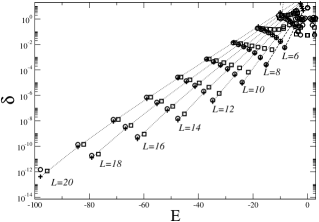
Figure 1: Energy splittings $\delta$ versus $E$ for the many–spin case. Eigenvalues and splittings are compared for the case $N=20$, $\eta=1$ and $l=1$. Circles : mean field approximation; squares : full Hamiltonian; crosses : perturbative result. Eigenvalues are arranged in regular block, according to different $L$ values as indicated in the figure.

In order to understand the origin of this regularities, it is useful to rewrite (1) as $\hat{H}=\hat{H}_{MF}+\hat{H}_{1}$, where

$$\hat{H}_{MF} = \frac{\eta}{2}\hat{m}_{x}^{2}-\frac{1}{2}\hat{m}_{y}^{2}$$ (2)

$$\hat{H}_{1} = \frac{1}{2}\sum(\hat{S}_{i}^{y})^{2}-\frac{\eta}{2}\sum(\hat{S}_{i}^{x})^{2}.$$ (3)

and $\hat{m}_{x,y,z}=\sum_{i}\hat{S}_{i}^{x,y,z}$. While the first term (mean field) is integrable in the classical limit, the latter is responsible for the non integrability of the system. Let us also consider the eigenvectors of $\hat{H}_{MF}$, $|E_{MF}\rangle$, and expand the eigenvectors of $\hat{H}$, $|E\rangle$ over them. In other words we consider the probability, $p_{0}=|\langle E_{MF}|E\rangle|^{2}$, that a given eigenvectors of $\hat{H}$ occupies a given eigenvector of $\hat{H}_{MF}$. As one can see, see Fig. 2a, the eigenvectors of the full Hamiltonian are almost completely localized on the eigenvectors of the mean field Hamiltonian. over the whole energy range. Actually in the low energy region the eigenvectors occupies just one eigenstate of the mean field Hamiltonian with probability greater the $0.9$, while all the other states are occupied with probability smaller the $0.01$. The same does not happen in the large $l$ case (Fig. 2b). Therefore, the non-integrable part is negligible with respect to the mean field (2). The question of the quantum integrability of chaotic Hamiltonians for bosons with $l=1$ has been recently posed in benet . Shortly, quantum integrability should be induced, for $l=1$, by the strong correlations between Hamiltonian matrix elements.

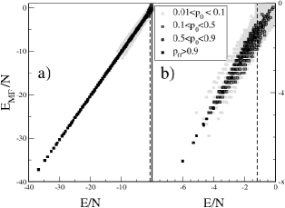
Figure 2: Probability $p_{0}=|\langle E|E_{MF}\rangle|^{2}$ that an eigenstate $|E\rangle$, with specific energy $E/N$, occupies an eigenstate $|E_{MF}\rangle$, with specific energy $E_{MF}/N$. Parameters are : a) $N=100$, $l=1$ ; b) $N=6$ $l=4$.

From the above analysis it follows that we can use the mean field Hamiltonian to study the total Hamiltonian in the hard quantum regime.

Here, we present the results of a high order perturbative calculation of the eigenvalues of $\hat{H}_{MF}$. Since $[\hat{H}_{MF},{\hat{m}^{2}}]=0$, it is sufficient to consider the eigenvalues of $\hat{m}^{2}$. They are given by the possible values of the total magnetic moment which can be obtained combining $N$ particles of spin $l$, and are determined by the quantum numbers: $Nl,Nl-1,....,0$. From these values we should exclude those which cannot be combined to give completely symmetric states, if one is interested in the bosonic case (even if the present approach is independent from the statistics). We can consider each subspace with different $m^{2}$ separately. In this way the many-spin Hamiltonian $\hat{H}_{MF}$, is equivalent to a set of single spin systems, described by the same Hamiltonian. Note that $l$ is the magnitude of the spin of the many-spin problem. Thus in the following we will first consider single spin models, and then we will come back to our many-spin problem.

III Single Spin Model

Let us consider a single spin of magnitude $L$, $z-$ component $L_{z}$, with $|L_{z}|\leq L$. For simplicity we will rewrite the mean field Hamiltonian as follows:

$$\hat{H}_{MF}=\frac{1}{2}\left(-\hat{m}_{z}^{2}+\eta\hat{m}_{x}^{2}\right)$$ (4)

Eq. (4) can be reduced to (3) after a rotation of $\pi$ around the $x$ axis which carries $y$ in $z$ and $z$ in $-y$, and does not affect the physics of the problem.

Single-spin-model have an interest in themselves, besides the fact that their analysis will allow us to compute the energy levels of our many-spin mean field Hamiltonian. In recent years growing interest arose in micromagnetic particles chud ; takagi , such as ferromagnetic domains and magnetic macro–molecules such as $Mn_{12}$ and $Fe_{8}$ molecule . The research interest in these systems is mainly due to the possibility to reveal quantum effects in the macroscopic domain, such as the Macroscopic Quantum Tunneling (MQT) of the magnetic moment, and the even more interesting phenomenon of Macroscopic Quantum Coherence (MQC). While in the former case (MQT) the total magnetization of a microscopic particle flip even if classically this would be forbidden by the presence of an effective energy barrier, in the latter case (MQC) the magnetization oscillates between opposite magnetization states in a coherent way. This phenomenon, if revealed, would unambiguously indicate the presence of Quantum Interference of Macroscopic Distinct States leggett . At sufficiently low energy these systems can be modeled by phenomenological single–spin Hamiltonians, where the single spin describes the total magnetic moment of the system. Splittings of the eigenvalues of the single spin Hamiltonians are simply related to the frequencies of MQC (or the tunneling rates of MQT) chud . For this reason much effort has been devoted in these years to compute such splittings. Usually, semiclassical methods are employed, such as WKB and imaginary time path integrals to quote but a few svizzeri ; chud2 . Also perturbation theory can be successfully applied in this kind of problem taking into account high order terms garanin . Indeed it is possible to compute explicitly the first non–zero perturbative contribution to the splittings even if this is an high–order contribution.

In Appendix V we show the basic ideas of the high perturbative order approach, and we derive an analytical expression for the eigenvalues and the corresponding splittings (in garanin no explicit derivation was given).

Numerical eigenvalues and their splittings for Hamiltonian (4) and a single spin of magnitude $L$, have been compared with our results in Fig. 3, where we show the splittings $\delta$ as a function of the energy $E$.

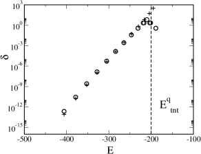
Figure 3: $\delta$ shifts versus the energy $E$. Eigenvalues and splittings obtained numerically (open circles) and via perturbation theory (crosses) for a single spin $L=20$. Also shown as vertical dashed line the rough estimates for the validity of the our approach. Here is $\hbar=1$, $\eta=-0.5$.

In the same figure we can see that while the high perturbative order approach gives a very good estimate for $E<E^{q}_{tnt}$ it fails completely above the threshold. An upper bound to the energy at which our approach fails can be given evaluating the quantum correction to $E_{tnt}$ for the single spin Hamiltonian, see bcb (indicated in Fig. 3 as a vertical dashed line).

IV Many spin Hamiltonian

We now compare our analytical results with the eigenvalues of the mean field Hamiltonian $H_{MF}$ considered as a many spin Hamiltonian and with the eigenvalues of the complete Hamiltonian in the hard quantum regime (1). We can achieve this by considering the possible eigenvalues of $\hat{m}^{2}$, which are obtained when an ensemble of $N$ particles of spin $l$ is considered. Note that from the set of possible eigenvalues of $\hat{m}^{2}$ we have to exclude those that are not compatible with the symmetrization postulate (for the bosonic case). For each possible value of $\hat{m}^{2}$ we apply our perturbative approach to the correspondent single spin problem. Then, putting all together, we obtain the results for the many–spin Hamiltonian.

In Fig. 1 we plot the splittings versus the specific energy for the mean field Hamiltonian (2) (circles), for the full Hamiltonian (1) (squares), and the perturbative results (crosses). As one can see we can give an accurate good approximation in the low energy region of the spectrum. Deviations obviously appear when the perturbative approach is compared with the splittings of the full Hamiltonian, even if, in this case, the perturbative approach still give a correct order of magnitude estimate of eigenvalues and splitting. From Fig. 1 we can also see how the regular features of $\delta$ in the hard quantum regime are related to the quantum numbers of the total angular momentum.

One could ask if the same perturbative approach works in the semiclassical regime for the total Hamiltonian (2). Perturbation theory cannot work in the whole energy region, even if we may expect to give an approximate description for low–energy eigenvalues. For instance, applying perturbation theory, e.g. Eq. (14), for the energy separation between the ground state and the first excited state, we get: $\delta_{GS}=0.25\hbar^{2}/6^{-Nl}$. This expression works works fairly wellcelardo , even for large $l$ and it reproduces the main features of the dependence of the ground state splitting, namely the exponential dependence on $l$, and $N$ as well.

We have shown that, in the hard quantum regime, it is possible to compute perturbatively the splittings of the doublets characterizing the spectrum below the quantum TNT. This is due to the nearness of the full Hamiltonian with the mean field Hamiltonian. The quantum TNT can be also considered a perturbative threshold, since it gives an estimate of the energy at which the perturbative approach fails. Finally, we point out that this threshold indicates an energy range which is not negligible with respect to the total energy range for long range interacting systems in which Macroscopic Quantum Phenomena can be studied.

V Appendix

In this section we present the results of a high perturbative order calculation of the eigenvalues of the single spin Hamiltonian (4). We will show that in order to split the double degenerate levels of the $-\hat{m}_{z}^{2}$ term of (4) characterized by the quantum number $l_{0}=|m_{z}|$, the first non–zero contribution is at the $l_{0}$-th perturbative order. This also give a qualitative explanation of the well known exponential dependence of the splitting magnitudes on the energy.

Let us consider a single spin of magnitude $L$, $z$-component $L_{z}$ with $|L_{z}|\leq L$ and $|L,L_{z}\rangle$ as basis states. Hamiltonian (4) can be written as $\hat{H}=\hat{H}_{0}+\hat{V}$, where :

$$\hat{H}_{0} = -\hat{m}_{z}^{2}+\frac{1}{4}\eta(\hat{m}^{+}\hat{m}^{-}+\hat{m}^{-}\hat{m}^{+})$$

$$\hat{V} = \frac{1}{4}\eta(\hat{m}^{+}\hat{m}^{+}+\hat{m}^{-}\hat{m}^{-})$$ (5)

and $\hat{m}^{\pm}=\hat{m}_{x}\pm i\hat{m}_{y}$. Since $\hat{H}_{0}$ is diagonal in the basis $|L,L_{z}\rangle$, the unperturbed energy $E_{0}=\langle L,l_{0}|\hat{H}|L,l_{0}\rangle$ are given by:

$$E_{0}(L,l_{0})=-\hbar^{2}l_{0}^{2}+\frac{1}{2}\hbar^{2}\eta\left[L(L+1)-l_{0}^{2})\right]$$ (6)

Each unperturbed energy level turns out to be doubly degenerate, with eigensubspaces spanned by $|L,\pm l_{0}\rangle$. The first non-zero contribution to the splitting of a degenerate pair occurs at the $l_{0}$-th order of perturbation theory. In order to show that let us define the $n-$th order perturbation operator sakurai :

$$\hat{\cal P}^{(n)}=\hat{V}\left(\frac{\hat{\phi}}{E_{0}-H_{0}}\hat{V}\right)^{n-1},$$ (7)

where $\hat{\phi}=1-\sum_{{E^{\prime}}_{0}\neq E_{0}}|{E^{\prime}}_{0}\rangle\langle{E^{\prime}}_{0}|$ is the projector out of the considered degenerate subspace. The right linear combination of the unperturbed basis vectors $|L,\pm l_{0}\rangle$ (to which eigenstates of $\hat{H}$ tend when $\hat{V}$ is negligible) can be found by diagonalizing the following matrix:

$$\pmatrix{{\cal P}_{++}^{(n)}&{\cal P}_{+-}^{(n)}\cr{\cal P}_{-+}^{(n)}&{\cal P}_{--}^{(n)}}$$ (8)

where ${\cal P}_{ss^{\prime}}^{(n)}=\langle L,sl_{0}|\hat{{\cal P}}^{(n)}|L,s^{\prime}l_{0}\rangle$, $s,s^{\prime}=\pm 1$ and $n$ is the minimum order giving rise to two different eigenvalues of the matrix (8). A $\pi-$rotation around the $x-$axis leaves $\hat{V}$ unchanged since $|L,l_{0}\rangle\to|L,-l_{0}\rangle$, and $\hat{m}^{\pm}\rightarrow\hat{m}^{\mp}$. Then ${\cal P}^{(n)}_{++}={\cal P}^{(n)}_{--}$, ${\cal P}^{(n)}_{+-}={\cal P}^{(n)}_{-+}$ and the right combination of unperturbed basis vectors is:

$$|\pm m_{0}\rangle=(|L,l_{0}\rangle\pm|L,-l_{0}\rangle)/\sqrt{2}.$$ (9)

Eigenvalues undergo a shift given by : $\pm{\cal P}_{+-}^{(n)}$. The generic $n$-th order energy shift, $\Delta^{(n)}$ induced by the perturbation is given by: $\Delta^{(n)}=\langle\pm m_{0}|\hat{\cal P}^{(n)}|\pm m_{0}\rangle$. While the degeneracy can be removed only by non-zero off-diagonal elements, an overall energy shift $D$ can be induced by non-zero diagonal elements too.

In order to compute $D$ and $\delta$ the action of $\hat{\cal P}^{(n)}$ on the basis states $|L,\pm l_{0}\rangle$ should be evaluated. If $n=1$ then $\hat{\cal P}^{(1)}=\hat{V}$. In this case the diagonal elements of the matrix (8) are zero since $\hat{V}$ can only change $l_{0}\to l_{0}\pm 2$. Off–diagonal elements $\langle L,-l_{0}|\hat{V}|L,+l_{0}\rangle$ are different from zero only when $\hat{V}$ brings $|L,l_{0}\rangle$ into $|L,-l_{0}\rangle$. This can happen only if $l_{0}=1$.

If $n=2$ then $\hat{\cal P}^{(2)}=\hat{V}(\hat{\phi}/(E_{0}-H_{0}))\hat{V}$. Since

$$\frac{\hat{\phi}}{(E_{0}-H_{0})}|L,l\rangle=\frac{1-\delta_{l,l_{0}}}{E_{0}(L,l_{0})-E_{0}(L,l)}|L,l\rangle,$$ (10)

in order to understand the action of $\hat{\cal P}^{(2)}$ we have to apply $\hat{V}$ twice. Let’s consider the diagonal elements: Can we take $|L,l_{0}\rangle$ in itself $|L,l_{0}\rangle$, using $\hat{V}$ twice? Yes: $\hat{V}\hat{V}|L,l_{0}\rangle\rightarrow\hat{V}(|L,l_{0}-2\rangle+|L,l_{0}+2\rangle)\rightarrow|L,l_{0}\rangle+|L,l_{0}-4\rangle+|L,l_{0}+4\rangle+|L,l_{0}\rangle$, where the coefficients in front of the states have been omitted. Bracketing the final states thus obtained with $|L,l_{0}\rangle$, only the first and the last remain. Then there are two “ways” in which the operator $\hat{\cal P}^{(2)}$ can take $|L,l_{0}\rangle$ in itself: if $l_{0}>1$ by the following chain rule : $|L,l_{0}\rangle\rightarrow|L,l_{0}-2\rangle\rightarrow|L,l_{0}\rangle$, while if $l_{0}<L-1$ by $|L,l_{0}\rangle\rightarrow|L,l_{0}+2\rangle\rightarrow|L,l_{0}\rangle$.

It is now easy to compute the first non zero contributions to the overall shift. From (9) we have:

$$D=\langle L,\pm l_{0}|\hat{V}\left(\frac{\hat{\phi}}{E_{0}-H_{0}}\hat{V}\right)|L,\pm l_{0}\rangle,$$ (11)

The only contributions $D_{\pm}$ different from zero, coming from the two ways described above, are:

$$D_{\pm}=\left(\frac{\displaystyle\eta\hbar}{\displaystyle 4}\right)^{2}\frac{\displaystyle f^{\pm}(L,l_{0})f^{\pm}(L,l_{0}-1)}{\displaystyle\Delta E_{0}^{\pm}},$$ (12)

respectively for $l_{0}>1$ ($D_{-}$) and $l_{0}<L+1$ ($D_{+}$). Here, we defined $f^{\pm}(L,l_{0})=L(L+1)-l_{0}(l_{0}\pm 1)$ and $\Delta E_{0}^{\pm}=E_{0}(L,l_{0})-E_{0}(L,l_{0}\pm 2)$. Thus, $D=D_{-}+D_{+}$ is the first non–zero overall energy shift.

Let us now consider the off-diagonal matrix elements. It is possible to go from $|L,l_{0}\rangle$ to $|L,-l_{0}\rangle$ using $\hat{V}$ twice only when $l_{0}=2$. In this case there is one only way: $|L,l_{0}\rangle\rightarrow|L,l_{0}-2\rangle\rightarrow|L,l_{0}-4\rangle=|L,-l_{0}\rangle$, the last being true only for $l_{0}=2$. It is then clear why the first non-zero operator which splits the doublet characterized by $L,l_{0}$ is the $l_{0}$-th order. From (9) we have:

$$\delta=2\langle L,l_{0}|\hat{V}\left(\frac{\hat{\phi}}{E_{0}-H_{0}}\hat{V}\right)^{l_{0}-1}|L,-l_{0}\rangle$$ (13)

From Eq. (13) there is only one way to connect $|L,l_{0}\rangle$ with $|L,-l_{0}\rangle$, namely $|L,l_{0}\rangle\rightarrow|L,l_{0}-2\rangle......\rightarrow|L,-l_{0}+2\rangle\rightarrow|L,-l_{0}\rangle$. After some algebra, one has:

$$\delta=\hbar^{2}\left(\frac{\eta}{4}\right)^{l_{0}}(-1)^{l_{0}-1}\frac{\prod_{j=-l_{0}}^{l_{0}-1}\sqrt{L(L+1)-j(j+1)}}{\prod_{p=1}^{l_{0}-1}(4+2\eta)p(l_{0}-p)}$$ (14)

To summarize, for any given degenerate doublet we can calculate the overall shift $D$, Eqs.(12) and the splitting $\delta$, Eq.(14).

References

- (1) E. M. Chudnovsky and J. Tejada, Macroscopic Quantum Tunneling of the Magnetic Moment, Cambridge University Press, (1998).
- (2) M. Hartmann, G. Mahler and O. Wess. Phys. Rev. Lett. 93, 80402 (2004).
- (3) J. Barré, D. Mukamel, S. Ruffo, Phys. Rev. Lett. 87, 3, (2001).
- (4) J. Barré, F. Bouchet, T. Dauxois, and S. Ruffo, Phys. Rev. Lett. 89, 110601, (2002); T. Dauxois, S. Ruffo, E. Arimondo, M. Wilkens Eds.,Lect. Notes in Phys., 602, Springer (2002).
- (5) F. Borgonovi, G. L. Celardo, M. Maianti, E. Pedersoli, J. Stat. Phys., 116, 516 (2004).
- (6) R. G. Palmer, Adv. in Phys., 31, 669 (1982).
- (7) A. I. Khinchin Mathematical Foundations of Statistical Mechanics, Dover Publications, New York (1949).
- (8) A. J. Leggett and A. Garg, Phys. Rev. Lett. 54, 857 (1985), A. J. Leggett, J. Phys., 14, R415-R451 (2002), A. J. Leggett, Rev. Mod. Phys. 59, 1, (1987).
- (9) F. Borgonovi, G.L. Celardo, A. Musesti, and R. Trasarti-Battistoni cond-mat/0505209.
- (10) G.L.Celardo, J.Barré, F.Borgonovi, S. Ruffo, cond-mat/04010119.
- (11) F. Borgonovi, G. L. Celardo, and G. P. Berman, cond-mat/0506233.
- (12) L. Benet, T. Rupp and H. A. Weidenmuller, Phys. Rev. Lett. 87, 010601 (2001); T. Asaga, L. Benet, T. Rupp and H. A. Weidenmuller, Europhys. Lett. 56, 340 (2001); T. Asaga, L. Benet, T. Rupp and H. A. Weidenmuller, Ann. of Phys. 298 229 (2002).
- (13) S.Takagi, Macroscopic Quantum Tunneling, Cambridge University Press, (1997).
- (14) J. Schnack, cond–mat/0501625.
- (15) M.Enz and R.Schilling, J.Phys. C, 19, 1765-1770 (1986), M.Enz and R.Schilling, J.Phys. C, 19, L711-L715 (1986), G.Scharf, W.F.Wreszinski and J.L.Hemmen, J.Phys. A, 20, 4309-4319 (1987).
- (16) E.M.Chudnovsky and L. Gunther, Phys. Rev. Lett. 60, 611 (1988).
- (17) D.A. Garanin, J. Phys. A 24, L61-L62 (1991).
- (18) G. L. Celardo, PhD dissertation , University of Milan, Italy (2004).
- (19) J.J. Sakurai, Modern Quantum Mechanics, Addison-Wesley Publishing Company (1985).