Estimation of critical behavior from the density of states in Classical Statistical Models

Abstract

We present a simple and efficient approximation scheme which greatly facilitates extension of Wang-Landau sampling (or similar techniques) in large systems for the estimation of critical behavior. The method, presented in an algorithmic approach, is based on a very simple idea, familiar in statistical mechanics from the notion of thermodynamic equivalence of ensembles and the central limit theorem. It is illustrated that, we can predict with high accuracy the critical part of the energy space and by using this restricted part we can extend our simulations to larger systems and improve accuracy of critical parameters. It is proposed that the extensions of the finite size critical part of the energy space, determining the specific heat, satisfy a scaling law involving the thermal critical exponent. The method is applied successfully for the estimation of the scaling behavior of specific heat of both square and simple cubic Ising lattices. The proposed scaling law is verified by estimating the thermal critical exponent from the finite size behavior of the critical part of the energy space. The density of states (DOS) of the zero-field Ising model on these lattices is obtained via a multi-range Wang-Landau sampling.

I Introduction

In the past half-century, importance sampling in the canonical ensemble and especially the Metropolis method and its variants was the main tool in condensed matter physics, mainly for the study of critical phenomena metro53 ; glaub63 ; bortz75 ; binde77 ; newma99 ; landa00 . However, this standard approach has two serious disadvantages. The partition function of the statistical model is not an output of such calculations and in many cases importance sampling is trapped for significant time in valleys of rough free energy landscape. Over the last decade, there have been a number of interesting approaches addressing to these problems newma99 ; landa00 ; lee93 ; berg92 ; ferre98 ; lima00 ; wang02 ; wang99 ; wang01 ; wang01b . Recently efficient methods that directly calculate the density of states (DOS), or the spectral degeneracy, of classical statistical models have been developed. A few remarkable examples are the entropic newma99 ; lee93 , multicanonical berg92 , histogram and broad histogram ferre98 ; lima00 , transition matrix wang02 ; wang99 and Wang-Landau wang01 ; wang01b ; schul03 ; schul01 ; landa02 methods. The above methods are thought to be the most promising ones for the application of finite-size analysis in data with higher accuracy. It is well known landa00 that finite-size analysis is very sensitive to simulational errors and in most cases the asymptotic analysis may become a notorious task, due to the fact that these errors may “interfere” with unknown correction terms landa00 .

In this paper we concentrate on the Wang-Landau method wang01 ; wang01b ; schul03 ; schul01 ; landa02 . Noteworthy that this method was applied by these authors on the two-dimensional Ising model producing the density of states even on lattices, as large as, $256\times 256$. This was achieved by a multi-range algorithm in which independent random walks were used for different energy subintervals and the resultant pieces were then combined to obtain the density of states. The possibility of producing accurate estimates for critical-point anomalies on large lattices establishes, at least it is hoped, Wang-Landau method, and similar techniques, as new and important tools for evaluating equilibrium properties of models showing complex properties of substances, such as systems with competing interactions and spin glass models. Therefore, it is of interest to understand how we can implement these methods in the best way for the extraction of critical parameters using the finite-size scaling theory. This paper considers an important aspect of this problem and aims to introduce a simple and practical route, through which we can substantially improve both accuracy and efficiency of the above methods. It will be shown that only a relatively small part of spectral degeneracies is needed in order to obtain a good estimation of critical properties. This part of the total energy range can be easily identified. In Section II we present an outline of the method which one can use to identify the subspace of the energy space that determines the specific-heat peak behavior. Also a very brief description of the multi-range Wang-Landau method is presented. In Section III the proposed method is tested for the plane square Ising lattice where the finite-size scaling behavior is known from the work of A. Ferdinand and M. Fisher ferdi69 . In Section IV we discuss the critical-point specific heat anomaly behavior of the simple cubic Ising lattice. We present estimates for the critical temperature and the associated critical exponents and compare our results with existing estimates. It is shown that the extension of the used critical energy subspace scales as predicted in the theory presented in Section II and this provides an independent estimation of the ratio $\alpha/\nu$ of critical exponents. We summarize our results and conclusions in Section V.

II Estimation of the critical part of the energy space

Let us consider the zero-field Ising model on the $L\times L=N$ square and the $L\times L\times L=N$ cubic lattices:

$$H=-J\sum_{<ij>}S_{i}S_{j},\;\;\;\;S_{i}=\pm 1,\;\;\;\;i=1,2,...,N$$ (1)

The behavior of finite systems near the infinite lattice critical temperature $T_{c}$ can be described by finite-size scaling theoryfishe71 ; privm90 ; binde92 . For the three dimensional Ising model the maxima of the finite-size specific heats $C^{\ast}_{L}$ are expected to scale as:

$$C^{\ast}_{L}=c+bL^{\alpha/\nu}(1+...)$$ (2a)

Where $$\alpha \nu C^{\ast}_{L} T^{\ast}_{L}$$ and are the critical exponents of the specific heat and the correlation length, respectively. For the square Ising lattice the (logarithmic) scaling of the maxima of the finite-size specific heats is known from the work of A. Ferdinand and M. Fisher ferdi69 and will be considered in the next section. The shift of the “pseudo-critical” temperatures (defined by the location of the specific-heat peaks) is described by a similar power law for both square and cubic Ising lattices:

$$T^{\ast}_{L}=T_{c}+cL^{-1/\nu}(1+...)$$ (2b)

Given an approximation for the density of states, $G(E)$, obtained for instance via the Wang-Landau method, the specific heat at any temperature can be estimated and thus the“pseudo-critical” temperature $T_{L}^{\ast}$ and the maximum of the specific heat are easily obtained. Therefore, applying such a method to finite systems, we can accumulate data and through the finite size scaling mechanism extract the asymptotic critical behavior. Of course, this has been done in the past using the more traditional Monte Carlo methods (particularly importance sampling techniques). Using these later methods we have to simulate the system in a range of temperatures around the “pseudo-critical” temperature $T^{\ast}_{L}$. For each such temperature we have to perform our simulations for a suitably long period of time for “equilibration” and then make a large number of independent measurements for averaging. In effect, this usually means a very large number (several millions) of Monte Carlo steps determined mainly by the critical slowing down phenomenon newma99 ; landa00 . On the other side, using the Wang-Landau method one has “at once” an approximation of the specific heat at any temperature and thus, as mentioned above, the “pseudo-critical” temperature $T^{\ast}_{L}$ and the maximum of the specific heat are easily obtained. However, executing a Wang-Landau random walk process in the total energy space can also be time-consuming and moreover the almost unavoidable multi-range algorithm will definitely introduce some “uncontrollable” errors. These errors are “histogram errors” which may propagate and amplify through the process of connecting the energy ranges in a multi-range approach. Note that by applying separately a histogram flatness criterion (such as (11)) in each energy range does not produce necessarily the same level of flatness in the total energy range. It is therefore profitable if we can estimate, with the same or even better accuracy, the specific heat peaks using only a small part of the energy space.

In order to proceed we express the value of the specific heat, at any temperature, with the help of the usual statistical sum $(k_{B}=1)$:

$$C_{L}(T)=N^{-1}T^{-2}\left\{Z^{-1}\sum^{E_{max}}_{E_{min}}E^{2}\exp[{\Phi(E)}]-\left(Z^{-1}\sum^{E_{max}}_{E_{min}}E\exp[{\Phi(E)}]\right)^{2}\right\}$$ (3a)

where $$\Phi(E) S(E)$$ and the microcanonical entropy are defined by:

$$\Phi(E)=S(E)-\beta E,\;\;\;S(E)=\ln{G(E)}$$ (3b)

while the function Z by:

$$Z=\sum_{E_{min}}^{E_{max}}\exp{[\Phi(E)]}$$ (3c)

Note that $Z$ is the partition function in case one uses the total energy spectrum and $G(E)$ is properly normalized. The above expressions give, in fact, an approximation for the values and the maximum of the specific heat since Wang-Landau simulations provide us with an approximate DOS $G(E)$.

Now let $\widetilde{E}$ denote the value of energy producing the maximum term in the sum (3c) of the (partition) function at a temperature of our interest. Eventually, we will concentrate on the “pseudo-critical” temperature $T_{L}^{\ast}$ or some temperatures close to this (for instance the exact critical temperature $T_{c}$, whenever this temperature is known). We may define a set of approximations to the specific-heat values by restricting the statistical sums in (3) to energy ranges around this value. We define the following energy sub-ranges of the total energy range ($E_{min},E_{max}$):

$$(\widetilde{E}_{-},\widetilde{E}_{+}),\;\;\;\;\widetilde{E}_{\pm}=\widetilde{E}\pm\Delta^{\pm},\;\;\;\;\;\Delta^{\pm}\geq 0$$ (4)

Accordingly, the value of the specific heat at the temperature of interest (for instance, the value of the peaks at the“pseudo-critical” temperature $T^{\ast}_{L}$ ) are approximated by:

$$C_{L}(\widetilde{E}_{-},\widetilde{E}_{+})\equiv C_{L}(\Delta^{\pm})=N^{-1}T^{-2}\left\{\widetilde{Z}^{-1}\sum_{\widetilde{E}_{-}}^{\widetilde{E}_{+}}E^{2}\exp{[\widetilde{\Phi}(E)]}\right.\\ \left.-\left(\widetilde{Z}^{-1}\sum_{\widetilde{E}_{-}}^{\widetilde{E}_{+}}E\exp{[\widetilde{\Phi}(E)]}\right)^{2}\right\}$$ (5a)

where

$$\widetilde{\Phi}(E)=[S(E)-\beta E]-\left[S(\widetilde{E})-\beta\widetilde{E}\right]$$ (5b)

and

$$\widetilde{Z}=\sum_{\widetilde{E}_{-}}^{\widetilde{E}_{+}}\exp{[\widetilde{\Phi}(E)]}$$ (5c)

Depending on the extension of the sub-ranges used in (5) the above sequence may give good approximations to the specific heat values.

As mentioned earlier, finite-size analysis depends on the accuracy of the finite lattice data, in a very sensitive way. Therefore, one may question the utility of introducing further approximations to an already approximate scheme. To answer this we demand that the new errors are much smaller than the already existing ones from the DOS approximation. Since by definition $\widetilde{\Phi}(E)$ is negative we can easily see that for large lattices “extreme” values of energy (far from $\widetilde{E}$) will have an extremely small contribution to the statistical sums since these terms decay exponentially fast with respect to the distance from $\widetilde{E}$. It follows that, if we request a specified accuracy (assume that our approximations satisfy some strict criteria), then we may greatly restrict the necessary energy range, in which DOS should be sampled. If this is so, then we not only reduce computer time for the calculation of the approximate DOS, but we also improve accuracy. Indeed, by restricting the energy space we should expect a minimization of “Wang-Landau errors” even in cases where a multi-range approach is used.

To make this idea concrete we demand that the relative errors introduced by the restriction (5) are smaller than a given number r. Moreover we assume that these relative errors are considerably smaller than those produced by the Wang-Landau scheme on the values of the specific heat. This restriction is well defined if we know the exact DOS for a finite system. Given any small number and the exact DOS one can easily calculate the minimum energy subspace (MES), compatible with the above restriction. An algorithmic approach is described below in equations (9). The resulting subspace (its end-points and its extension) depends, of course, on the temperature, on the value of the small parameter r, and on the lattice size. We write for its extension, $\Delta\widetilde{E}$:

$$\Delta\widetilde{E}\equiv\Delta\widetilde{E}(T,\textit{r},L)\equiv min(\widetilde{E}_{+}-\widetilde{E}_{-}):$$

$$\mid\frac{C_{L}(\Delta^{\pm})}{C_{L}}-1\mid\leq\textit{r}$$ (6)

Closely related to the notion of the thermodynamic equivalence of ensembles and to the central limit theorem is here the idea that, for any temperature, the extension of the energy subspace determining the behavior of the system is much smaller than the total energy range: $\Delta\widetilde{E}(T,\textit{r},L)\ll(E_{max}-E_{min})$. Thus, our proposition of using Wang-Landau sampling in the critical MES is quite obvious. We should expect that the extension of the above-defined restricted part of the energy space would be of the same order with the standard deviation of the energy distribution at any temperature. Therefore, we assume that given a small constant value for r:

$$\Delta\widetilde{E}\propto\sigma_{E}=\sqrt{NT^{2}C}$$ (7)

From the central limit theorem we know that, far from the critical point, the energy distribution approaches a Gaussian distribution and the energy subspace determining all thermodynamic properties is mostly of the order of $\sqrt{N}$. Close to a critical point the order of the extension of MES is not known, but assuming thermodynamic equivalence of ensembles one should expect the extension of critical MES to be $\ll N$ . Although the energy distribution will diverge from the Gaussian, it still seems reasonable to describe the extensions of the critical MES, $\Delta\widetilde{E}^{\ast}=\Delta\widetilde{E}(T^{\ast}_{L},\textit{r},L)$ by (7). Therefore, using (2a) we may conclude that these extensions, as well as the values $\Delta\widetilde{E}_{c}=\Delta\widetilde{E}(T_{c},\textit{r},L)$, should scale as:

$$\frac{\Delta\widetilde{E}^{\ast}}{L^{d/2}}\approx L^{\frac{\alpha}{2\nu}}$$ (8)

In order to obtain the MES from the exact DOS or from a given approximation of DOS, $G(E)$, we define successive ‘minimal’ approximations to the specific-heat values:

$$C_{L}(j)\equiv C_{L}(\Delta_{j}^{-},\Delta_{j}^{+}),$$

$$\Delta^{\pm}_{j+1}=\Delta^{\pm}_{j}\pm\theta^{\pm}_{j+1},\;\;\ \Delta_{1}^{\pm}=0,\;\;\;\ j=1,2,...$$ (9a)

One of the above $\theta$-increments is chosen to be 1 and the other 0 according to which side of $\widetilde{E}$ is producing at the current stage the best approximation:

$$(\theta^{+}_{j+1}=1,\theta^{-}_{j+1}=0)\;\Leftrightarrow$$

$$\mid C_{L}-C_{L}(\Delta_{j}^{-},\Delta^{+}_{j}+1)\mid\leq$$

$$\leq\mid C_{L}-C_{L}(\Delta_{j}^{-}+1,\Delta_{j}^{+})\mid\;$$ (9b)

$$(\theta^{+}_{j+1}=0,\theta^{-}_{j+1}=1)\;\Leftrightarrow$$ (9c)

$$\mid C_{L}-C_{L}(\Delta_{j}^{-},\Delta^{+}_{j}+1)\mid>$$

$$>\mid C_{L}-C_{L}(\Delta_{j}^{-}+1,\Delta_{j}^{+})\mid$$

Accordingly the sequence of relative errors for the specific-heat values ($\textit{r}_{j}$) is given by:

$$\textit{r}_{j}=\mid\frac{C_{L}(j)}{C_{L}}-1\mid$$ (9d)

We now fix our requirement of accuracy by specifying a particular level of accuracy for all finite lattices. In effect, we define the (critical) MES as the subspace centered at $\widetilde{E}$ ($\widetilde{E}^{\ast}$) corresponding to the first member of the above sequence (9) satisfying: $\textit{r}_{j}\leq\textit{r}$. Demanding the same level of accuracy for all lattice sizes, we produce a size-dependence on all parameters of the above energy ranges. That is we should expect that the “center” $\widetilde{E}(T,L)$ and the end-points $E_{-}(T,r,L)$, $E_{+}(T,r,L)$ of the (critical) MES are all functions of L. In particular the extensions $\Delta\widetilde{E}^{\ast}=\Delta\widetilde{E}(T_{L}^{\ast},\textit{r},L)$ of the critical MES should obey the scaling law (8). It is therefore possible to find approximations of these functions using the total energy range for small lattices and then extrapolate to estimate the critical MES for larger lattices. A slightly wider energy subspace is easily predicted by extrapolating from smaller lattices. Furthermore, working in a wider range we can use our approximate DOS to have a very good approximation of the critical MES and thus check the validity of the proposed scaling law (8). This is possible, because, the approximations are expected to obey an exponentially fast convergence outside the energy range centered in $\widetilde{E}$. We may also apply the above r-depended scheme for several values of the accuracy parameter r. Once the accuracy criteria have been satisfied for a given value of r and the energy range is wide enough to accurately estimate the corresponding CrMES, we can also estimate the extensions of CrMES for any larger value of the parameter r.

Let us now briefly discuss the main points of our implementation of the Wang-Landau method. For the application of the algorithm in multi-range approach we follow the description of Schulz et al. $2003$, i.e., whenever the energy-range is restricted we use the updating scheme $2$ described in that paper. Consider the restriction of the random walk in a particular energy-range $I=[E_{1},E_{2}]$ and assume that the random walk is at the border of the range I. Then, the next spin-flip attempt is determined by the modified Metropolis acceptance ratio:

$$A=\left\{\begin{array}[]{rr}\min\{1,G(E)/G(E+\Delta E)\},&\mbox{$(E+\Delta E)\in I$}\\ 0,&\mbox{$(E+\Delta E)\not\in I$}\end{array}\right.$$ (10)

The random walk is not allowed to move outside of the energy range, and we always update the histogram value $H(E)\rightarrow H(E)+1$ and the DOS value $G(E)\rightarrow G(E)^{\ast}\textit{f}_{j}$ after a spin-flip trial. Here, of course, $\textit{f}_{j}$ is the value of the Wang-Landau modification factor wang01 ; wang01b ; schul03 ; schul01 ; landa02 , at the $j^{th}$ iteration, in the process ($\textit{f}\rightarrow\textit{f}^{\,1/2}$) of reducing its value to 1, where the detailed balance condition is satisfied. In all our simulations the Wang-Landau modification (or the control parameter), was chosen to have the initial value: $\textit{f}_{j=1}=e\approx 2.71828...$. When starting a new iteration the control parameter is changed according to $\textit{f}_{j+1}=\sqrt{\textit{f}_{j}},j=1,2,...$ wang01 . Also, we use the following criterion for the histogram flatness:

$$\frac{maxH(E)-minH(E)}{maxH(E)}\leq 0.05$$ (11)

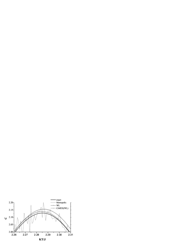
Figure 1: Comparative diagram showing the exact specific heat (in units of $k_{B}$) for a $50\times 50$ square Ising lattice (solid line) and approximate curves corresponding to (i) Metropolis Importance sampling. Average behavior over $20$ samples. For each temperature we have used after equilibration about $\sim 10^{4}$ Monte Carlo sweeps for averaging. (ii) Wang-Landau multi-range sampling ($4$ independent random walks transversing the total energy range. (iii) Wang-Landau multi-range sampling applied to the critical energy subspace (CrMES) (i.e. $20$ independent random walks ran in a slightly wider energy range of extension $\sim 450$ energy levels). Note that (ii) and (iii) have approximately the same time requirements. Obviously the improved accuracy of the proposed scheme is apparent mainly because, for the same available time, one can perform more independent WL random walks.

Using a multi-range approach, we divide the total energy range or the expected MES in several subintervals overlapping in one or several points at their ends. These subintervals can be then joined at the end to obtain the DOS in the range of interest. In joining two neighboring subintervals the degeneracies in one of the two have to be adjusted so that its endpoint degeneracies conform to the corresponding degeneracies of the neighboring interval. Obviously, this is a process that may propagate “histogram errors”, but from the description above it is apparent that one can arrange this process to leave unchanged the “central subinterval degeneracies”. Since this subinterval can be chosen to have its center close to the energy value $\widetilde{E}(T^{\ast}_{L})$, this choice will be optimal and it will produce relatively small errors. Usually, when one is sampling the total DOS, a normalization condition is applied. This condition may concern the ground state degeneracy, or the total number of states of the system, or even some convenient combination of known degeneracies. However, normalization does not effect the values of the specific heat, so we may conveniently choose $G(\widetilde{E}^{\prime})=1$, where $\widetilde{E}^{\prime}$ is an initial guess for $\widetilde{E}(T_{L}^{\ast})$ which serves as the center of the “central subinterval”. Furthermore, since the central subinterval is the most influential in the determination of the specific-heat peak, we have chosen the subintervals to have varying lengths(of the order of $50-160$ energy levels) with the largest to be the central subinterval ($100-160$ energy levels). Finally, in each case we observed the behavior in a sample of several independent runs and the j-iteration process ($\textit{f}_{j+1}=\sqrt{\textit{f}_{j}},j=1,2,...$) is carried out, until fluctuations around a ‘mean’ for the specific-heat peak are obtained. In almost all cases, this occurred in the range between $20-26$ Wang-Landau iterations for the modification factor. Fig.1 shows the application of Monte Carlo approaches to the specific heat peak for a $50\times 50$ square Ising lattice. The traditional Metropolis importance sampling, the Wang-Landau multi-range sampling of the total DOS and the proposed in this paper “critical minimum energy subspace (CrMES)” sampling are compared to the exact specific-heat peak.

III A Test Case: The Square Ising Lattice

A. Ferdinand and M. Fisher ferdi69 have asymptotically analyzed the critical point anomaly of a $\textit{m}\times\textit{n}$ plane square Ising lattice with periodic boundary conditions. In that paper, which has been one of the most influential papers in the development of finite-size scaling theory, an explicit expansion for the specific heat close to the critical point is described. We shall use their asymptotic expansion to test our simulational data obtained via Wang-Landau scheme in the CrMES. This is a first examination of our proposal for estimating the critical behavior through a “CrMES Wang-Landau scheme”. Furthermore, by performing the Wang-Landau random walk in a slightly wider range than the CrMES, we can estimate the finite-size extensions of the CrMES and explore the possibility of estimating the critical behavior using the scaling law proposed in (8).

Since for the two-dimensional case the exact critical temperature $T_{c}$ is known, it is useful to apply the “CrMES Wang-Landau scheme” for both the exact critical temperature and the “pseudo-critical” temperature $T^{\ast}_{L}$. Actually, this means that we have to run the Wang-Landau random walk in a wider range. As an example, let us give details for the case of a $50\times 50$ lattice. Counting the energy levels as $ie(E)=(E+2N)/4+1$, that is starting the enumeration from the ground state, the energy levels corresponding to the “centers” for the two temperatures of interest are $ie(\widetilde{E}(T_{c}))=354$ and $ie(\widetilde{E}(T_{L}^{\ast}))=378$. The corresponding extensions for a chosen level of accuracy $\textit{r}=10^{-6}$ are $392$ and $394$ respectively. Note that these ‘extensions’ are measured in terms of the convenient counting integer variable $ie(E)$. The extensions of the critical ranges are of the same order but their “centers” do not coincide (reflecting the shift of the “pseudo-critical” temperature). Their displacement is $24$ energy levels, so in order to achieve (for the specific-heat approximation (5)) a relative error of the order of $\textit{r}=10^{-6}$, we should execute the Wang-Landau random walk in a range of the order of $420$ $(394+24)$ energy levels. If we furthermore request to accurately estimate the extensions of the corresponding MES, we should consider a slightly wider (from each side) range, which in the case of a $50\times 50$ lattice modifies the required range of the order of $450$ energy levels. Thus, the number of energy levels for the Wang-Landau random walk is greatly reduced, since this number should be compared to a total of $2500$ energy levels for the $50\times 50$ lattice. A practical method for guessing the wider range necessary for an accurate estimation of the extensions of the CrMES may be as follows. We can easily devise a “self-consistent” test to inspect from the derived DOS (in the wider range) whether or not the estimated critical extensions are completely determined in this wider range. This is easily accomplished by using successively increasing ranges, starting from the estimated CrMES ranges, and observing the variation in the estimated extensions as the range grows up to the final wider version. Because of the exponential convergence mentioned earlier, this procedure will converge very fast. Thus, one can manage to know after his runs whether the originally “guessed” (or estimated through an extrapolation scheme) range was large enough to produce accurately the extensions of CrMES. After a successful run for a given lattice size we may know, if we wish, to what percentage was necessary to increase the CrMES (from each side) in order to accurately estimate its extension. This information may be then used for extrapolation to larger lattice sizes.

Table 1 presents the “pseudo-critical” temperatures, the corresponding values of the specific heats as well as the values of the specific heats at the exact critical temperature for lattice sizes $L=10-100$. The results for $L=10-50$ were obtained using the exact DOS derived by executing the algorithm provided by beale96 , while the estimates for the larger lattices by the proposed CrMES Wang-Landau scheme. For the lattice $50\times 50$ both exact and approximate results are shown for comparison. For each lattice size we have considered $20$ random walks in order to improve statistics. To obtain estimates of the errors, the specific-heat values were calculated separately from the DOS of each random walk (thus taking afterwards suitable averages), but also from the averaged DOS of the sample. We have also observed the variation of the estimated parameters as a function of the order of Wang-Landau iteration in the process of reducing the modification factor. Although we do not know any general criterion for an ‘optimum’ estimation using the Wang-Landau technique, we think it is a good practice to observe the variation of the estimated parameters as we proceed in higher orders of the approximate scheme. The errors given in brackets reflect the order of the standard deviation of averaging the separate walk estimates. Of course, using groups of random walks one may reduce these errors but this will not effect the estimated mean. The estimates given in tables are averages of the two processes, i.e. mean values of the estimates obtained from the separate walks and the estimates obtained from the averaged (over a sample of $20$ random walks) DOS. The values of the $24^{th}$ Wang-Landau iteration were used in most cases, but the behavior was observed for the $20-26^{th}$ iterations.

Let us now see how one could try from these data to estimate the critical parameters assuming that, at least, the leading behavior is known. From the work of A. Ferdinand and M. Fisher ferdi69 we know that close to the critical point:

$$C_{L}(T)=A_{0}\ln{L}+B(T)+B_{1}(T)\frac{\ln{L}}{L}+B_{2}(T)\frac{1}{L}+...$$ (12)

where the critical amplitude $A_{0}$ and the first $B$ coefficients are given in ferdi69 for both the exact critical and “pseudo-critical” temperatures (see also bellow). We try to fit the data of Table 1 for $C_{L}(T_{c})$ and $C_{L}(T_{L}^{\ast})$ to the above expansion and reproduce the correct amplitudes. However, it is well known landa00 ; ferre91 that including many independent correction terms, even when high-quality data are available is not a suggested procedure, unless we have almost exact data up to very large lattices. In all other cases, it seems that the best one can do is to start with (or search for) the dominant correction term. Therefore, in the present case we consider only the first two terms in the above expansion (setting the other terms zero) and pay attention in estimating the critical amplitude $A_{0}$(mainly) and the constant B-contribution.

Fitting the finite size values (exact and approximate, where for the sizes $L=54-100$ the Wang-Landau data of Table 1 are used) of the specific heat at the corresponding “pseudo-critical” temperatures for sizes $10-50,L=10-100$ and $L=50-100$ we obtain the following estimates for the critical amplitude and the constant B-contribution:

$$L =10-50:\ \;\ A_{0}\cong 0.509(1),\;\ B^{\ast}\cong 0.140(4)$$

$$L =10-100:\;\ A_{0}\cong 0.504(1),\;\ B^{\ast}\cong 0.154(5)$$

$$L =50-100:\;\ A_{0}\cong 0.494(5),\;\ B^{\ast}\cong 0.198(2)$$

Similarly, applying the same fittings for the specific-heat data at the exact critical temperature we find:

$$L =10-50:\ \;\ A_{0}\cong 0.503(1),\;\ B_{c}\cong 0.104(2)$$

$$L =10-100:\;\ A_{0}\cong 0.499(2),\;\ B_{c}\cong 0.116(6)$$

$$L =50-100:\;\ A_{0}\cong 0.494(8),\;\ B_{c}\cong 0.138(33)$$

These estimates are to be compared with the values given in A. Ferdinand and M. Fisher ferdi69 :

$$A_{0}=0.494358...,\;\;\ B^{\ast}=B(T^{\ast}_{L})=0.201359...,$$

$$B_{c}=B(T^{\ast}_{c})=0.138149...$$ (15)

As expected the inclusion of data for larger sizes improves the estimates and one can see that the improvements are in the right direction. Hence, one can further refine the estimates by using more sophisticated extrapolation schemes and possibly by taking into account data for even larger lattices.

Let us now turn our attention to the verification of the proposed in (8) scaling law for the extensions of the CrMES. Table II presents the extensions of the MES for both the exact critical temperature and the “pseudo-critical” temperature for all sizes considered in Table 1. Again, the extensions presented for sizes $L=10-50$ were obtained using the exact DOS while the estimates for the larger lattices were obtained by the proposed CrMES Wang-Landau scheme and for the $50\times 50$ case both exact and approximate results are shown as a comparison. A striking observation concerns the errors of these artificially constructed parameters. In fact for very large lattice sizes there are relatively small errors, while for moderate sizes there are no errors at all. Indeed, despite the fact that the reported errors were obtained in the same way as in the case of the specific heat values, the relative errors of the extensions are smaller by a factor of $10$ for the largest lattice size used $L=100$. The “center” of the CrMES fluctuates from walk to walk due to the approximate DOS produced by the Wang-Landau scheme. However, the errors in determining these “central” points are in general greater than the errors in determining the extensions of MES. Table 2 contains the extensions of the CrMES for three different levels of accuracy specified by $\textit{r}=10^{-3},10^{-4}$ and $\textit{r}=10^{-6}$. At this point we note that even the largest value of r determining the accuracy level in (II) is smaller than the relative errors produced by the Wang-Landau technique. The proposed in (5) approximation, by restricting the energy space will not introduce errors outside the limits of the Wang-Landau accuracy. As pointed out our calculations were done in sufficiently wide ranges so that the extensions of the CrMES were accurately estimated. Note that if our runs were performed in a wide enough range, sufficient to accurately estimate the extensions of MES for say the third criterion, then this range would be sufficiently wide for the estimation of the extensions corresponding to any larger value of r.

Trying to fit these extensions to an asymptotic expansion of the form (12) we find that the dominant correction is the third term. Thus we use the following formula:

$$\Psi(\textit{r})\equiv\left(\frac{\Delta\widetilde{E}(\textit{r})}{L^{d/2}}\right)^{2}\approx A(\textit{r})\ln{L}+B_{1}(\textit{r})\frac{\ln{L}}{L}$$ (16)

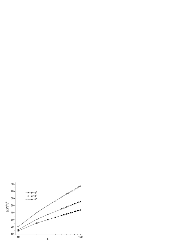
Figure 2: Demonstration of the logarithmic scaling law (16) of the CrMES extensions for the square Ising model, shown for the three levels of accuracy chosen. Note that the extensions $\Delta E^{\ast}$ are defined to be dimensionless as discussed in Section III.

Table 3 gives the estimates for the above amplitudes for sizes $L=10-50$, $L=10-100$ and $L=50-100$. Also Fig.2 shows the behavior of theses extensions versus lattice size. As was expected on physical grounds, the extensions of CrMES follow the same asymptotic law with the specific heat in the critical region and provide a new independent method of estimating critical behavior via the finite size scaling analysis. Since, $\Delta\widetilde{E}_{c}\cong\Delta\widetilde{E}^{\ast}-2$ for all lattice sizes, the extensions of the CrMES at the exact critical temperature follow the same scaling law. We end this section by noting that one can use the data in Table 1 to estimate from the law (2b) the critical exponent $\nu$ and the critical temperature $T_{c}$.

IV The Three - Dimensional Ising Model

Despite the intense effort made over the last decades, the three-dimensional Ising model has defied exact solution domb60 ; fishe67 and though it has been investigated extensively by various numerical methods, is still a matter of sophisticated numerical analysis nicke80 ; brezi74 ; guill80 ; guill87 ; pawle84 ; blote89 ; blote89b ; liu89 ; landa76 ; barbe85 ; paris85 ; hoogl85 ; bhano86 ; chen82 ; guttm94 ; koles94 ; nicke90 ; nicke91 ; adler83 ; talap96 ; blote95 ; blote96b ; deng03 ; blote97 ; hanse91 ; buter97 ; guida98 ; garci ; buter02 . The critical properties of the model, i.e., the critical temperature $T_{c}$, the thermal and magnetic scaling exponents $y_{t}$ and $y_{h}$, and also the leading thermal irrelevant exponent $y_{i}$ seem to be known with good accuracy deng03 . However, the absence of exact results creates, at least in principle, a motive for disagreements garci ; deng03 . For many years reliable estimates for $T_{c}$ and the critical exponents have been obtained by series-expansion data, $\varepsilon$-expansion studies, Monte Carlo renormalization group studies and the coherent anomaly method nicke80 ; brezi74 ; guill80 ; guill87 ; pawle84 ; blote89 ; blote89b ; liu89 ; chen82 ; guttm94 ; koles94 ; nicke90 ; nicke91 ; adler83 ; buter02 .

The traditional Monte Carlo sampling, importance sampling and histogram techniques, have been used also to investigate the three-dimensional Ising model ferre91 ; landa76 ; barbe85 ; paris85 ; hoogl85 ; bhano86 ; blote95 ; blote96b ; deng03 but only recently deng03 such studies have provided accurate estimates of the critical exponents. There are two reasons for the modest accuracy obtained in these Monte Carlo simulations. Firstly, extended runs are necessary to reduce the systematic and statistical errors, which arise due to the finite number of samples taken. Secondly, corrections to scaling are much more important in three than in two dimensions. The leading irrelevant thermal exponent for the three-dimensional Ising model has the value $y_{i}=-0.821(5)$ deng03 and this means that corrections decay relatively slowly. The two effects of finite sampling time and finite system size become intertwined and jeopardize the finite size scaling analysis. In particular, it has been very difficult to accurately estimate the thermal critical exponent from finite size scaling analysis of Monte Carlo specific-heat data close to the pseudo-critical temperatures.

Blote et al blote95 have presented an extensive Monte Carlo simultaneous analysis of three cubic Ising models belonging to the same universality class. Their data were obtained by several “cluster” algorithms and their analysis included a finite-size scaling study for the specific heat anomaly of the simple cubic Ising model (section $5.2$ in blote95 ). Furthermore, in a recent analogous study Deng and Blote deng03 proposed a different “better” route for the estimation of the thermal exponent. In this latter study, a quantity ($Q_{p}$) that correlates the magnetization distribution with the energy density deng03 , which has a stronger divergence with respect to the system-size, is used. In general, it appears that the traditional route for the estimation of the thermal critical exponent, via specific-heat data, has been overlooked over the years because of the problems faced in trying to fit these data. This is entirely understandable by comparing the high accuracy obtained in the recent paper by Y. Deng and H. Blote deng03 ($y_{t}=1.5868(3)$), with the modest estimate ($y_{t}=1.60(2)$) in Blote et al blote95 . In view of this situation, it is of interest to apply our proposal for estimation of the DOS via a Wang-Landau random walk in the CrMES and study again the so produced numerical data for the specific-heat peaks. Furthermore, it is most appealing to examine whether the data for the r-dependent extensions of the CrMES, give when subjected to finite-size analysis, estimates in agreement with the already known values of the thermal critical exponent.

We may, following Blote et al blote95 , use an expansion for the specific-heat values close to the critical point of the form:

$$C_{L}=L^{2y_{t}-d}\left(q_{o}+q_{1}(K-K_{c})L^{y_{t}}\right)+p_{o}+rL^{2y_{t}-d+y_{i}}+s_{o}L^{y_{t}-d}$$ (17)

In this expansion the renormalization group behavior of the free energy with a scale factor ($l$) has been used. Moreover, the existence of an irrelevant field has been assumed and some terms from the more general expansion have been omitted as dominated by the correction terms included in (17) (see equation $(21)$ and discussion in blote95 ). Blote et al blote95 used a fixed value for the irrelevant exponent: $y_{i}=-0.83$ and the value $K_{c}=0.2216547$ ($K=\frac{J}{K_{B}T}$) for the critical temperature. Thus, in order to estimate the thermal critical exponent $y_{t}$, five more parameters ($q_{o},q_{1},p_{o},\textit{r},s_{o}$) are involved in (17). This “many-parametric” fit gave the estimate $y_{t}=1.60(2)$, but the errors reported of all five parameters were very large (up to 100%) even for the coefficients $q_{o}$($q_{1}$) of the leading singularity.

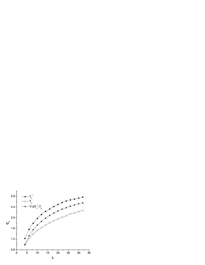
Figure 3: Specific heat values (in units of $k_{B}$) of the cubic Ising model for the three temperatures mentioned in the text.

We applied the CrMES Wang-Landau scheme to obtain the DOS for lattice sizes $L=4-32$ for the simple cubic Ising lattice. For each lattice, several random walks on the selected restricted energy space were performed for averaging. The numbers of these walks varied with the lattice size, ranging from $30$ walks for the size $L=4$ to $100$ walks for the size $L=32$. We used the same procedures for averaging and estimating the errors, described in the previous section. In this way we obtained data for the specific heat in the critical region following the method described in Section II. We also attempted a similar analysis, based on the expansion (17), fixing the irrelevant exponent to the value $y_{i}=-0.821$ from Y. Deng and H. Blote deng03 . In particular, we concentrated on three temperatures: the “pseudo-critical” temperatures $T_{L}^{\ast}$, a “good” approximation $T_{c}^{\prime}=4.51152..$ ($K_{c}=0.2216547$ blote95 ) for the exact critical temperature $T_{c}$, and finally a “lower” temperature defined for each lattice by $\widehat{T}_{L}=2T_{L}^{\ast}-T_{c}^{\prime}$. Fig.3 shows the values of the specific heat at these temperatures as function of the lattice size. In Table 4 we present our estimates for the pseudo-critical temperatures $T_{L}^{\ast}$, the corresponding values of the specific heat $C_{L}^{\ast}$ and the extensions of the critical minimum energy subspaces (CrMES) $\Delta\widetilde{E}^{\ast}(\textit{r})$ for the three levels of accuracy $\textit{r}=10^{-3},10^{-4},10^{-6}$. From Fig.3 one can observe a rather smooth behavior with relatively small errors. The estimates for the lower temperature $\widehat{T}_{L}$ seem to be the most accurate. However, our attempt to fit these data in the expansion (17) produced modest estimates for the thermal exponent and very large errors for almost all other parameters. We found estimates of the same order with those given in Blote et al blote95 , at least for the dominant terms of the expansion, but such fittings are not reliable since the errors in all coefficients are very large.

In order to suppress the errors we tried to omit further terms from the expansion and we searched for stable forms as we disregarded the smaller lattice sizes from the fittings. Thus, we have observed the fittings, for several alternative truncations of the expansion, in the following six successive intervals: $L=4-32,6-32,...,14-32$. Among other possibilities, we kept (as non-zero) only the correction terms with coefficients $q_{o}$ and r in (17). The resulting estimates for the thermal exponent shifts to lower values as we move to larger-size intervals. Thus, although some of the estimates seem to be very close to the expected value of the critical thermal exponent, the overall behavior is rather unsettled producing estimates for $y_{t}$ in a rather wide range: $1.56-1.62$. An explanation for this behavior may be the following: as we move to larger lattice sizes the relative contribution of the various correction terms is changing and this make the analysis for these relatively small sizes very sensitive. However, some quite acceptable exceptions will be now mentioned: Consider, the specific heat values at the temperature $T_{c}^{\prime}=4.51152..$ and fix the value of the constant contribution in the neighborhood of $p_{o}\cong-1.5$, then allow $q_{o}$ and r to vary and make successive fittings for all intervals from $L=4-32$ up to $L=14-32$. These six fittings are very good and stable and produce estimates with very small errors. They give approximately the same value for the thermal exponent but also for the coefficients $q_{o}$ and r. This is true for even larger-size ranges but with larger errors. Considering the mean and the standard deviation of these six estimates (see Appendix) we find:

$$y_{t}=1.5878(31),\;\ q_{o}=2.08(6),\;\ \textit{r}=-0.43(20)$$ (18)

The above values should be compared with the values given in Blote et al blote95 . Our error limits are about $10$ times smaller and our estimate for the thermal exponent is very close to the value given by Y. Deng and H. Blote deng03 ($y_{t}=1.5868(3)$). The constant term and the main amplitude $q_{o}$ are just marginally in agreement with the values in Blote et al blote95 ($p_{o}=-0.8(7)$ and $q_{o}=1.5(5)$). This is a good coincidence and we may speculate that this exceptional case is very close to the exact result. Its appearance may be well related to the absence of the term with coefficient $q_{1}$ in the expansion, which for the other two temperatures may cause fitting problems. Furthermore, a stable sequence of fittings using the specific heat values at the lower temperature $\widehat{T}_{L}=2T^{\ast}_{L}-T^{\prime}_{c}$ is also given in Appendix. This sequence produces estimates for the thermal exponent $y_{t}$, comparable with that given in (18). Finally, note that we may use the values for $T^{\ast}_{L}$ to estimate the critical temperature $T_{c}$ and/or the critical exponent $\nu$ from (2b). The fitting for the case $L=12-32$ provides good values for both these critical parameters, without even using correction terms. To obtain values comparable in accuracy, with the best known estimates, a study of several different thermodynamic quantities may be necessary (see for instance ferre91 ).

Let us now examine the verification of our proposal for the scaling of the extensions of the CrMES. The estimates for these extensions are included in Table IV. Once again one can observe that the reported relative errors for these extensions (for the three levels of accuracy) are significantly smaller (by a factor of $10$) than those concerning the values of the specific heat. It is also remarkable that for sizes up to $L=16$ there are no errors at all for these extensions. Note that, even the restriction of the energy space using the larger value of the accuracy level (r) will not introduce errors in the specific heat, larger than those generated from the Wang-Landau random walk. Thus, if we minimize our requirements so that we only calculate the value of the specific heat at the pseudo-critical temperature, then the energy subspace needed is only $1/20$ of the total energy space for the $32\times 32\times 32$ cubic lattice. The extended energy ranges used for the estimation of the parameters in Table 4 and the values of the specific heat at the temperatures $T_{c}^{\prime}$, $T^{\ast}_{L}$ are summarized in the Appendix (see Table 6).

When the extensions of the CrMES are subjected to a finite size analysis using a many-parametric expansion as (17), we again find modest estimates for the thermal exponents and large errors in all other parameters. However, we have discovered that the dominant contributions now correspond to the terms with coefficients $q_{o}$ and r in (17). Introducing a more convenient notation we assume that these extension scale as:

$$\Psi(r)\equiv\left(\frac{\Delta\widetilde{E}^{\ast}_{r}}{L^{d/2}}\right)^{2}\simeq q(r)L^{2y_{t}-d}+p(r)L^{2y_{t}-d+y_{i}}$$ (19)

Table 5 shows successive fits on the above form for the three levels of accuracy. As previously the value of the irrelevant exponent is fixed to the value $y_{i}=-0.821$, but no other parameter is fixed. The last two fittings give close agreement (almost to the third decimal place) with the best known estimate of the thermal critical exponent deng03 . There is a small shift of the estimated thermal critical exponent to a lower value as we move to larger lattice sizes indicating possible existence of further correction terms. This shift is similar, but considerably smaller, with the one detected in our fittings for the specific heat values at the pseudo-critical temperatures. Thus, we can conclude that the proposed scaling law of the CrMES introduced in this paper is correct and can be considered as a new effective technique for estimating the thermal critical exponent.

V Conclusions

We have presented a simple and efficient approximation scheme, which greatly facilitates the application of Wang-Landau sampling in large systems for the estimation of critical behavior. In particular, we have applied our proposal to study the finite size behavior of the specific heat for both square and cubic Ising lattices. It has been shown that one needs only a relatively small part of spectral degeneracies in order to obtain good estimation of the specific-heat peaks. We have described the outline of an algorithm for identifying this part of the total energy range. Furthermore, a scaling law for the finite size behavior of the extensions of the critical part of the minimum energy subspace (CrMES) determined with the help of a predefined level of accuracy was proposed. This scaling law has been verified for both models studied in this paper and estimates of the thermal critical exponent for the three-dimensional case were obtained through this route. Also in the two-dimensional case the expected logarithmic behavior was confirmed.

In this paper we have considered an important aspect of the problem concerning the extraction of the critical behavior, by employing finite-size scaling theory and the recent methods that directly calculate the density of states of classical statistical models. Future applications of the proposed scheme concern several models, for which we may use the Wang-Landau technique or the broad histogram ferre98 ; lima00 and transition matrix wang02 ; wang99 methods. However, the main goal is to improve accuracy and obtain high-quality data for substantially larger lattices. This may be achieved now with the help of our proposal but the need of a comprehensive examination of all “systematic” and statistical errors of the DOS methods is now indispensable. The errors, for example, when implementing the Wang-Landau method are coming from several sources. There are errors coming from the finite accuracy of the histogram flatness which may propagate and amplify through the process of connecting the energy ranges in a multi-range approach. There are also errors stemming from the incomplete detailed balance condition. As always, we may expect errors from the random number generation and the usual statistical fluctuations. An “optimization” of all these errors, seems to be at this time quite demanding. The multi-range approach described in Section II, that leaves unchanged the central subinterval degeneracies, is only one “ingredient” of such an optimization.

VI Appendix

Here we present specific heat values obtained by the proposed CrMES Wang-Landau method and give further details of the fitting attempts to the expansion (17) for the cubic Ising model. Table 6 gives the specific heat values and specifies the extended energy subspace (CrMES) used in this paper in order to obtain the accuracy level $r=10^{-6}$ and also estimate the extensions given in Table 4. The values $C(T_{c}^{\prime})$ of the third column of Table 6 are now fitted in the following scaling formula:

$$C(T_{c}^{\prime})=-1.5+q_{o}L^{2y_{t}-3}+rL^{2y_{t}-3.821}$$ (20)

The successive estimates for the amplitudes $q_{o}$ and $r$ and the thermal exponent $y_{t}$ are given in Table 7. Their mean values over the fitting ranges appear in our proposal in (18). Finally the values of $C(\widehat{T}_{L})$ are fitted in a more restricted form (21), given below. The produced estimates are shown in Table 8.

$$C(\widehat{T}_{L})=-0.3+q_{o}L^{2y_{t}-3}-2L^{2y_{t}-3.821}$$ (21)

The particular values of the expansion (17) for $p_{o}$ and $p_{o}$ and $r$ chosen in (20) and (21) respectively, provide a stable and convincing picture for the estimation of the thermal exponent.

Table 1: Exact and approximate Wang-Landau (WL) results for the square Ising model. “Pseudo-critical” temperatures $T^{\ast}_{L}$, corresponding specific heat values $C^{\ast}_{L}$ and specific heat values at the exact critical temperatures $C_{L}(T_{c})$. The exact DOS has been obtained by the algorithm provided in beale96 .

$L$	$T^{*}_{L}$: exact	$T^{*}_{L}$: WL	$C^{*}_{L}$: exact	$C^{*}_{L}$: WL	$C_{L}(T_{c})$: exact	$C_{L}(T_{c})$: WL
10	2.34459		1.30906		1.26002
14	2.32407		1.48356		1.43117
20	2.30820		1.66628		1.61116
24	2.30190		1.75899		1.70273
30	2.29553		1.87193		1.81450
34	2.29251		1.93507		1.87706
40	2.28909		2.01686		1.95818
44	2.28731		2.06473		2.00570
50	2.28518	2.2853(3)	2.12885	2.1338(150)	2.06938	2.0791(150)
54		2.2835(3)		2.1690(200)		2.1150(250)
60		2.2825(3)		2.2275(300)		2.1620(350)
64		2.2816(3)		2.2523(350)		2.1860(300)
70		2.2809(3)		2.2910(350)		2.2242(350)
74		2.2805(4)		2.3240(400)		2.2587(400)
80		2.2796(4)		2.3630(400)		2.3000(450)
84		2.2792(4)		2.3900(450)		2.3240(500)
90		2.2781(4)		2.4200(450)		2.3650(500)
94		2.2779(4)		2.4460(500)		2.3840(500)
100		2.2775(4)		2.4710(600)		2.4120(500)

Table 2: Critical Minimum Energy Subspace (CrMES) extensions for the square Ising model calculated for the three predefined levels of accuracy r. Note that the relative errors for these extensions are much smaller than those for the corresponding specific heats.

$L$	exact	WL	exact	WL	exact	WL	exact	WL	exact	WL	exact	WL
	$\Delta\widetilde{E}^{*}(r_{1})$	$\Delta\widetilde{E}^{*}(r_{1})$	$\Delta\widetilde{E}^{*}(r_{2})$	$\Delta\widetilde{E}^{*}(r_{2})$	$\Delta\widetilde{E}^{*}(r_{3})$	$\Delta\widetilde{E}^{*}(r_{3})$	$\Delta\widetilde{E}_{c}(r_{1})$	$\Delta\widetilde{E}_{c}(r_{1})$	$\Delta\widetilde{E}_{c}(r_{2})$	$\Delta\widetilde{E}_{c}(r_{2})$	$\Delta\widetilde{E}_{c}(r_{3})$	$\Delta\widetilde{E}_{c}(r_{3})$
10	38		40		45		36		39		43
14	63		68		74		62		66		72
20	101		111		127		99		109		126
24	126		140		161		124		138		159
30	165		184		213		163		182		211
34	191		213		248		190		211		246
40	232		259		302		230		257		300
44	259		290		339		257		288		336
50	301	301	337	337	394	394	299	299	335	335	392	392
54		329		368		432		327		366		429
60		371		416		489		369		414		486
64		400		448		527		398		446		524
70		442(1)		497		584(1)		440(1)		494(1)		582
74		472(1)		530(1)		624(1)		470(1)		528(1)		621(1)
80		516(1)		580(2)		682(2)		514(1)		577(1)		679(2)
84		545(1)		613(2)		722(2)		543(1)		610(2)		719(2)
90		589(1)		663(2)		781(2)		587(1)		660(2)		778(2)
94		619(2)		696(2)		821(2)		616(2)		693(2)		818(2)
100		662(2)		745(2)		881(2)		659(2)		742(2)		877(2)

Table 3: Estimates of amplitudes obtained by fitting (16) to the CrMES extensions presented in Table 2 for the square Ising model.

$L$		$A(r)$	$B_{1}(r)$
	$\Psi(r_{1})$	10.08(8)	-34(2)
$10-50$	$\Psi_{(}r_{2})$	12.81(11)	-55(3)
	$\Psi(r_{3})$	17.81(16)	-92(4)
	$\Psi(r_{1})$	9.90(3)	-32(1)
$10-100$	$\Psi(r_{2})$	12.65(4)	-52(1)
	$\Psi(r_{3})$	17.75(5)	-92(2)
	$\Psi(r_{1})$	9.83(3)	-29(2)
$50-100$	$\Psi(r_{2})$	12.60(4)	-51(2)
	$\Psi(r_{3})$	17.81(3)	-96(2)

Table 4: Estimates obtained via Wang-Landau CrMES scheme described in this paper for the cubic Ising model.“ Pseudo-critical” temperatures $T^{*}_{L}$, corresponding specific heat values and CrMES extensions for the three levels of accuracy $r$.

$L$	$T^{*}_{L}$	$C(T^{*}_{L})$	$\Delta\widetilde{E}^{*}(r_{1})$	$\Delta\widetilde{E}^{*}(r_{2})$	$\Delta\widetilde{E}^{*}(r_{3})$
4	4.1150(20)	1.2242(30)	45	47	51
6	4.2752(20)	1.5632(50)	122	133	148
8	4.3495(20)	1.7920(70)	215	236	269
10	4.3944(20)	1.9720(100)	325	359	413
12	4.4210(20)	2.1180(170)	453	502	579
14	4.4395(30)	2.2365(240)	596	661	766
16	4.4532(30)	2.3243(380)	753	836	971
18	4.4623(30)	2.4177(390)	925(1)	1029(2)	1195(2)
20	4.4702(30)	2.4955(400)	1106(1)	1232(2)	1433(2)
22	4.4758(30)	2.5670(420)	1302(2)	1451(2)	1690(2)
24	4.4796(30)	2.6242(450)	1504(6)	1677(6)	1954(10)
26	4.4854(35)	2.6648(750)	1722(8)	1926(8)	2244(10)
28	4.4879(45)	2.6966(800)	1951(8)	2178(8)	2544(10)
30	4.4911(45)	2.7325(900)	2178(10)	2432(10)	2845(10)
32	4.4929(50)	2.7688(900)	2430(10)	2716(10)	3176(12)

Table 5: Fitting attempts using (19) to estimate the thermal exponent $y_{t}$ from the CrMES extensions shown in Table 4 for the cubic Ising model. Note that the mean values (given in the footnote below) for $y_{t}$ are close to the value $y_{t}=1.5878(31)$ given in our proposal (18) and to the value $y_{t}=1.5868(3)$ of deng03 .

$L$		$q(r)$	$p(r)$	$y_{t}$
	$\Psi(r_{1})$	108(2)	-261(7)	1.596(3)
$4-32$	$\Psi_{(}r_{2})$	132(3)	-328(10)	1.601(3)
	$\Psi(r_{3})$	170(3)	-440(11)	1.610(3)
	$\Psi(r_{1})$	107(4)	-255(14)	1.598(5)
$6-32$	$\Psi(r_{2})$	130(5)	-321(19)	1.602(5)
	$\Psi(r_{3})$	179(5)	-476(18)	1.603(3)
	$\Psi(r_{1})$	115(5)	-293(20)	1.588(5)
$8-32$	$\Psi(r_{2})$	142(6)	-373(27)	1.591(6)
	$\Psi(r_{3})$	189(6)	-524(27)	1.596(4)
	$\Psi(r_{1})$	129(6)	-356(25)	1.574(6)
$10-32$	$\Psi(r_{2})$	155(9)	-439(40)	1.579(7)
	$\Psi(r_{3})$	203(8)	-589(39)	1.587(6)

Table 6: Specific heat values for the cubic Ising model at the two temperatures $\widehat{T}_{L}$ and $T_{c}^{\prime}$ defined in the text (see also footnote). The counting variables $ie(E^{\prime}_{min})$ and $ie(E^{\prime}_{max})$, where $ie(E)=(E+3N)/4+1$, specify the extended range used in this work. The portion of the energy space used in our calculations is given in the last column.

$L$	$C(\widehat{T}_{L})$	$C(T_{c}^{\prime})$	$ie(E^{\prime}_{min})$	$ie(E^{\prime}_{max})$	$(E^{\prime}_{max}-E^{\prime}_{min})/(E_{max}-E_{min})$
4	0.9954(20)	0.9776(20)	1	70	0.73
6	1.3230(30)	1.2256(30)	1	170	0.52
8	1.5471(60)	1.3908(60)	30	380	0.46
10	1.7245(80)	1.5248(80)	150	670	0.35
12	1.8610(80)	1.6300(80)	360	1100	0.29
14	1.9846(150)	1.7234(150)	710	1670	0.23
16	2.0854(250)	1.8129(250)	1220	2410	0.19
18	2.1790(350)	1.8883(350)	1800	3500	0.19
20	2.2527(380)	1.9555(380)	2800	4520	0.14
22	2.3190(380)	2.0170(380)	3900	5960	0.13
24	2.3728(400)	2.0720(400)	5250	7650	0.12
26	2.4307(470)	2.1458(470)	6870	9680	0.11
28	2.4738(500)	2.1772(600)	8790	11970	0.10
30	2.5209(650)	2.2345(800)	11150	14590	0.09
32	2.5515(700)	2.2700(850)	13700	17650	0.08

Table 7: Successive fittings for the specific heat values $C(T_{c}^{\prime})$. Scaling expansion (20) is used.

$L$	$q_{o}$	$r$	$y_{t}$
4-32	2.09(2)	-0.46(6)	1.5869(2)
6-32	2.04(4)	-0.27(10)	1.5902(22)
8-32	2.03(6)	-0.27(17)	1.5904(33)
10-32	2.03(9)	-0.27(28)	1.5904(50)
12-32	2.11(13)	-0.54(45)	1.5860(71)
14-32	2.17(2)	-0.76(74)	1.5828(105)

Table 8: Successive fittings for the specific heat values $C(\widehat{T}_{L})$. The expansion used is given in (21).

$L$	$q_{o}$	$y_{t}$
4-32	1.633(7)	1.592(1)
6-32	1.625(9)	1.593(1)
8-32	1.627(11)	1.593(1)
10-32	1.637(13)	1.592(1)
12-32	1.650(15)	1.590(1)
14-32	1.671(15)	1.588(2)
16-32	1.692(16)	1.586(2)
18-32	1.718(14)	1.584(1)
20-32	1.733(17)	1.582(2)

References

- (1) N. Metropolis, A. W. Rosenbluth, M. N. Rosenbluth, A. H. Teller and E. Teller, J. Chem. Phys. 21, 1087, (1953).
- (2) R. J. Glauber, J. Math. Phys. 4, 294, (1963).
- (3) A. B. Bortz, M. H. Kalos and J. L. Lebowitz, J. Comput. Phys. 17, 10, (1975).
- (4) K. Binder, Rep.Prog. Phys. 60, 487, (1977).
- (5) M. E. J. Newman and G. T. Barkema, Monte Carlo Methods in Statistical Physics, Clarendon Press, Oxford, (1999).
- (6) D. P. Landau and K. Binder, A Guide to Monte Carlo Simulations in Statistical Physics, Cambridge University Press, (2000).
- (7) J.Lee, Phys. Rev. Lett. 71, 211, (1993).
- (8) B. A. Berg and T. Neuhaus, Phys. Rev. Lett. 68, 9, (1992).
- (9) A. M. Ferrenberg and R. H. Swendsen, Phys. Rev. Lett. 61, 2635, (1998).
- (10) A. R. Lima, P. M. C. de Oliveira, and T. J. P. Penna, J. Stat. Phys. 99, Nos.3/4, (2000).
- (11) J. -S. Wang and R. H. Swendsen, J. Stat. Phys. 106, Nos. 1/2, (2002).
- (12) J. -S. Wang, T. K. Tay and R. H. Swendsen, Phys. Rev. Lett. 82, 476, (1999).
- (13) F. Wang and D. P. Landau, Phys. Rev. Let. 86, 2050, (2001).
- (14) F. Wang, D. P. Landau, Phys. Rev. E 64, 056101, (2001).
- (15) B. J. Schulz, K. Binder and M. Muller, Int. J. Mod. Phys. C 13, 477, (2001).
- (16) B. J. Schulz, K. Binder, M. Muller and D. P. Landau, Phys. Rev. E 67, 067102, (2003).
- (17) D. P. Landau and F. Wang, Comput. Phys. Comm. 147, 674, (2002).
- (18) A. E. Ferdinand and M. E. Fisher, Phys. Rev. 185, 832, (1969).
- (19) M. E. Fisher, Critical Phenomena, ed. M. S. Green, Academic Press, London, (1971).
- (20) V. Privman, Finite Size Scaling and Numerical Simulation of Statistical Systems, World Scientific, Singapore, (1990).
- (21) K. Binder, Computational Methods in Field Theory, eds. C. B. Lang and H Gausterer, Springer, Berlin, (1992).
- (22) P. de Beale, Phys. Rev. Lett. 76, 1, (1996).
- (23) A. M. Ferrenberg and D. P.Landau, Phys.Rev. B 44, 10, (1991).
- (24) M. E. Fisher, Rep. Prog. Phys. 30, 615, (1967).
- (25) C. Domb, Adv. Phys. 9, 149, (1960).
- (26) B. G. Nickel, Phase Transitions: Cargese 1980 (Plenum, New York, 1982), 291.
- (27) E. Brezin, J. -C. Le Guillou and J. Zinn-Justin, Phys. Lett. 47A, 285, (1974).
- (28) J. -C. Le Guillou and J. Zinn-Justin, Phys. Rev. B 21, 3976, (1980).
- (29) J. -C. Le Guillou and J. Zinn-Justin, J. Phys. (Paris) 48, 19, (1987).
- (30) G. S. Pawley, R. H. Swendsen, D. J. Wallace and K. G. Wilson Phys. Rev. B 29, 4030, (1984).
- (31) H. W. J. Blote, J. de Bruin, A. Compagner, J. H. Crookewit, Y. T. J. C. Fonk, J. R. Heringa, A. Hoogland, and A. L. van Willigen Europhys. Lett. 10, 105, (1989).
- (32) H. W. J. Blote, A. Compagner, J. H. Crookewit, Y. T. J. C. Fonk, J. R. Heringa, A. Hoogland, T. S. Smit, and A. L. van Willigen, Physica A 161, 1, (1989).
- (33) A. J. Liu and M. E. Fisher, Physica A 165, 35, (1989).
- (34) D. P. Landau, Phys. Rev. B 14, 255, (1976).
- (35) M. N. Barber, R. B. Pearson, D. Toussaint, and J. L. Richardson, Phys. Rev. B 32, 1970, (1985).
- (36) G. Parisi and F. Rapuano, Phys. Lett. 157B, 301, (1985).
- (37) A. Hoogland, A. Compagner, and H. W. J. Blote, Physica A 132, 593, (1985).
- (38) G. Bhanot, D. Duke, and R. Salvador, Phys. Rev. B 33, 7841, (1986).
- (39) J. H. Chen, M. E. Fisher and B. G. Nickel, Phys. Rev. Lett. 48, 630, (1982).
- (40) A. J. Guttmann and I. G. Enting, J. Phys. A 27, 8007, (1994).
- (41) M. Kolesik and M. Suzuki, Pysica A 27, 8007, (1994).
- (42) B. G. Nickel and J. J. Rehr, J. Stat. Phys. 61, 1, (1990).
- (43) B. G. Nickel, Physica A 177, 189, (1991).
- (44) J. Adler, J. Phys. A 16, 3585, (1983).
- (45) A. L. Talapov and H. W. J. Blote, J. Phys. A 29, 5727, (1996).
- (46) H. W. J. Blote, E. Luijten, and J. R. Heringa, J. Phys. A 28, 6289, (1995).
- (47) H. W. J. Blote, J. R. Heringa, A. Hoogland, E. W. Meyer and T. S. Smit, Phys. Rev. Lett. 76, 2613, (1996).
- (48) Y. Deng and H. W. J. Blote, Phys. Rev. E 68, 036125, (2003).
- (49) H. W. J. Blote, L. N. Shchur, and A. L. Talapov, Int. J. Mod. Phys. C 10, 1137, (1997).
- (50) M. Hansebusch, K. Pinn, and S. Vinti, Phys. Rev. B 59, 11471, (1991).
- (51) P. Butera and M. Comi, Phys. Rev. B 56, 8212, (1997).
- (52) R. Guida and J. Zinn-Justin, J. Phys. A 31, 8103, (1998).
- (53) J. Garcia, J. A. Gonzalo and M. I. Marques, e-print cond-mat/0211270.
- (54) P. Butera and M. Comi, Phys. Rev. B 65, 144431, (2002).