Non-order parameter Langevin equation for a bounded Kardar-Parisi-Zhang universality class

Abstract

We introduce a Langevin equation describing the pinning-depinning phase transition experienced by Kardar-Parisi-Zhang interfaces in the presence of a bounding “lower-wall”. This provides a continuous description for this universality class, complementary to the different and already well documented one for the case of an “upper-wall”. The Langevin equation is written in terms of a field that is not an order-parameter, in contrast to standard approaches, and is studied both by employing a systematic mean-field approximation and by means of a recently introduced efficient integration scheme. Our findings are in good agreement with known results from microscopic models in this class, while the numerical precision is improved. This Langevin equation constitutes a sound starting point for further analytical calculations, beyond mean-field, needed to shed more light on this poorly understood universality class.

today

1 Introduction

It was shown a few years ago that the introduction of a limiting or bounding wall into a Kardar-Parisi-Zhang (KPZ) interface model [1, 2] leads to quite different phenomenologies depending on whether the wall is an “upper” or a “lower” one [3, 4, 5, 6]. This result, the origin of which can be traced back to the absence of height-inversion symmetry in KPZ interfacial dynamics [3, 6], has been verified for several discrete interfacial KPZ-like models [3, 6, 7]. In any of these cases, once a limiting wall is introduced, there are two different phases: a depinned one in which the KPZ-interface moves freely away from the wall, and a pinned one, with a finite stationary average distance from the wall. Separating these two phases there is a nonequilibrium phase transition, whose criticality encompasses also that of synchronizing extended systems [8, 9], nonequilibrium wetting phenomena [10, 11, 12], transitions occurring in DNA alignment problems [3, 6], phenomena related to Burgers’ turbulence [3], bounded directed-polymers in random-media [3], etc. Characterizing and distinguishing between the two above-mentioned pinning-depinning universality classes, with an upper or a lower wall respectively, is therefore a relevant task in many different contexts, as well as a chief theoretical problem.

In terms of Langevin equations, an ideal framework to discuss universality issues, KPZ-like interfaces are described by the celebrated and profusely studied KPZ equation [1]:

$${\partial{h(r,t)}\over{\partial{t}}}=a+\lambda(\nabla h(r,t))^{2}+D\nabla^{2}h(r,t)+\sigma\eta(r,t),$$ (1)

where $h(r,t)$ is the interface height at position $r$ and time $t$, $\lambda$, D, and $\sigma$ are constants, and $\eta$ is a Gaussian white noise. In what follows, and without loss of generality, we take $\lambda=+D$. Alternatively, we could also have fixed a given type of limiting wall, for instance, a lower, rigid substrate on top of which the interface grows, and observe the two different classes of depinning transitions under scrutiny depending on the sign of $\lambda$ [13].

Let us consider now equation (1) in the presence of an exponential, upper wall, i.e. including the additional term $-b\exp(q\ h)$, with $b>0$ and $q>0$. A transition takes place from a regime characterized by depinned interfaces, flowing to minus infinity for sufficiently negative values of $a$, to one with interfaces pinned to the wall, with exponentially cutoff positive values of $h$, above a certain threshold $a_{c}$. This can also be visualized by performing a Cole-Hopf transformation, $n=\exp(h)$ [14], which leads to,

$${\partial{n(r,t)}\over{\partial{t}}}=D\nabla^{2}n(r,t)+an(r,t)-bn(r,t)^{1+q}+\sigma n(r,t)\eta(r,t).$$ (2)

This is a multiplicative noise equation (interpreted in the Stratonovich sense [15, 16]) defining a, well established by now, phase transition with a corresponding set of critical exponents that characterizes the so-called multiplicative noise 1 (MN1) universality class [4, 5, 6, 17]. At the transition point and in the depinned phase the stationary average value of the order-parameter, $\bar{n}$, is zero, while it is non-vanishing above the transition point. The critical exponents and other universal features in this class are not affected by the value of $q$, i.e. by the “impenetrability degree” of the wall; indeed, in microscopic models the wall is typically a hard substrate, corresponding to $q\rightarrow\infty$.

On the other hand, by introducing in equation (1) a lower wall, $b\exp(-qh)$, hindering the interface height to take negative values, depinned interfaces flow towards plus infinity. In this case, a natural order-parameter, equivalent to that for the upper-wall class, going to zero at the transition point, is $m=\exp(-h)$, and the corresponding depinning transition is in the so-called multiplicative noise 2 (MN2) universality class [6, 3, 7, 18, 12].

Consequently, we perform the change of variables $m=\exp(-h)$ to obtain [7, 19]:

$${\partial{m(r,t)}\over{\partial{t}}}=D\nabla^{2}m-2D{(\nabla m)^{2}\over m}-am-bm^{1-q}+\sigma m\eta(r,t),$$ (3)

where some space and time dependencies have been omitted to simplify the notation. Observe that owing to the $(\nabla m)^{2}/m$ term the equation becomes singular above the transition point, where $\bar{m}=0$. Equation (3) was studied in detail, both numerically and using mean-field approaches, in [7], but no sound result could be obtained owing to the presence of the singular gradient term. Therefore, all the known results for this universality class come from numerical [7, 12] as well as some analytical (mean-field like) [18] studies of discrete microscopic models. Let us also stress that direct numerical integrations of KPZ-like Langevin equations (before applying the Cole-Hopf transformation) are uncontrollable due to well-documented numerical instabilities [20].

Aimed at filling the gap between discrete and continuous levels of description for the MN2 universality class, in this article we show that the MN2 phenomenology can be captured by an alternative, multiplicative-noise, Langevin equation. To that purpose, we take the KPZ equation in the presence of a lower-wall and perform the change of variables, $n=\exp(h)$, leading to

$${\partial{n(r,t)}\over{\partial{t}}}=D\nabla^{2}n+an+bn^{1-q}+\sigma n\eta(r,t),$$ (4)

which takes a particularly simple form for $q=1$ although, as in the MN1 class, the precise value of $q>0$ is not expected to affect universal features. Note the remarkable difference between equations (2) and (4): while in the former $n$ is an order-parameter for the MN1 transition, in equation (4) for the MN2 class, it is not, as it diverges at the transition point and in the depinned phase. Therefore equation (4) is not an order-parameter Langevin equation and it is $m=1/n$ that is to be monitored once the equation for $n$ is integrated. Typically, Langevin equations are written in terms of a vanishing-at-the-transition order-parameter so that series expansions, truncation of power-series to lowest orders can be employed and the applicability of standard perturbative techniques is viable. This is in contrast with equation (4). Furthermore, the noise amplitude diverges at the transition point. This apparent ill-behavior may be the reason why equation (4) has been ignored so far in the literature.

In what follows we study the non-order parameter Langevin equation for the MN2 class, equation (4), using standard mean-field approaches and integrating it numerically. Despite of the presence of apparent pathologies and divergences at (and above) the transition point, we find that equation (4) reproduces the previously known results for this universality class. In passing, we improve the numerical precision of the corresponding critical exponents. This constitutes a step forward in the general understanding of nonequilibrium phase transitions into absorbing states, allows for a better comparison with the MN1 class, gives a new starting point for future analytical approaches, and serves as an example of a phase transition best characterized in terms of an equation for a diverging field that is not an order-parameter.

2 Mean-Field analysis

Standard mean-field approaches usually neglect spatial and noise-induced fluctuations. For Langevin equations characterizing spatially extended systems with multiplicative noise, however, this approximation has proved to be too crude and unreliable in any dimension [17] as both spatial structure and noise are relevant features. Therefore, more elaborated methods are required to obtain a sound qualitative picture of the transition [21, 22, 23]. A mean-field approach tailored to account properly for the noise term and the spatially-varying order-parameter consists in discretizing the Laplacian term as $1/2d\sum_{j}(n_{j}-n_{i})$, where $d$ is the system dimensionality and the sum is over the nearest-neighbors of site $i$ [22, 23]. When these latter are substituted by their average value $\bar{n}$, a closed Fokker-Planck equation (which involves no approximation in the noise) is obtained for $P(n,\bar{n})$. The stationary solution of such an equation is found by imposing the self-consistency requirement [23]

$$\bar{n}={\int_{0}^{\infty}dn\ n\ P(n,\bar{n})\over\int_{0}^{\infty}dn\ P(n,\bar{n})}.$$ (5)

Note that this approach preserves the crucial role played by the multiplicative noise and includes the spatial coupling even if in an approximate (self-consistent) way. A detailed discussion of the results obtained with this method for the MN1 class can be found in [21]. Applying this procedure to equation (4) one readily obtains

$$P(n,\bar{n})\propto n^{{2(a-D)\over\sigma^{2}}-1}\exp\bigg{\{}-{2b\over\sigma^{2}qn^{q}}-{2D\bar{n}\over\sigma^{2}n}\bigg{\}},$$ (6)

and after defining $I_{p}(\bar{n})\equiv\int dn\ n^{p}\ P(n,\bar{n})$,

$$\bar{n}={I_{1}(\bar{n})\over I_{0}(\bar{n})},\qquad{\bar{m}}={I_{-1}(\bar{n})\over I_{0}(\bar{n})}.$$ (7)

To evaluate the scaling behavior of $I_{p}$ near the transition, when $\bar{n}$ becomes large, we first do the substitution $z=2D\bar{n}/\sigma^{2}n$ and then expand the newly generated term $\exp\{-2b/(\sigma^{2(1-q)}q)\times(z/2D\bar{n})^{q}\}$ to first order to obtain

$$I_{p}(\bar{n})\approx A_{p}\bar{n}^{p+\gamma}+B_{p}\bar{n}^{p+\gamma-q},$$ (8)

where $\gamma=2(a-D)/\sigma^{2}$ and $A_{p}$, $B_{p}$ are expressed using the Gamma function as

$$A_{p} = {\left(2D\over\sigma^{2}\right)}^{\gamma+p}\Gamma(-p-\gamma),$$

$$B_{p} = -{\left(2D\over\sigma^{2}\right)}^{p+\gamma-q}{2b\over\sigma^{2}q}\Gamma(-p-\gamma+q).$$ (9)

A direct calculation then yields $\bar{n}\sim{|a+\sigma^{2}/2|}^{-1/q}$ and ${\bar{m}}\sim|a+\sigma^{2}/2|^{1/q}$. Therefore, the order-parameter critical exponent is $\beta=1/q$ [24].

It is instructive to compare these results with those obtained using the same technique for equation (2), $\beta=\max\left(1/q,\sigma^{2}/(2D)\right)$ [22, 21]. That is, in the MN1 case two possible values of $\beta$, reminiscent of the strong- and weak-coupling regimes of the KPZ dynamics [2], appear already at this self-consistent mean-field level. In contrast, for equation (4), there is no strong-coupling regime, which would be characterized by a non-universal, noise-amplitude-dependent, value of $\beta$. This fact is related to the presence of a single cut-off in the stationary probability distribution, equation (4), while two different cut-offs, and therefore two different mechanisms controlling the scaling, appear for equation (2) [21]. The implications of this property, as well as its connections with the high-dimensional behavior of the KPZ dynamics, will be analyzed elsewhere.

3 Numerical integration of stochastic differential equations

In order to integrate equation (4) as efficiently as possible we have employed a recently introduced split-step scheme for the integration of Langevin equations with non-additive noise. In this scheme, the Langevin equation under consideration is studied on a lattice and separated in two parts: the first one includes only deterministic terms and is integrated at each time-step using any standard integration scheme: Euler, Runge Kutta, etc [25] (here we have chosen a simple Euler algorithm). The output of this step is used as the input to integrate (along the same time-step) the second part which may include the linear deterministic term and, more importantly, the noise. This is done by sampling in an exact way the probability distribution function associated with this part of the equation. In the case under study (noise proportional to the field) the second step corresponds to sampling a log-normal distribution solution of $\partial_{t}n=an+\sigma n\eta$ (for more details see [26] and [27]). Therefore the two-step algorithm is finally specified by:

$$n_{1}(i,t)=n(i,t)+\left(b~{}n(i,t)^{1-q}+D[n(i+1,t)+n(i-1,t)-2n(i,t)]\right)dt$$ (10)

and,

$$n(i,t+dt)=n_{1}(i,t)~{}\exp\left(adt+\sigma~{}\sqrt{dt}~{}\eta\right)$$ (11)

where $\eta$ is a random variable extracted from a Normal distribution with zero-mean and unit variance. Note that the linear deterministic term can be included in either the first or the second step, or partially incorporated in both of them.

We have considered one-dimensional lattices, and fixed $\sigma=1$, $b=1$, $D=0.1$, space-mesh $dx=1$, and time-mesh $dt=0.1$ (note that in this scheme $dt$ can be taken larger than in usual integration algorithms [27]). As initial condition we take $n(r,t=0)=3$. We take $q=4$ for all simulations except for results presented in figure 2(a) where we show that asymptotic results do not depend on the value of $q$, as long as $q>0$. We then iterate the dynamics by employing the previous two-step integration algorithm, using parallel updating, at each site $i$.

A summary of our main findings follows. First, to accurately determine the critical point, we perform decay experiments and average over many independent runs in a system of size $L=2^{17}$. At criticality, $a_{c}=-0.143668(3)$, the average density, ${\bar{m}}=\overline{(1/n)}$ decays as a power-law with an associated exponent $\theta\approx 0.229(5)$ (see Fig.1). This is to be compared with the previous estimates $\theta\approx 0.215(15)$ [7] and $\theta\approx 0.228(5)$ [12]. On the other hand, for smaller system-sizes, we observe saturation at this value of $a_{c}$, and the scaling of the saturation values for different system sizes (inset Fig.1(a)) gives $\beta/\nu\approx 0.335(5)$ (to be compared with $0.34(2)$ in [7]).

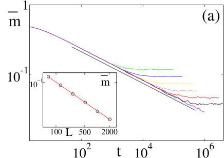
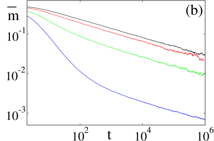
Figure 1: A: Log-log plot of the time decay of the average order-parameter at the critical point, $a_{c}=-0.143668$, for system sizes $2^{6}$, $2^{7}$, $2^{8}$, $2^{9}$, $2^{10}$, $2^{11}$, and $2^{17}$ respectively and $q=3$. In the inset, the average saturation values of the previous curves are plotted as a function of the system-size, $L$, in double-logarithmic scale. B: Averaged order-parameter decay for equation (4) with $q=0.5,1,2,4$ (from bottom to top) in a system of size $L=2^{17}$. For any $q>0$ we observe the same asymptotic decay exponent at the same critical point location.

For other values of $q$ we have verified that, as shown in figure 2, none of the previously reported exponents, nor the location of the critical point, are altered, although $q-$dependent transient effects exist. The invariance of $a_{c}$ against changes in $q$ can be understood from the fact that $a_{c}$ corresponds to the value of $a$ for which depinned interfaces, arbitrarily far from the wall, invert their direction of motion; this is not affected by the nature of the wall, i.e. by the value of $q$.

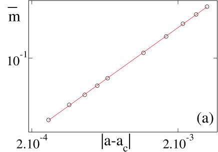
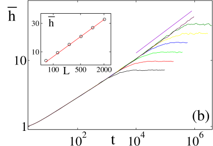
Figure 2: A: Log-log plot of the saturation values of ${\bar{m}}$ for different values of $a$ nearby the critical point. From the slope we estimate $\beta=0.332(5)$. B: Log-log plot of the time growth of the averaged height $h=-\log(n)$ for the same value of $a$ and same system sizes as in figure 1. In the inset, the average saturation values of the previous curves are plotted as a function of the system-size, $L$, in a log-log scale.

Additionally, the order-parameter exponent $\beta\approx 0.332(5)$ has been measured for $L=2^{17}$ (see also figure 2). The previous best estimation was $\beta=0.32(2)$ [7].

We have also studied the scaling properties of the height field ${\bar{h}}=-\overline{\log(n)}$ (see Fig.2(b)). An analysis analogous to that presented above for $m$ leads to ${\bar{h}}(t)\approx t^{0.323(10)}$, ${\bar{h}}\sim|a-a_{c}|^{-0.48(3)}$, and ${\bar{h}}(a_{c},L)\sim L^{0.48(2)}$, which define a set of critical exponents for $h$ analogous to those for $m$ : $\theta_{h}\approx-0.323(10)$, $\beta_{h}\approx-0.48(3)$, and $\beta_{h}/\nu\approx-0.48(2)$ (see figure 2b). The previous best estimations for these exponents were: $-0.355(15)$, $-0.52(2)$ and, $-0.52(2)$ respectively [7]. The minus signs just reflect the fact that ${\bar{h}}$ diverges at the transition point. A summary including our best estimates for the critical exponents can be found in table 1.

$\theta$ $\beta$ $\beta/\nu$ $\nu$ $z$ m 0.229(5) 0.332(5) 0.335(5) 0.99(3) 1.46(5) h -0.323(10) -0.48(3) -0.48(2) 1.0(1) 1.48(10)

Table 1: Critical exponents for the MN2 class in $d=1$ as calculated in this paper. Scaling of saturation times gives $z$ which is consistent with the value $z=\beta/(\theta\nu)$ [3, 4].

Finally, we stress that our results are compatible with the theoretical predictions $z=3/2$ and $\nu=1$, expected to be valid for both MN1 and MN2 [4, 3]. Also, all the standard scaling laws between exponents are satisfied [3].

4 Discussion

We have studied the dynamics of KPZ-like interfaces with $\lambda>0$ bounded by a lower-wall. The results and phenomenology differ from that of upper-walls. By performing a Cole-Hopf or logarithmic transformation, the resulting order-parameter Langevin equation (3) is singular and no satisfying result can be derived from it. Instead, the main result of this paper, is that a sound Langevin equation (4) can be written in terms of a non-order-parameter field which diverges at the transition. For such an equation we have performed (i) a self-consistent mean-field analysis leading to the result $\beta=1/q$, and no trace of any strong-coupling regime (noise-dependent $\beta$ exponent value) contrarily to what happens for the upper-wall case; (ii) extensive numerical integrations of the stochastic equation using a recently introduced very-efficient numerical scheme. The obtained critical exponent values are in good agreement with previously known ones measured in simulations of discrete models, and improve the level of accuracy and precision.

In summary, we have shown that an apparently ill-behaved non-order-parameter Langevin equation constitutes a sound continuous representation of the pinning-depinning transition experienced by interfaces in the Kardar-Parisi-Zhang class under the presence of a bounding lower-wall. Performing further analytical, renormalization group analyses of the present Langevin equation remains as a challenging task.

References

References

- [1] Kardar M, Parisi G and Zhang Y C 1986 Phys. Rev. Lett. 56 889
- [2] Halpin-Healy T and Zhang Y C 1995 Phys. Rep. 254 215 Barabási A L and Stanley H E 1995 Fractal Concepts in Surface Growth (Cambridge: University Press Cambridge) and references therein.
- [3] Muñoz M A 2004 Nonequilibrium Phase Transitions and Multiplicative Noise (Advances in Condensed Matter and Statistical Mechanic) ed E Korutcheva and R Cuerno (New York: Nova Science Publishers) p 34 (Preprint cond-mat/0303650)
- [4] Grinstein G, Muñoz M A and Tu Y 1996 Phys. Rev. Lett. 76 4376
- [5] Tu Y, Grinstein G and Muñoz M A 1997 Phys. Rev. Lett. 78 274
- [6] Muñoz M A and Hwa T 1998 Europhys. Lett. 41 147
- [7] Muñoz M A, de los Santos F and Achahbar A 2003 Braz. J. Phys. 33 443 (Preprint cond-mat/0304239)
- [8] Ahlers V and Pikovsky A 2002 Phys. Rev. Lett. 88 254101 Droz M and Lipowski A 2003 Phys. Rev. E 67 056204 Ginelli F, Ahlers V, Livi R, Mukamel D, Pikovsky A, Politi A, and Torcini A 2003 Phys. Rev. E 68 065102
- [9] Muñoz M A and Pastor Satorras R 2003 Phys. Rev. Lett. 90 204101
- [10] de los Santos F, Telo da Gama M M and Muñoz M A 2002 Europhys. Lett. 57 803 de los Santos F, Telo da Gama M M and Muñoz M A 2003 Phys. Rev. E 67 021607
- [11] Hinrichsen H, Livi R, Mukamel D and Politi A 1997 Phys. Rev. Lett. 79 2710 Hinrichsen H, Livi R, Mukamel D and Politi A 2003 Phys. Rev. E 68 041606
- [12] Kissinger T, Kotowitz A, Kurz O, Ginelli F, and Hinrichsen H 2005 J. Stat. Mech. P06002 (Preprint cond-mat/0503582)
- [13] Indeed, it can be easily shown that a KPZ equation with positive non-linearity and a “lower-wall” is equivalent (can be mapped by changing the sign of ) to a KPZ with a negative non-linearity coefficient and an “upper-wall” [3].
- [14] In the more general case , the different coefficient can be reabsorbed by using .
- [15] The sole difference between utilizing the Ito or the Stratonovich calculus, in this case, is a trivial shift in [16].
- [16] N G van Kampen 1981 Stochastic Processes in Physics and Chemistry (Amsterdam: North-Holland) C W Gardiner 1985 Handbook of Stochastic Methods (Berlin and Heidelberg: Springer Verlag)
- [17] Genovese W and Muñoz M A 1999 Phys. Rev. E 60 69
- [18] Ginelli F and Hinrichsen H 2004 J. Phys. A 37 11085
- [19] In fact, except for the factor in front of equation (3) coincides with the Cole-Hopf transform of that is the growth of wetting layers toward their equilibrium state [Lipowsky R 1985 J. Phys. A 18 L585]. Observe that this is just the equilibrium, Edwards-Wilkinson model, in the presence of a bounding wall. Note also that the factor in equation (3) cannot be readsorbed by reparametrizing.
- [20] Newman T J and Bray A J 1996 J. Phys. A 29 7917 Lam C H and Shin F G 1998 Phys. Rev. E 58 5592
- [21] Muñoz M A, Colaiori F and Castellano C 2005 Mean field approach to systems with multiplicative noise Preprint cond-mat/0506635. To appear in Phys. Rev. E
- [22] Birner T, Lippert K, Müller R, Kühnel A, and Behn U 2002 Phys. Rev. E 65 046110
- [23] Van den Broeck C, Parrondo J M R, Armero J and Hernández Machado A 1994 Phys. Rev. E 49 2639
- [24] For some values of , can be evaluated exactly: immediately leads to and ; for , can be expressed in terms of parabolic-cylinder functions . The asymptotic expansion for large leads to and .
- [25] San Miguel M and Toral R 1997 Stochastic Effects in Physical Systems (Instabilities and Nonequilibrium Structures VI) ed Tirapegui E and Zeller W (Kluwer Academic Publishers) pp 35-130 (Preprint cond-mat/9707147)
- [26] The part of the Langevin equation to be integrated can be written as where is a Wiener process. Since this is interpreted in the Stratonovich sense, we can safely perform the change of variables and obtain . This describes a drifted Brownian motion equation whose solution is given by a normal distribution of mean and variance : . Inverting the change of variables, we are left with a log-normal form, which can be sampled in an exact way by taking: . This same expression can also be derived by changing variables in the Langevin equation, performing one time-step evolution, and changing back variables.
- [27] Dornic I, Chaté H and Muñoz M A 2005 Phys. Rev. Lett. 94 100601 Dornic I, Chaté H and Muñoz M A In preparation Pechenik L and Levine H 1999 Phys. Rev. E 59 3893 Moro E 2004 Phys. Rev. E R 70 045102