Path integral evaluation of the one-loop effective potential in field theory of diffusion-limited reactions

Abstract

The well-established effective action and effective potential framework from the quantum field theory domain is adapted and successfully applied to classical field theories of the Doi and Peliti type for diffusion controlled reactions. Through a number of benchmark examples, we show that the direct calculation of the effective potential in fixed space dimension $d=2$ to one-loop order reduces to a small set of simple elementary functions, irrespective of the microscopic details of the specific model. Thus the technique, which allows one to obtain with little additional effort, the potentials for a wide variety of different models, represents an important alternative to the standard model dependent diagram-based calculations. The renormalized effective potential, effective equations of motion and the associated renormalization group equations are computed in $d=2$ spatial dimensions for a number of single species field theories of increasing complexity.

KEY WORDS: Effective potential, renormalization group, reaction, diffusion.

1 Introduction

The effective potential provides physical insight into the behavior of non-equilibrium stochastic dynamics, and takes into account both nonlinear interactions and random fluctuations to a given number of loops [1]. It has been used to study transitions in non-equilibrium steady states [2] by means of the renormalization group improved equation of state [3], and has been used most recently in nonperturbative renormalization group (RG) methods applied to nonequilibrium critical phenomena [4].

Given the importance of the effective potential in statistical physics, it is useful to have efficient analytic calculational methods for its evaluation that are applicable to a wide variety of non-equilibrium field theories. In this paper, we take the well-established effective action and effective potential formalism from quantum field theory and adapt it to obtain renormalized closed form analytic expressions for the perturbative potential and attendant renormalization group equations (RGE). Once this is carried in detail for one given model, it is easy to extend it to a wide class of different reaction models with little additional effort.

To illustrate and validate these techniques, we will consider some well studied field theories of reaction and diffusion processes that have been derived from the microscopic master equations following the procedures of Doi [5] and Peliti [6]. We will show by explicit example that the method allows one to obtain both renormalized potentials and RGEs with little effort. In fixed dimension, this represents a major advantage over the delicate diagram based approach where each separate reaction model requires defining and handling a distinct set of diagrams and the working out of combinatorics.

We now outline the basic steps that take us from a given bare action to the one-loop effective potential. The field theories we are interested in are characterized by bare (unrenormalized) actions $S[\phi,{\bar{\phi}}]$ that depend on a set of fields $\phi_{i}$, an equal number of response fields ${\bar{\phi}}_{i}$, where $i=(1,2,...,N)$ and $N$ is the number of independent species in the model. From $S$ we construct the following array of second order functional derivatives of the action:

$$S^{(2)}(\phi,{\bar{\phi}};x,y)=\left(\begin{array}[]{cc}\frac{\delta^{2}}{\delta\bar{\phi}_{i}(x,t)\delta\bar{\phi}_{j}(y,s)}&\frac{\delta^{2}}{\delta\bar{\phi}_{i}(x,t)\delta\phi_{j}(y,s)}\\ \frac{\delta^{2}}{\delta\phi_{i}(x,t)\delta\bar{\phi}_{j}(y,s)}&\frac{\delta^{2}}{\delta\phi_{i}(x,t)\delta\phi_{j}(y,s)}\\ \end{array}\right)S[\phi,{\bar{\phi}}],$$ (1)

where $i,j=(1,2,\ldots,N)$. This is written in $2\times 2$ block form. Since the potential is defined for constant and steady field configurations, we easily evaluate the Fourier transform (FT) of Eq. (1) via

$$FT\Big{(}S^{(2)}(\phi,{\bar{\phi}};x,y)\Big{|}_{\phi,{\bar{\phi}}=const.}\Big{)}=M(k,\omega;\phi,{\bar{\phi}})\times(2\pi)^{d+1}\delta^{d}(k-p)\delta(\omega-\Omega),$$ (2)

where $M$ is a $2N\times 2N$ matrix and $d$ is the spatial dimension. We then evaluate the determinant of $M$ and insert it into the expression for the one-loop potential (see the Appendix for a self-contained derivation):

$$\mathcal{V}(\phi,{\bar{\phi}})=V_{0}(\phi,{\bar{\phi}})+\frac{\mathcal{A}}{2}\int\frac{d^{d}k}{(2\pi)^{d}}\,\int_{-\infty}^{\infty}\frac{d\omega}{2\pi}\ln\Big{(}\frac{\det M(k,\omega;\phi,{\bar{\phi}})}{\det M(k,\omega;0,1)}\Big{)}.$$ (3)

Thus, given an action $S[\phi,{\bar{\phi}}]$, it is straightforward to calculate the corresponding matrix $M$, Eq. (2), followed by its determinant, and thence to the effective potential Eq. (3). The zero loop contribution $V_{0}$ corresponds to the non-derivative part of the action $S$ (see Eq. (135)). When this is renormalized, we will refer to it as the tree-level potential. The one loop contribution is proportional to $\mathcal{A}$. The indicated integrations over frequency $\omega$ and wavevector $k$ can be often be expressed entirely in terms of elementary functions for fixed dimension. These points will be demonstrated explicitly in what follows.

Once the effective potential is calculated to some order in perturbation theory or loops, it is a simple matter to obtain the associated RGEs [7]. This procedure for obtaining the RGE’s is based on the so-called derivative technique, which was first introduced in the work of Fujimoto et al. [8] and subsequently extensively developed in [9]. The important observation is that the bare theory does not depend on the arbitrary scale $\mu$ introduced by the renormalization scheme. This observation leads to a simple identity. This identity yields an equation which is a polynomial in the background field whose coefficients are precisely the RGE’s that we seek. This is a very simple and powerful technique that deserves wider use. Equally noteworthy is the fact that to one-loop order, the case we treat here, the analytic calculation of the effective potential is entirely straightforward and one can dispense with model-dependent diagrammatic manipulations. This has the clear advantage of allowing one to survey and analyze comparatively a wide variety of reaction-diffusion models by making simple algebraic substitutions to some of the terms appearing within the universal formula for the one-loop effective potential. Knowledge of the effective potential also allows one to reconstruct the effective action (up to wavefunction renormalization) and deduce the corresponding equations of motion obeyed by the physical density field. These equations of motion are deterministic, yet incorporate the presence of the internal reaction noise through modified effective force terms.

The remainder of this paper is concerned with the explicit evaluation of Eq. (3) for a selected number of single species ($N=1$) diffusion limited reactions in $d=2$, and is organized as follows. In the next Section, we calculate the one-loop effective potential corresponding to pure pair annihilation $A+A\rightarrow\emptyset$. This is renormalized and the resultant finite expression is examined with and without the loop corrections to reveal qualitatively the role of fluctuations on the asymptotic states of the system. With the potential calculated, it is a simple matter to obtain the associated renormalization group equation (RGE) that controls the scale dependence of the annihilation reaction rate. We also derive the effective equation of motion satisfied by the fluctuation averaged particle density. In Sec. 3, we calculate the effective potential for the Gribov process which is described by the set of single species reactions $A\rightarrow\emptyset,A\rightarrow A+A,A+A\rightarrow A$ and extract the one-loop RGE’s and derive the effective equation of motion. Reaction and diffusion systems with the underlying reaction process $A+A\rightarrow\emptyset$ and $A\rightarrow(m+1)A$ are known as branching and annihilating random walks (BARW). Here we calculate the one-loop effective potential for arbitrary even $m$ in Sec. 4 and extract the RGE’s in Sec. 4.2. We then specialize to the case $m=2$, solve the corresponding RGE’s and obtain the equation of motion for the noise-averaged density field. The purpose of this paper is to carry these steps out explicitly in detail in order to illustrate the techniques involved and the ease with which they are applied to a variety of reaction models. Conclusions and discussion are presented in Sec. 5.

2 Pair annihilation reaction $A+A\rightarrow\emptyset$

Perhaps the simplest of all two-body irreversible recombination processes is the single species pair annihilation reaction $A+A\rightarrow{\rm inert}$. In this model, density fluctuations were shown to alter radically the asymptotic decay laws predicted from the mean-field rate equation approach for all dimensions $d\leq 2$ through a series of dimensional considerations, heuristic and scaling arguments and computer simulations [10, 11]. The anomalous scaling in the density was firmly established by Peliti on the basis of field theoretical descriptions using the renormalization group (RG)[12]. Subsequent works applying the RG to this system include [13, 14, 15]. An RG calculation for the reaction $kA\rightarrow{\rm inert}$ is carried out in [16], which recovers Peliti’s result for $k=2$. To illustrate the techniques mentioned above, we present a detailed calculation of the one-loop approximation to the effective potential in this simplest possible case. We renormalize and examine this potential, use it for a simple derivation of the corresponding RGE’s in $d=2$, and to obtain the effective equation of motion for the noise-averaged particle density.

2.1 One loop effective potential

The following bare action will be the starting point for our effective potential calculation:

$$S[\psi,\bar{\psi}]=\int d^{d}x\,dt\left[\bar{\psi}\Big{(}\partial_{t}+\xi-D\nabla^{2}\Big{)}\psi-\lambda\big{(}1-{\bar{\psi}}^{2}\big{)}\psi^{2}\right].$$ (4)

The continuum parameters $D,\lambda$ appearing in the action Eq. (4) stand for particle diffusion and the annihilation reaction rate, respectively. A field-theoretic action $S$ corresponding to the pair annihilation reaction including diffusion was first written down almost twenty years ago by Peliti [12], but without the inclusion of the bare parameter $\xi$. This deserves some special mention. Physically, this is a mass term, and is normally taken identically to zero from the outset in field-theoretic treatments of pair-annihilation. Here, we must explicitly add it to the bare tree-level action Eq. (4), since, as we will demonstrate below, it is required in order to carry out consistently the one-loop renormalization of the effective potential. Nevertheless, after this renormalization is performed, we are free to set the finite and renormalized value of $\xi$ to zero, and we will do so. Our renormalized action agrees with the renormalized action obtained by other means [12].

We next carry out the basic steps outlined above in Sec (1) that take us from the bare action to the formal expression of the one-loop potential. The matrix Eq. (1) of second functional derivatives of the action is

$$S^{(2)}(\phi,{\bar{\phi}}) = \left(\begin{array}[]{cc}2\lambda\phi^{2}&-\partial_{t}+\xi-D\nabla^{2}+4\lambda\bar{\phi}\phi\\ \partial_{t}+\xi-D\nabla^{2}+4\lambda\bar{\phi}\phi&-2\lambda(1-{\bar{\phi}}^{2})\\ \end{array}\right)$$ (7)

$$\times \delta^{d}(x-y)\delta(t-s).$$ (8)

This is a tensor product of a $2\times 2$ matrix in field space times an infinite dimensional but diagonal array in configuration space and in time (the product of delta functions). Since the effective action and potential depend on the averages of the fluctuating fields, we must distinguish between the pairs of fields $\phi$, $\psi$, and $\bar{\phi}$,$\bar{\psi}$, respectively; see Eq. (130). For constant fields we pass to Fourier variables to obtain the array $M$, Eq. (2), where

$$M(k,\omega;\phi,\bar{\phi})=\left(\begin{array}[]{cc}2\lambda\phi^{2}&-i\omega+\xi+Dk^{2}+4\lambda\bar{\phi}\phi\\ +i\omega+\xi+Dk^{2}+4\lambda\bar{\phi}\phi&-2\lambda(1-{\bar{\phi}}^{2})\\ \end{array}\right).$$ (9)

Inserting this matrix into the expression for the one-loop effective potential Eq. (3) yields (recall that $V_{0}=\frac{S}{VT}$ for constant fields)

$$\mathcal{V}(\phi,\bar{\phi})=-\lambda\phi^{2}(1-{\bar{\phi}}^{2})+\xi\bar{\phi}\phi$$

$$+ \frac{\mathcal{A}}{2}\int\frac{d^{d}k}{(2\pi)^{d}}\,\int_{-\infty}^{\infty}\frac{d\omega}{2\pi}\ln\Big{(}\frac{\omega^{2}+[Dk^{2}+\xi+4\lambda\phi\bar{\phi}]^{2}+4\lambda^{2}\phi^{2}(1-{\bar{\phi}}^{2})}{\omega^{2}+[Dk^{2}+\xi]^{2}}\Big{)}.$$

We first carry out the frequency integral, which can be evaluated exactly in closed form. By means of the following identity (see Eq.(4.222.1) of [17]) valid for $C,A>0$

$$\int_{-\infty}^{\infty}d\omega\ln\Big{(}\frac{\omega^{2}+C^{2}}{\omega^{2}+A^{2}}\Big{)}=2\pi\big{(}C-A),$$ (11)

we can write the one-loop $O(\mathcal{A})$ contribution in Eq. (2.1) as follows:

$$\mathcal{I} = \frac{1}{2}\int_{0}^{\infty}k^{d-1}dk\,\int\frac{d\Omega_{d}}{(2\pi)^{d}}\,\left\{\sqrt{(Dk^{2}+\xi+4\lambda\phi\bar{\phi})^{2}+4\lambda^{2}\phi^{2}(1-{\bar{\phi}}^{2})}\right.$$ (12)

$$- \left.\sqrt{(Dk^{2}+\xi)^{2}}\right\},$$

where $d\Omega_{d}$ is the element of solid angle in $d$-dimensional wavevector space. We now temporarily regulate the integral over wavenumber modulus $k$ with an ultraviolet cut-off $k<\Lambda$ and evaluate it directly in $d=2$ dimensions. Introducing the change of variable $u=Dk^{2}$, we can express the regulated $d=2$ integral Eq. (12) as follows:

$$\mathcal{I}_{\Lambda}=\frac{1}{8\pi D}\int_{u=0}^{u=D\Lambda^{2}}du\left\{\sqrt{u^{2}+a_{1}u+a_{2}}-\sqrt{(u+\xi)^{2}}\right\},$$ (13)

where

$$a_{1} = 2(\xi+4\lambda\phi\bar{\phi})$$ (14)

$$a_{2} = \frac{{a_{1}}^{2}}{4}+4\lambda^{2}\phi^{2}(1-{\bar{\phi}}^{2})$$ (15)

$$\Delta = 4a_{2}-a_{1}^{2}=16\lambda^{2}\phi^{2}(1-{\bar{\phi}}^{2}),$$ (16)

and which can be expressed in terms of the following elementary functions (see e.g., (2.262.1) and (2.261) in [17]):

$$(8\pi D)\mathcal{I}_{\Lambda} = \frac{(2D\Lambda^{2}+a_{1})}{4}\sqrt{a_{2}+a_{1}D\Lambda^{2}+(D\Lambda^{2})^{2}}$$

$$+ \frac{\Delta}{8}\ln\Big{(}2\sqrt{a_{2}+a_{1}D\Lambda^{2}+(D\Lambda^{2})^{2}}+2D\Lambda^{2}+a_{1}\Big{)}$$

$$- \frac{1}{2}(D\Lambda^{2}+\xi)^{2}-\frac{a_{1}}{4}\sqrt{a_{2}}+\frac{\xi^{2}}{2}-\frac{\Delta}{8}\ln\big{(}2\sqrt{a_{2}}+a_{1}\big{)}.$$

A careful asymptotic analysis of the regulated loop integral Eq. (2.1) reveals that $\mathcal{I}_{\Lambda}$ contains a quadratic and a logarithmic divergence in $\Lambda$ in addition to certain finite terms as this UV cutoff is taken to infinity, namely

$$\lim_{\Lambda\rightarrow\infty}\mathcal{I}_{\Lambda} = \frac{1}{8\pi D}\left\{\big{(}\frac{a_{1}}{2}-\xi\big{)}(D\Lambda^{2})-\frac{\Delta}{8}\ln\Big{(}\frac{2\sqrt{a_{2}}+a_{1}}{4D\Lambda^{2}}\Big{)}+\frac{1}{16}(\Delta+2a_{1}^{2})\right.$$ (18)

$$- \left.\frac{a_{1}}{4}\sqrt{a_{2}}\right\}+O(\Lambda^{-2}).$$

A particularly useful separation between finite and divergent pieces is obtained by introducing an arbitrary finite momentum scale $\mu$ and writing the argument of the logarithm as follows:

$$\frac{2\sqrt{a_{2}}+a_{1}}{4D\Lambda^{2}}=\frac{2\sqrt{a_{2}}+a_{1}}{4D\mu^{2}}\times\frac{\mu^{2}}{\Lambda^{2}}.$$ (19)

After using this simple identity Eq. (19), we have the following regulated one loop effective potential Eq. (2.1) in $d=2$ space dimensions:

$$\mathcal{V}(\phi,\bar{\phi}) = -\lambda\phi^{2}(1-{\bar{\phi}}^{2})+\xi\phi\bar{\phi}$$ (20)

$$+ \frac{\mathcal{A}}{8\pi D}\left\{\big{(}\frac{a_{1}}{2}-\xi\big{)}(D\Lambda^{2})+\frac{\Delta}{8}\ln\frac{\Lambda^{2}}{\mu^{2}}-\frac{\Delta}{8}\ln\Big{(}\frac{2\sqrt{a_{2}}+a_{1}}{4D\mu^{2}}\Big{)}\right.$$

$$+ \left.\frac{1}{16}(\Delta+2a_{1}^{2})-\frac{a_{1}}{4}\sqrt{a_{2}}\right\}+O(\Lambda^{-2}).$$

This expression is given in terms of bare (unrenormalized) parameters $(\lambda,\xi)$ and the dependence on the UV cutoff $\Lambda$ is explicit. As pointed out above, the tree-level term $\xi\phi\bar{\phi}$ will be needed for the renormalization program. Note that the regulated effective potential Eq. (20), is seen by inspection (due to elementary properties of the logarithm function) to be manifestly independent of the arbitrary scale $\mu$. This is the key observation needed in order to derive the RGE’s, of which we will make direct use of below.

We now proceed to renormalize, i.e., absorb the divergences into the bare parameters $\lambda$ and $\xi$. To carry this out, we write

$$\lambda = \lambda(\mu)+\mathcal{A}\kappa_{1}+O(\mathcal{A}^{2})$$ (21)

$$\xi = \xi(\mu)+\mathcal{A}\kappa_{2}+O(\mathcal{A}^{2}),$$ (22)

in which we decompose each bare parameter into a finite renormalized and possibly $\mu$-dependent part plus a divergent counterterm. Note the divergent counterterms start off at order $O(\mathcal{A})$, which is the same order at which the divergences in the regulated potential appear. These counterterms $\kappa_{1},\kappa_{2}$ are chosen to render the one-loop effective potential finite and UV-cutoff independent. Note the very important fact that the stochastic fluctuations induce divergent terms at the one-loop level whose coefficients have identical polynomial field structure (namely, $\frac{a_{1}}{2}-\xi$ and $\Delta$, see Eq. (14) and Eq. (16)) as those appearing in the bare tree-level potential $V_{0}$. Inserting Eq. (21,22) into Eq. (20) yields the solution for the two counterterms:

$$\kappa_{1} = +\frac{\lambda^{2}(\mu)}{4\pi D}\ln\frac{\Lambda^{2}}{\mu^{2}}$$ (23)

$$\kappa_{2} = -\frac{\lambda(\mu)}{2\pi}\Lambda^{2}.$$ (24)

In this final step, and after cancelling off the UV divergences, we obtain the finite and renormalized one-loop effective potential for pair-annihilation (in $d=2$):

$$\mathcal{V}(\phi,\bar{\phi}) = -\lambda(\mu)\phi^{2}(1-{\bar{\phi}}^{2})$$ (25)

$$+ \frac{\mathcal{A}}{8\pi D}\Big{\{}-2\lambda^{2}(\mu)\phi^{2}(1-{\bar{\phi}}^{2})\ln\Big{(}\frac{\lambda(\mu)\phi\sqrt{1+3{\bar{\phi}}^{2}}+2\lambda(\mu)\phi\bar{\phi}}{D\mu^{2}}\Big{)}$$

$$+ \lambda^{2}(\mu)\phi^{2}(1-{\bar{\phi}}^{2})+8\lambda^{2}(\mu)\phi^{2}{\bar{\phi}}^{2}-4\lambda^{2}(\mu)\phi^{2}\bar{\phi}\sqrt{1+3{\bar{\phi}}^{2}}\,\,\Big{\}}$$

$$+ O(\mathcal{A}^{2}).$$

We are now free to assign zero to the finite renormalized value of $\xi$, and have done so here and in the following subsections. Below, when we come to discuss the RGE’s, we will see that the renormalized parameter $\xi$ does not run with scale, at least to one-loop order, proving that this is a valid choice. In this expression Eq. (25) it is understood that $\lambda\equiv\lambda(\mu)$ is the renormalized, $\mu$-dependent coupling and we have set the finite renormalized value of $\xi(\mu)$ identically to zero. We next determine their scale dependences.

2.2 The one-loop RGEs

Since the bare theory Eq. (20) does not depend on the arbitrary scale $\mu$ introduced by the renormalization scheme (recall our use of the trivial identity in Eq. (19)), we are able to derive the renormalization group equation that the coupling $\lambda(\mu)$ must satisfy, from the identity [7, 8, 9]

$$\mu\frac{d\mathcal{V}(\phi,\bar{\phi})}{d\mu}=0,$$ (26)

which upon inserting Eq. (25) immediately yields the RGE. Differentiating as indicated, we get

$$0 = \mu\frac{d}{d\mu}\Big{(}-\lambda\phi^{2}(1-{\bar{\phi}}^{2})\Big{)}$$ (27)

$$+ \frac{\mathcal{A}}{8\pi D}\mu\frac{d}{d\mu}\Big{(}-2\lambda^{2}\phi^{2}(1-{\bar{\phi}}^{2})\ln\big{(}\frac{\lambda\phi\sqrt{1+3{\bar{\phi}}^{2}}+2\lambda\phi\bar{\phi}}{D\mu^{2}}\big{)}$$

$$+ \lambda^{2}\phi^{2}(1-{\bar{\phi}}^{2})+8\lambda^{2}\phi^{2}{\bar{\phi}}^{2}-4\lambda^{2}\phi^{2}\bar{\phi}\sqrt{1+3{\bar{\phi}}^{2}}\Big{)}+O(\mathcal{A}^{2}),$$

which implies

$$\mu\frac{d}{d\mu}\Big{(}\lambda\phi^{2}(1-{\bar{\phi}}^{2})\Big{)}=\frac{\mathcal{A}}{2\pi D}\lambda^{2}\phi^{2}(1-{\bar{\phi}}^{2})+O(\mathcal{A}^{2}).$$ (28)

Note that derivatives with respect to $\mu$ of the other terms on the right hand side of Eq. (27) proportional to $\mathcal{A}$ lead to contributions at the next higher order $O(\mathcal{A}^{2})$, and so can be neglected at the one-loop order we are working at. Indeed, from Eq. (21) we see that $d\lambda(\mu)/{d\mu}=d(\lambda-\mathcal{A}\kappa_{1}(\mu))/d\mu=-\mathcal{A}d\kappa_{1}(\mu)/d\mu=O(\mathcal{A}^{2})$.

Cancelling the common field-dependent factor $\phi^{2}(1-{\bar{\phi}}^{2})$ from both sides of Eq. (28) yields the RGE for $\lambda$ in $d=2$:

$$\mu\frac{d\lambda}{d\mu}=\frac{\mathcal{A}}{2\pi D}\lambda^{2},$$ (29)

valid to one-loop order. This can be solved immediately and gives

$$\lambda(\mu) = \lambda_{0}\Big{(}1-\frac{\mathcal{A}\lambda_{0}}{2\pi D}\ln\frac{\mu}{\mu_{0}}+O(\mathcal{A}^{2})\Big{)}^{-1}$$ (30)

$$\approx \lambda_{0}\Big{(}1+\frac{\mathcal{A}\lambda_{0}}{2\pi D}\ln\frac{\mu}{\mu_{0}}\Big{)}+O(\mathcal{A}^{2}),$$

where $\lambda_{0}\equiv\lambda(\mu_{0})$, is the value of the coupling at some initial arbitrary reference scale $\mu_{0}$.

If we retain the dependence on the renormalized $\xi$ in Eq. (25) and deduce the consequences following from Eq. (26), we now obtain two RGE’s, corresponding to the two independent polynomial terms $\phi^{2}(1-{\bar{\phi}}^{2})$ and $\bar{\phi}\phi$, respectively. Once again, we obtain Eq. (29) as well as

$$\mu\frac{d\xi}{d\mu} = 0+O(\mathcal{A}^{2}),$$ (31)

$$\xi(\mu) = \xi(0)+O(\mathcal{A}^{2}),$$

indicating that the parameter $\xi$ does not run with scale, at least to one-loop order. So, it is consistent to take the renormalized (but not the bare) mass parameter to be strictly constant, and setting $\xi(\mu)=\xi(0)=0$ is a perfectly valid choice.

This RGE Eq. (29) has been calculated directly in $d=2$, which coincides of course with the upper critical dimension of the pair-annihilation process [11]. When working with the RG, it is useful to have knowledge of the scale dependence in variable dimension $d$. This would require us to go back and attempt to calculate the potential also in arbitrary $d$, which is a difficult task. This is because the one loop potential represents an infinite sum of Feynman diagrams. While individual diagrams are usually easy to analytically continue to arbitrary dimensions, their infinite sums are not. However, we can gain some useful insight into the structure that the variable-$d$ RGE must have by using some simple dimensional analysis in conjuntion with the $d=2$ RGE in Eq. (29). In this way, we arrive at the approximate mathematical form of the RGE for the dimensionless coupling, which may be expected to hold for values of $d$ close to $d=2$. We comment below in what sense it is approximate. In regards the scaling dimensions of the field theory, the diffusion constant $D$ can be absorbed into a rescaling of the time $t\rightarrow Dt$. Doing so in the action Eq. (4) and expressing the dimensions of the resultant terms in the action in powers of momentum yields [16]

$$[t]=p^{-2}\qquad[\bar{\psi}]=p^{0}\qquad[\psi]=p^{d}\qquad[\xi/D]=p^{2}\qquad[\lambda/D]=p^{2-d}.$$ (32)

From the last equality in Eq. (32), we are lead to define a dimensionless coupling $g$ in any $d$ via

$$g=\frac{\lambda}{D\mu^{\epsilon}},$$ (33)

where $\epsilon=2-d$.

We can write Eq. (29) so that it is dimensionally consistent for all dimensions $d$. This is achieved by first noting that (we set $\mathcal{A}=1$ in what follows)

$$\mu\frac{d\lambda}{d\mu}=\Big{(}\frac{K_{d}}{D\mu^{\epsilon}}\Big{)}_{d=2}\lambda^{2},$$ (34)

where

$$K_{d}=\int\frac{d\Omega_{d}}{(2\pi)^{d}}=[\Gamma(d/2)\pi^{d/2}2^{d-1}]^{-1}$$ (35)

is a geometric factor that results from the integration over solid angles and which is part of the complete $d$-dimensional loop integral in Eq. (12). Note that $K_{2}=\frac{1}{2\pi}$ and that $g(d=2)=\frac{\lambda}{D}$. We next extend Eq. (34) to all dimensions by writing

$$\mu\frac{d\lambda}{d\mu}=\frac{K_{d}}{D\mu^{\epsilon}}\lambda^{2}.$$ (36)

This equation is of course only true in $d=2$, and the approximation comes in using dimensional analysis to extend it to any dimension. Lastly, substituting Eq. (33) into Eq. (36), and expressing $\lambda$ in terms of $g$, yields the (admittedly approximate) one loop beta function for $g$:

$$\beta(g)\equiv\mu\frac{dg}{d\mu}=-\epsilon g+K_{d}\,g^{2}.$$ (37)

This beta function Eq. (37) is quadratic in $g$ and for $d<2$ has the nontrivial fixed point $\beta(g^{*})=0$ at $g^{*}=\frac{\epsilon}{K_{d}}=O(\epsilon)$. This fixed point is of order $\epsilon$. For $d>2$, $g^{*}=0$. Inspection of Eq. (12) shows that the calculation of the one-loop RGE for $\lambda$ valid for arbitrary $d$ would require the integration of the corresponding integrand over the modulus of $k$ with weight $k^{d-1}$, in addition to the integration over solid angle Eq. (35). The above result takes the latter in to account, but the former is evaluated at fixed $d=2$, so we can expect the overall numerical coefficient of the quadratic $g^{2}$ term to be in error in this respect. Nevertheless, for values of $d$ sufficiently close to $d=2$, this should provide qualitatively correct results. By way of comparison, the exact one-loop beta function calculated in [16] is given by

$$\beta(g)=-\epsilon g+\frac{\Gamma(2-d/2)}{2\pi}g^{2}.$$ (38)

For $d>2$, $g^{*}=0$. For $d<2$ the nontrivial fixed point is given by $g^{*}_{L}=\frac{2\pi\epsilon}{\Gamma(2-d/2)}$. At $d=2$, these two beta functions Eq. (37) and Eq. (38) are identical, and we have $\beta(g)=\frac{1}{2\pi}g^{2}$. For $d<2$ we can compare the deviation of the approximate to exact nontrivial fixed point via the ratio $g^{*}/g^{*}_{L}=\frac{\Gamma(2-d/2)}{2\pi K_{d}}$.

2.3 Effective equation of motion

From the one-loop potential we can construct the effective action to the same (one-loop) order via [18, 19, 20, 21, 22]

$$\Gamma[\phi,\bar{\phi}]=\int d^{d}x\,dt\,\left\{Z^{1/2}{\bar{Z}}^{1/2}\bar{\phi}(\partial_{t}-D\nabla^{2})\phi+{\cal V}(\phi(x,t),\bar{\phi}(x,t))+\ldots\right\},$$ (39)

where $Z$ and $\bar{Z}$ denote the wavefunction renormalization constants for $\phi$ and $\bar{\phi}$, respectively, and the dots represent higher derivative terms in the fields. From the fact that there is no wavefunction renormalization for pair-annihilation [6, 16], we can immediately set $Z=\bar{Z}=1$ in Eq. (39). Then, from Eq. (132) and Eq. (25), we can derive the (one-loop) effective equations of motion for pair-annihilation in $d=2$ obeyed by the noise-averaged fields $\bar{\phi}(x,t)=\langle\bar{\psi}(x,t)\rangle_{(0,0)}$ and $\phi(x,t)=\langle\psi(x,t)\rangle_{(0,0)}$. We find that the equation of motion for $\bar{\phi}$ (recall $N=1$)

$$\Big{(}\frac{\delta\Gamma[\phi,\bar{\phi}]}{\delta\phi}\Big{)}\Big{|}_{\phi,\bar{\phi}}=0,$$ (40)

is identically solved by the stationary and homogeneous solution $\bar{\phi}=1$. The equation of motion of the physical density field $\phi$ follows from

$$\Big{(}\frac{\delta\Gamma[\phi,\bar{\phi}]}{\delta\bar{\phi}}\Big{)}\Big{|}_{\phi,\bar{\phi}=1}=0,$$ (41)

which when written out explicitly, implies that

$$\big{(}\partial_{t}-D\nabla^{2}\big{)}\phi = -\frac{\partial\mathcal{V}}{\partial\bar{\phi}}\Big{|}_{\bar{\phi}=1}$$

$$= -2\lambda\phi^{2}-\frac{\cal{A}}{2\pi D}\lambda^{2}\phi^{2}\ln\Big{(}\frac{4\lambda\phi}{D\mu^{2}}\Big{)}+O({\cal A}^{2})$$

$$= F_{\phi}.$$

Here, the effective force experienced by the field $\phi$ is denoted by $F_{\phi}=-\frac{\partial\mathcal{V}}{\partial\bar{\phi}}$. In Fig. 1 we show a qualitative example of the force experienced by the density field $\phi$. Notice that since the recovery force is less strong in the renormalized case (the fluctuations cause the slope at the origin to be less negative, relative to the tree-level case), the rate of approach to the origin will be slower. Putting $\mathcal{A}=0$ on the right hand side of Eq. (2.3) yields the so-called rate equation which one might write down as a first approximation to the equation of motion for the density. If we let $n(t)$ be the spatial average of $\phi$, then we see that the only stationary solution of Eq. (2.3) is $n=0$, corresponding to the inactive state with no particles remaining, which of course, comes as no surprise. Zeroes of the effective force correspond to maxima/minima of the effective potential. Therefore, since the logarithm of a small number is negative, it appears as though the one-loop correction in Eq. (2.3) has turned the minimum at the origin into a maximum and caused a new minimum to appear away from the origin, corresponding to a putative noise induced active state. However, it is wise to proceed with caution in this specific example: the apparent new minimum occurs at a value of $n$ determined by (note from Eq. (32) that the ratios $\lambda/D$ and $n/\mu^{2}$ are pure dimensionless numbers in $d=2$)

$$\Big{(}\frac{\lambda}{D}\Big{)}\ln\Big{(}\frac{4\lambda n}{D\mu^{2}}\Big{)}=-4\pi.$$ (43)

Since we expect higher orders in perturbation theory to bring in higher powers of $(\lambda/D)\ln\big{(}4\lambda n/D\mu^{2}\big{)}$, this new state lies well outside the expected range of validity of the one-loop approximation [22], even for arbitrarily small reaction rates (or large diffusions) $\lambda/D$. This new solution Eq. (43) must be rejected as an artefact of the approximation . Higher loops are needed to assess the situation. However, this same criticism can not be applied to the effective force associated with the Gribov process, the next example to be considered below.

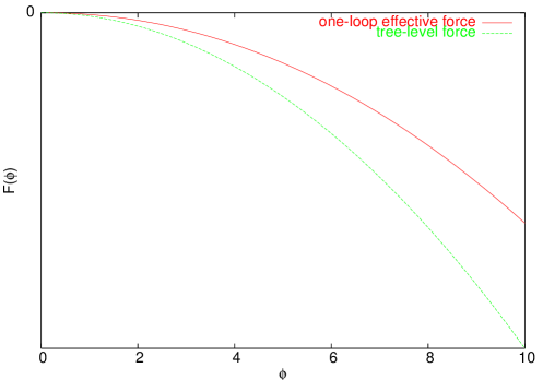
Figure 1: One-loop effective and tree-level force $F(\phi)$. The zero at the origin corresponds to the inactive state.

3 Gribov process $A\rightarrow\emptyset,A\rightarrow A+A,A+A\rightarrow A$

As a second application of the methods outlined in Sec (1), we consider the competing reactions of single particle annihilation, splitting and two-body recombination. This is a simple model exhibiting a non-equilibrium phase transition between active and inactive or absorbing stationary states in which the stochastic fluctuations cease entirely. A mathematical equivalence between such chemical processes and Reggeon field theory has been firmly established [23, 24]. Below we calculate the corresponding one-loop potential, carry out the renormalization and obtain and solve the RGE’s for the rates of pair recombination and fission directly in $d=2$ dimensions.

3.1 One loop effective potential

The following field-theoretic bare (unrenormalized) action $S$ will be the starting point for our effective potential calculation:

$$S[\psi,\bar{\psi}] = \int d^{d}x\,dt\left[\bar{\psi}\Big{(}\partial_{t}+\xi-D\nabla^{2}\Big{)}\psi+\sigma\big{(}1-{\bar{\psi}}\big{)}\bar{\psi}\psi-r\big{(}1-{\bar{\psi}}\big{)}\psi\right.$$ (44)

$$- \left.\lambda\big{(}1-{\bar{\psi}}\big{)}{\bar{\psi}}\psi^{2}+b\bar{\psi}+a\right].$$

The continuum parameters $D,\lambda$ appearing in this action stand for particle diffusion and the reaction rate for two-body recombination ($A+A\rightarrow A$), respectively. The parameter $\sigma$ is the rate of reproduction or fission ($A\rightarrow A+A$) and $r$ is the particle decay rate ($A\rightarrow\emptyset$). Similarly to the pair-annihilation case worked out above, the additional bare terms parametrized by $\xi$, $b$ and $a$ that we have introduced in Eq. (44), will be required in order to carry out consistently the one-loop renormalization of the effective potential. Nevertheless, after this renormalization is performed, we are free to set the finite and renormalized values of all these couplings identically to zero: $\xi=b=a=0$. We will so do in the final renormalized expression for the effective potential obtained below. Once these taken to be zero, the renormalized action (44) will correspond to the Gribov process [25].

Evaluating the array in (1) for this action, taking constant fields and then evaluating the Fourier transform yields the following matrix (note this is independent of both $a$ and $b$)

$$M(k,\omega;\phi,\bar{\phi})_{11} = -2\sigma\phi+2\lambda\phi^{2}$$ (45)

$$M(k,\omega;\phi,\bar{\phi})_{12} = -i\omega+\xi+Dk^{2}+\sigma+r-2\sigma\bar{\phi}-2\lambda\phi(1-2\bar{\phi})$$ (46)

$$M(k,\omega;\phi,\bar{\phi})_{21} = M^{*}(k,\omega;\phi,\bar{\phi})_{12}$$ (47)

$$M(k,\omega;\phi,\bar{\phi})_{22} = -2\lambda(1-{\bar{\phi}})\bar{\phi}.$$ (48)

Inserting this matrix into the expression for the one-loop effective potential Eq. (3) yields

$$\mathcal{V}(\phi,\bar{\phi}) = \sigma(1-\bar{\phi})\bar{\phi}\phi-r\phi(1-\bar{\phi})-\lambda(1-\bar{\phi})\bar{\phi}\phi^{2}+\xi\bar{\phi}\phi+b\bar{\phi}+a$$ (49)

$$+ \frac{\mathcal{A}}{2}\int\frac{d^{d}k}{(2\pi)^{d}}\,\int_{-\infty}^{\infty}\frac{d\omega}{2\pi}\ln\Big{(}\frac{\det M(k,\omega;\phi,{\bar{\phi}})}{\det M(k,\omega;0,1)}\Big{)},$$

where,

$$-\det M(k,\omega;\phi,{\bar{\phi}}) = \omega^{2}+[Dk^{2}+\xi+\sigma+r-2\sigma\bar{\phi}-2\lambda\phi(1-2\bar{\phi})]^{2}$$ (50)

$$+ 2\lambda\bar{\phi}(1-\bar{\phi})(-2\sigma\phi+2\lambda\phi^{2}),$$

$$-\det M(k,\omega;0,1) = {\omega^{2}+[Dk^{2}+\xi-\sigma+r]^{2}}.$$ (51)

The frequency integration in Eq. (49) is again performed immediately using Eq. (11). We regulate and evaluate the remaining wavenumber integral directly in $d=2$ as above in Sec. (2.1). The integral that is needed is similar in structure to that worked out in Eq. (13). After some algebra, we find that the UV-regulated integral takes a form identical to that in Eq. (18). Put $f=\xi+r+\sigma$, then for the bare action Eq. (44) we have $I_{\Lambda}$ as written in Eq. (18), where now the coefficients turn out to be

$$a_{1} = 2\big{(}f-2\sigma\bar{\phi}-2\lambda\phi(1-2\bar{\phi})\big{)}$$ (52)

$$a_{2} = [f-2\sigma\bar{\phi}-2\lambda\phi(1-2\bar{\phi})]^{2}+2\lambda\bar{\phi}(1-\bar{\phi})(-2\sigma\phi+2\lambda{\phi}^{2})$$ (53)

$$\Delta = 4a_{2}-a_{1}^{2}=-16\lambda\sigma(1-\bar{\phi})\bar{\phi}\phi+16\lambda^{2}(1-\bar{\phi})\bar{\phi}\phi^{2}.$$ (54)

At this point we have the following regulated one loop effective potential for the Gribov process (where $F=\xi-\sigma+r$)

$$\mathcal{V}(\phi,\bar{\phi}) = \sigma(1-\bar{\phi})\bar{\phi}\phi-r\phi(1-\bar{\phi})-\lambda(1-\bar{\phi})\bar{\phi}\phi^{2}+b\bar{\phi}+\xi\phi\bar{\phi}+a$$ (55)

$$+ \frac{\mathcal{A}}{8\pi D}\Big{\{}\big{(}\frac{a_{1}}{2}-F\big{)}(D\Lambda^{2})+\frac{\Delta}{8}\ln\frac{\Lambda^{2}}{\mu^{2}}-\frac{\Delta}{8}\ln\Big{(}\frac{2\sqrt{a_{2}}+a_{1}}{4D\mu^{2}}\Big{)}$$

$$+ \frac{1}{16}(\Delta+2a_{1}^{2})-\frac{a_{1}}{4}\sqrt{a_{2}}\Big{\}}+O(\Lambda^{-2}).$$

This expression is given in terms of bare (unrenormalized) parameters $(\sigma,r,\lambda,\xi,b,a)$ and the dependence on the UV cutoff $\Lambda$ is explicit. As remarked above, the terms proportional to $b\bar{\phi}$, $\xi\phi\bar{\phi}$ and the constant $a$ will be needed for carrying out the renormalization program. Note that the regulated effective potential Eq. (55) is independent of the arbitrary scale $\mu$.

We now proceed to renormalize, i.e., absorb the divergences into the bare parameters . Specifically, we write

$$\sigma = \sigma(\mu)+\mathcal{A}\kappa_{1}+O(\mathcal{A}^{2})$$ (56)

$$r = r(\mu)+\mathcal{A}\kappa_{2}+O(\mathcal{A}^{2})$$ (57)

$$\lambda = \lambda(\mu)+\mathcal{A}\kappa_{3}+O(\mathcal{A}^{2})$$ (58)

$$\xi = \xi(\mu)+\mathcal{A}\kappa_{4}+O(\mathcal{A}^{2})$$ (59)

$$b = b(\mu)+\mathcal{A}\kappa_{5}+O(\mathcal{A}^{2})$$ (60)

$$a = a(\mu)+\mathcal{A}\kappa+O(\mathcal{A}^{2}).$$ (61)

The divergent coefficients $\kappa_{i}$ of the counterterms are chosen to cancel off the divergences in the one loop regulated contribution Eq. (55). Inserting Eq. (56-61) into Eq. (55) yields the solutions

$$\kappa_{1} = \frac{\lambda(\mu)\sigma(\mu)}{4\pi D}\ln\frac{\Lambda^{2}}{\mu^{2}}$$ (62)

$$\kappa_{2} = \kappa_{4}=-\frac{\lambda(\mu)}{4\pi}\Lambda^{2}$$ (63)

$$\kappa_{3} = \frac{\lambda^{2}(\mu)}{4\pi D}\ln\frac{\Lambda^{2}}{\mu^{2}}$$ (64)

$$\kappa_{5} = -\kappa=\frac{\sigma(\mu)}{4\pi}\Lambda^{2}.$$ (65)

After this step, we obtain the finite and renormalized one-loop effective potential for the Gribov process in $d=2$:

$$\mathcal{V}(\phi,\bar{\phi}) = \sigma(1-\bar{\phi})\bar{\phi}\phi-r\phi(1-\bar{\phi})-\lambda(1-\bar{\phi})\bar{\phi}\phi^{2}$$ (66)

$$+ \frac{\mathcal{A}}{8\pi D}\Big{\{}\big{[}2\lambda\sigma(1-\bar{\phi})\bar{\phi}\phi-2\lambda^{2}(1-\bar{\phi})\bar{\phi}\phi^{2}\big{]}\times\ln\Big{(}\frac{2\sqrt{a_{2}}+a_{1}}{4D\mu^{2}}\Big{)}$$

$$+ \frac{1}{16}(\Delta+2a_{1}^{2})-\frac{a_{1}}{4}\sqrt{a_{2}}\Big{\}}+O(2\,\,loops).$$

The parameters appearing in this expression (and within $a_{1},a_{2}$ and $\Delta$) are understood here to be the finite scale-dependent ones, that is, $\sigma(\mu),r(\mu)$ and $\lambda(\mu)$. Their explicit scale-dependence is determined below. As we mentioned above, we have set the finite renormalized values of $\xi$, $b$ and $a$ identically to zero in this final expression for the potential.

3.2 The one-loop RGEs

Since $\mathcal{V}(\phi,\bar{\phi})$ does not depend on the arbitrary scale $\mu$, inserting Eq. (66) into Eq. (26) will immediately yield the one-loop renormalization group equations in $d=2$:

$$\mu\frac{d\sigma}{d\mu} = \frac{\mathcal{A}}{2\pi D}\sigma\lambda$$ (67)

$$\mu\frac{dr}{d\mu} = 0+O(\mathcal{A}^{2})$$ (68)

$$\mu\frac{d\lambda}{d\mu} = \frac{\mathcal{A}}{2\pi D}\lambda^{2}.$$ (69)

As we saw above in Sec. (2.2), the one-loop RGE’s follow simply from differentiating the explicit $\mu$-dependence in the logarithm term. The above three RGEs result from the vanishing of the individual coefficients of the independent field polynomials $(1-\bar{\phi})\bar{\phi}\phi$, $(1-\bar{\phi})\phi$ and $(1-\bar{\phi})\bar{\phi}\phi^{2}$, respectively. These equations can be solved immediately and give

$$\sigma(\mu) = \sigma_{0}\big{(}\frac{\mu}{\mu_{0}}\big{)}^{\frac{\mathcal{A}\lambda_{0}}{2\pi D}}\exp\big{(}O(\mathcal{A}^{2})\big{)}$$ (70)

$$r(\mu) = r_{0}+O(\mathcal{A}^{2})$$ (71)

$$\lambda(\mu) = \lambda_{0}\Big{(}1-\frac{\mathcal{A}\lambda_{0}}{2\pi D}\ln\frac{\mu}{\mu_{0}}+O(\mathcal{A}^{2})\Big{)}^{-1}.$$ (72)

If we retain the dependence of Eq. (66) on the other three parameters $\xi$, $b$ and $a$ and work out the consequences implied by Eq. (26), we would find that they satisfy RGEs similar to that for $r$ in Eq. (68). We conclude that neither $\xi$, $b$ nor $a$ run with scale (at one-loop order). So, we are justified in setting $\xi(\mu)=b(\mu)=a(\mu)=0$ after the renormalization procedure is properly carried out.

Although the RGE’s in Eq. (67,69) have been calculated directly in $d=2$ dimensions, as in Sec. (2.2) simple dimensional analysis can be exploited in order to infer the approximate form that these equations will take in other dimensions. Dimensional analysis of the action Eq. (44) yields (and after absorbing the diffusion constant $D$ by a re-scaling of the time)

$$[t] = p^{-2}\qquad[\bar{\psi}]=p^{0}\qquad[\psi]=p^{d}\qquad[\sigma/D]=p^{2},$$ (73)

$$[\mu/D]=[r/D]=[\xi/D]=p^{2}\qquad[\lambda/D]=p^{2-d}.$$

From these relations, we are led to introduce the two dimensionless parameters ($\epsilon=2-d$)

$$s=\frac{\sigma}{D\mu^{2}}\qquad g=\frac{\lambda}{D\mu^{\epsilon}}.$$ (74)

We now write Eq. (67) and Eq. (69) so they are dimensionally correct, albeit only approximate in any dimension $d$ (we herewith set $\mathcal{A}=1$):

$$\mu\frac{d\sigma}{d\mu} = \frac{K_{d}}{D\mu^{\epsilon}}\sigma\lambda$$ (75)

$$\mu\frac{d\lambda}{d\mu} = \frac{K_{d}}{D\mu^{\epsilon}}\lambda^{2},$$ (76)

where $K_{d}$ is defined in Eq. (35). Inserting $s$ and $g$ from Eq. (74) into Eq. (75) and Eq. (76) yields the following (approximate if $d\neq 2$) one-loop beta and flow functions

$$\beta(g) = \mu\frac{dg}{d\mu}=-\epsilon g+K_{d}\,g^{2}$$ (77)

$$\gamma(s) = \mu\frac{d\ln(s)}{d\mu}=-2+K_{d}\,g.$$ (78)

3.3 Effective equation of motion

Just as for the case of pair annihilation treated above, we can recover the effective action from knowledge of the effective potential and obtain the noise-corrected equations of motion for the Gribov process. Inserting Eq. (66) into Eq. (39), we again find that $\bar{\phi}=1$ solves Eq. (40) identically while the equation of motion for $\phi$ Eq. (41)–the noise-averaged particle density– works out to be

$$\big{(}\partial_{t}-D\nabla^{2}\big{)}\phi = -\frac{\partial\mathcal{V}}{\partial\bar{\phi}}\Big{|}_{\bar{\phi}=1}$$

$$= \sigma\phi-r\phi-\lambda\phi^{2}$$

$$+ \frac{\cal{A}}{4\pi D}(\lambda\sigma\phi-\lambda^{2}\phi^{2})\ln\Big{(}\frac{r-\sigma+2\lambda\phi}{D\mu^{2}}\Big{)}+O({\cal A}^{2})$$

$$= F_{\phi}.$$

In Fig. 2 we show an example of the force experienced by the field $\phi$ for a case with $r<\sigma$ and equilibrium density $\phi=(\sigma-r)/\lambda$. Setting $\mathcal{A}=0$ on the right hand side of Eq. (3.3) yields the so-called rate equation which one might write down as a first approximation to the equation of motion for the density. If we let $n(t)$ stand for the spatial average of $\phi$, then we see that the only stationary solutions of Eq. (3.3) for zero noise are $n=0$, corresponding to the inactive state with no particles remaining, and $n$ = $\frac{\sigma-r}{\lambda}$, the active state, provided of course that $\sigma>r$. Notice that for $\phi<(\sigma-r)/2\lambda$ the effective renormalized force is ill-defined (it becomes complex, due to the logarithm term in the renormalized expression). But suppose that we arrange for the system to have initially equal rates of fission and decay: $\sigma=r$. Then in the absence of noise, the only stationary solution of Eq. (3.3) at tree-level is the inactive state $n=0$ (see Fig 2-right, tree-level force). However, the situation changes once the one-loop correction is included. Even when $\sigma=r$, there can be noise-induced active states, corresponding to finite positive values of $n$, which are given implicitly by the transcendental equation

$$n=\frac{(\sigma-\lambda n)}{4\pi D}\,\ln\Big{(}\frac{2\lambda n}{D\mu^{2}}\Big{)}.$$ (80)

See the transitions to case 1 $(\sigma/D=13.8)$ and to case 2 $(\sigma/D=15.5)$. Since the physical density must be nonnegative, for Eq. (80) to have positive solutions $n>0$ requires that either (i) $\sigma>\lambda n>D\mu^{2}/2$ or (ii) $\sigma<\lambda n<D\mu^{2}/2$. In the first case, we are in effect canceling a term of order unity against a term of order $\sigma$, and there is no reason why $\sigma$ need be small: we are not employing $\sigma$ as a perturbation expansion parameter. Thus the finite density solutions satisfying criteria (i) can be valid in the context of perturbation theory. The solutions satisfying criteria (ii) however fall prey to the same criticism as the solution given in Eq. (43). In latter case, we are in effect cancelling a term of order $\lambda$ against a term of order $\lambda^{2}$.

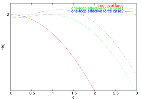
Figure 2: One-loop effective and tree-level force $F(\phi)$. Depending on the values of renormalized model parameters $\sigma(\mu),\lambda(\mu)$, the noise can change the number of zeroes in the force from the one at the origin (tree-level force) to two (case 1) to three (case 2). Zeroes at finite $\phi$ signal the presence of active states.

4 Branching and annihilating random walk $A+A\rightarrow\emptyset$ and $A\rightarrow(m+1)A$

In our third and final application of these calculational methods, we calculate the renormalized one-loop effective potential for field theories of branching and annihilating random walks (BARW). BARW describe the dynamics of a single particle undergoing three basic processes: diffusion, an annihilation reaction $A+A\rightarrow\emptyset$ and a branching process $A\rightarrow(m+1)A$, where $m$ is a positive integer. A field theory for these processes was constructed and its asymptotic properties analyzed in [26], where further references on BARW can be found. Below we deduce the corresponding RGE’s in $d=2$ dimensions for any even $m$ and then specialize to the case $m=2$ and solve them. The associated one-loop potential and effective force are plotted which show qualitatively the role of small amplitude noise on the system.

4.1 One loop effective potential

The field theoretic action for even-$m$ BARW we will use in the following calculations is adapted from [26] and reads as follows:

$$S[\psi,\bar{\psi}] = \int d^{d}x\,dt\left[\bar{\psi}\Big{(}\partial_{t}+\xi-D\nabla^{2}\Big{)}\psi-\lambda\big{(}1-{\bar{\psi}}^{2}\big{)}\psi^{2}\right.$$

$$+ \left.\sum_{l=1}^{m/2}\sigma_{2l}(1-{\bar{\psi}}^{2l})\bar{\psi}\psi+\sum_{l=0}^{m/2}\xi_{2l}{\bar{\psi}}^{2l}\right].$$

As before, $\lambda$ represents the rate of pair annihilation and the $\sigma_{2l}$ stand for the branching rates into $2l+1$ particles, for $2l=2,4,6,...,m$. As pointed out in [26], the original branching process for a given fixed integer $m$ generates all the lower branching reactions with $m-2,m-4,...$ offspring particles by virtue of the fluctuations. All these additional lower order branching reactions must therefore be included in the bare action Eq. (4.1) in order to be able to carry out a consistent renormalization procedure. In addition, the terms proportional to $\xi$ and to the $\xi_{2l}$ that we have introduced into (4.1) are needed to cancel off specific quadratic and logarithmic divergences that arise in the one-loop potential. Once we renormalize this theory, we are free to set their finite values to zero, and we will do so below. Going through the by now familiar steps in Eq. (1) and in Eq. (2), we find the action Eq. (4.1) yields the matrix $M(k,\omega;\phi,\bar{\phi})$ of the Fourier transform of the second order field variations, whose individual elements are given by

$$M(k,\omega;\phi,\bar{\phi})_{11} = 2\lambda\phi^{2}-\sum_{l=1}^{m/2}\sigma_{2l}(2l+1)(2l)\bar{\phi}^{2l-1}\phi$$

$$+ \sum_{l=0}^{m/2}\xi_{2l}2l(2l-1)\bar{\phi}^{2l-2}$$

$$M(k,\omega;\phi,\bar{\phi})_{12} = -i\omega+\xi+Dk^{2}+4\lambda\bar{\phi}\phi+\sum_{l=1}^{m/2}\sigma_{2l}(1-[2l+1]\bar{\phi}^{2l})$$

$$M(k,\omega;\phi,\bar{\phi})_{21} = M^{*}(k,\omega;\phi,\bar{\phi})_{12}$$ (84)

$$M(k,\omega;\phi,\bar{\phi})_{22} = -2\lambda(1-{\bar{\phi}}^{2}).$$ (85)

Inserting this into the expression for the one-loop effective potential Eq. (3) yields

$$\mathcal{V}(\phi,\bar{\phi}) = -\lambda\phi^{2}(1-{\bar{\phi}}^{2})+\sum_{l=1}^{m/2}\sigma_{2l}(1-{\bar{\phi}}^{2l})\bar{\phi}\phi+\xi\bar{\phi}\phi+\sum_{l=0}^{m/2}\xi_{2l}{\bar{\phi}}^{2l}$$ (86)

$$+ \frac{\mathcal{A}}{2}\int\frac{d^{d}k}{(2\pi)^{d}}\frac{d\omega}{2\pi}\ln\Big{(}\frac{\det M(k,\omega;\phi,\bar{\phi})}{\det M(k,\omega;0,1)}\Big{)},$$

where

$$-\det M(k,\omega;\phi,\bar{\phi})=\omega^{2}+\left[Dk^{2}+\xi+4\lambda\phi\bar{\phi}+\sum_{l=1}^{m/2}\sigma_{2l}(1-[2l+1]\bar{\phi}^{2l})\right]^{2}$$

$$+2\lambda(1-\bar{\phi}^{2})\left[2\lambda\phi^{2}-\sum_{l=1}^{m/2}\sigma_{2l}(2l+1)(2l)\bar{\phi}^{2l-1}\phi+\sum_{l=0}^{m/2}\xi_{2l}2l(2l-1)\bar{\phi}^{2l-2}\right],$$

and

$$-\det M(k,\omega;0,1)=\omega^{2}+\big{[}Dk^{2}+\xi-\sum_{l=1}^{m/2}(2l)\sigma_{2l}\big{]}^{2}.$$

The frequency integration is again immediate, and the remaining (UV-regulated) integral over wavenumber $k$ in $d=2$ has a mathematical structure identical to that in Eq. (13), although we need to simply replace the $(u+\xi)^{2}$ term by $(u+F)^{2}$ under the square-root in the second integrand, where $F=\xi-\sum_{l=1}^{m/2}2l\sigma_{2l}$. The field dependent coefficients appearing in $I_{\Lambda}$ in Eq. (13) corresponding to even $m$ BARW are thus given by

$$a_{1} = 2\big{[}\xi+4\lambda\phi\bar{\phi}+\sum_{l=1}^{m/2}\sigma_{2l}(1-[2l+1]\bar{\phi}^{2l})\big{]}$$ (87)

$$a_{2} = \frac{a_{1}^{2}}{4}+2\lambda(1-\bar{\phi}^{2})\Big{[}2\lambda\phi^{2}-\sum_{l=1}^{m/2}\sigma_{2l}(2l+1)(2l)\bar{\phi}^{2l-1}\phi$$ (88)

$$+ \sum_{l=0}^{m/2}\xi_{2l}2l(2l-1)\bar{\phi}^{2l-2}\Big{]}$$

$$\Delta = 4a_{2}-a_{1}^{2}=8\lambda(1-\bar{\phi}^{2})\Big{[}2\lambda\phi^{2}-\sum_{l=1}^{m/2}\sigma_{2l}(2l+1)(2l)\bar{\phi}^{2l-1}\phi$$ (89)

$$+ \sum_{l=0}^{m/2}\xi_{2l}2l(2l-1)\bar{\phi}^{2l-2}\Big{]}.$$

Examining the ultraviolet divergences in this regulated wavenumber integral for arbitrary even $m$, reveals the same general pattern of quadratic and logarithmic divergences in addition to finite terms as spelled out explicitly in Eq. (18). From Eq. (87-89), we immediately see that the polynomial field structure of these two divergences contains operators of the same order as those appearing in the tree-level potential $V_{0}$ for arbitrary even $m$. The coefficients of these quadratic and logarithmic divergences can be written as

$$\big{(}\frac{a_{1}}{2}-F\big{)} = 4\lambda\bar{\phi}\phi+\sum_{l=1}^{m/2}\sigma_{2l}[2l+1](1-\bar{\phi}^{2l})$$ (90)

$$\frac{\Delta}{8} = \lambda(1-\bar{\phi}^{2})\Big{[}2\lambda\phi^{2}-\sum_{l=1}^{m/2}\sigma_{2l}(2l+1)(2l)\bar{\phi}^{2l-1}\phi$$ (91)

$$+ \sum_{l=0}^{m/2}\xi_{2l}2l(2l-1)\bar{\phi}^{2l-2}\Big{]}$$

$$= 2\lambda^{2}(1-\bar{\phi}^{2})\phi^{2}$$

$$+ \lambda\sum_{l=1}^{m/2}[-(2l)(2l+1)\sigma_{2l}+(2l+2)(2l+3)\sigma_{2l+2}](1-{\bar{\phi}}^{2l})\bar{\phi}\phi$$

$$+ 2\lambda\xi_{2}+\lambda\sum_{l=1}^{m/2}[(2l+2)(2l+1)\xi_{2l+2}-2l(2l-1)\xi_{2l}]\bar{\phi}^{2l},$$

respectively, where we define $\sigma_{m+2}=0$ and $\xi_{m+2}=0$. For all even $m$ we conclude that this field theory is (at least) one-loop renormalizable. Using Eq. (19) once again to separate the divergences from the finite parts in the logarithm allows us to write the regulated one-loop potential as follows,

$$\mathcal{V}(\phi,\bar{\phi}) = -\lambda(1-{\bar{\phi}}^{2})\phi^{2}+\sum_{l=1}^{m/2}\sigma_{2l}(1-{\bar{\phi}}^{2l})\bar{\phi}\phi+\xi\phi\bar{\phi}+\sum_{l=0}^{m/2}\xi_{2l}\bar{\phi}^{2l}$$ (92)

$$+ \frac{\mathcal{A}}{8\pi D}\left\{\big{(}\frac{a_{1}}{2}-F\big{)}(D\Lambda^{2})+\frac{\Delta}{8}\ln\frac{\Lambda^{2}}{\mu^{2}}-\frac{\Delta}{8}\ln\Big{(}\frac{2\sqrt{a_{2}}+a_{1}}{4D\mu^{2}}\Big{)}\right.$$

$$+ \left.\frac{1}{16}(\Delta+2a_{1}^{2})-\frac{a_{1}}{4}\sqrt{a_{2}}\,\right\}+O(\Lambda^{-2}).$$

We renormalize this potential by absorbing the divergences into the bare parameters and introduce a set of counterterms, where $l=(1,2,...,m/2)$

$$\lambda = \lambda(\mu)+\mathcal{A}\kappa_{\lambda}+O(\mathcal{A}^{2})$$ (93)

$$\sigma_{2l} = \sigma_{2l}(\mu)+\mathcal{A}\kappa_{\sigma_{2l}}+O(\mathcal{A}^{2})$$ (94)

$$\xi = \xi(\mu)+\mathcal{A}\kappa_{\xi}+O(\mathcal{A}^{2})$$ (95)

$$\xi_{2l} = \xi_{2l}(\mu)+\mathcal{A}\kappa_{\xi_{2l}}+O(\mathcal{A}^{2})$$ (96)

$$\xi_{0} = \xi_{0}(\mu)+\mathcal{A}\kappa_{\xi_{0}}+O(\mathcal{A}^{2}).$$ (97)

The following choice of counterterms

$$\kappa_{\lambda} = \frac{\lambda^{2}(\mu)}{4\pi D}\ln\frac{\Lambda^{2}}{\mu^{2}}$$ (98)

$$\kappa_{\sigma_{2l}} = \frac{\lambda(\mu)[2l(2l+1)\sigma_{2l}(\mu)-(2l+2)(2l+3)\sigma_{2l+2}(\mu)]}{8\pi D}\ln\frac{\Lambda^{2}}{\mu^{2}}$$ (99)

$$\kappa_{\xi} = -\frac{\lambda(\mu)}{2\pi}\Lambda^{2}$$ (100)

$$\kappa_{\xi_{0}} = -\sum_{l=1}^{m/2}\sigma_{2l}(2l+1)\frac{\Lambda^{2}}{8\pi}-\frac{\lambda(\mu)\xi_{2}(\mu)}{4\pi D}\ln\frac{\Lambda^{2}}{\mu^{2}}$$ (101)

$$\kappa_{\xi_{2l}} = \frac{(2l+1)\sigma_{2l}(\mu)}{8\pi}\Lambda^{2}$$ (102)

$$- \frac{\lambda(\mu)}{8\pi D}[(2l+2)(2l+1)\xi_{2l+2}(\mu)-2l(2l-1)\xi_{2l}(\mu)]\ln\frac{\Lambda^{2}}{\mu^{2}},$$

(recall $\sigma_{m+2}=\xi_{m+2}=0$) where $l=1,2,...,m/2$, yields the renormalized one-loop effective potential for all even $m$ BARW:

$$\mathcal{V}(\phi,\bar{\phi}) = -\lambda(\mu)(1-{\bar{\phi}}^{2})\phi^{2}+\sum_{l=1}^{m/2}\sigma_{2l}(\mu)(1-{\bar{\phi}}^{2l})\bar{\phi}\phi+\xi\phi\bar{\phi}$$ (103)

$$+ \sum_{l=0}^{m/2}\xi_{2l}(\mu)\bar{\phi}^{2l}$$

$$+ \frac{\mathcal{A}}{8\pi D}\left\{-\frac{\Delta}{8}\ln\Big{(}\frac{2\sqrt{a_{2}}+a_{1}}{4D\mu^{2}}\Big{)}+\frac{1}{16}(\Delta+2a_{1}^{2})-\frac{a_{1}}{4}\sqrt{a_{2}}\,\right\}$$

$$+ O(2\,\,loops).$$

Here, $a_{1},a_{2}$ and $\Delta$ are given in Eq. (87,88) and Eq. (89), respectively and the parameters $\lambda(\mu)$, $\sigma_{2l}(\mu)$ and $\xi_{2l}(\mu)$ appearing in this final expression are scale dependent. We determine their scale dependence below.

————————————————-

4.2 The one-loop RGEs

The renormalized potential Eq. (103) does not depend on the arbitrary scale $\mu$. As a result, inserting Eq. (103) into Eq. (26) will immediately yield the one-loop renormalization group equations in $d=2$ dimensions:

$$\mu\frac{d\lambda}{d\mu} = \frac{1}{2\pi D}\lambda^{2}$$ (104)

$$\mu\frac{d\sigma_{2l}}{d\mu} = \frac{\lambda}{4\pi D}[2l(2l+1)\sigma_{2l}-(2l+2)(2l+3)\sigma_{2l+2}]$$ (105)

$$\mu\frac{d\xi}{d\mu} = 0+O(\mathcal{A}^{2})$$ (106)

$$\mu\frac{d\xi_{0}}{d\mu} = -\frac{\lambda\xi_{2}}{2\pi D}$$ (107)

$$\mu\frac{d\xi_{2l}}{d\mu} = \frac{\lambda}{4\pi D}[2l(2l-1)\xi_{2l}-(2l+2)(2l+1)\xi_{2l+2}].$$ (108)

As we saw above in Sec. (2.2) and in Sec. (3.2), at one-loop order, the RGE’s follow immediately from differentiating the explicit $\mu$-dependence in the logarithm term in Eq. (103). The above set of RGEs results from picking off the coefficients of the field polynomials $(1-{\bar{\phi}}^{2}){\phi}^{2}$, $(1-{\bar{\phi}}^{2l})\bar{\phi}\phi$, for $l=1,2,...,m/2$, $\bar{\phi}\phi$ and of ${\bar{\phi}}^{2l}$ , for $l=0,1,2,...,m/2$, respectively. Note that the RGE Eq. (105) at the highest value $l=m/2$ is given by

$$\mu\frac{d\sigma_{m}}{d\mu}=\frac{m(m+1)}{4\pi D}\lambda\sigma_{m}.$$ (109)

Up to this stage, we have carried through the complete calculation of the effective potential valid for arbitrary even $m$. However, it is known from Ref. [26] that the most relevant of the branching reactions is actually the one with smallest $m$, namely $m=2$. The branching process with $m=2$ therefore will describe the entire universality class of BARW with even offspring. For this reason, we now specialize the remainder of this section to this case.

The explicit solutions of the $m=2$ RGE’s Eq. (104-108) are as follows:

$$\lambda(\mu) = \lambda_{0}\Big{(}1-\frac{\mathcal{A}\lambda_{0}}{2\pi D}\ln\frac{\mu}{\mu_{0}}+O(\mathcal{A}^{2})\Big{)}^{-1}$$ (110)

$$\sigma_{2}(\mu) = \sigma_{2}(0)\Big{(}\frac{\mu}{\mu_{0}}\Big{)}^{\frac{3\mathcal{A}\lambda_{0}}{2\pi D}}\exp\big{(}O(\mathcal{A}^{2})\big{)}$$ (111)

$$\xi(\mu) = \xi(0)+O(\mathcal{A}^{2})$$ (112)

$$\xi_{0}(\mu) = \xi_{0}(0)-\frac{\mathcal{A}\lambda_{0}\xi_{2}(0)}{2\pi D}\ln\frac{\mu}{\mu_{0}}+O(\mathcal{A}^{2})$$ (113)

$$\xi_{2}(\mu) = \xi_{2}(0)\Big{(}\frac{\mu}{\mu_{0}}\Big{)}^{\frac{\mathcal{A}\lambda_{0}}{2\pi D}}\exp\big{(}O(\mathcal{A}^{2})\big{)}.$$ (114)

According to these solutions, we can now set the renormalized values of $\xi(\mu),\xi_{0}(\mu)$ and $\xi_{2}(\mu)$ all identically equal to zero at all scales $\mu$, by simply choosing their values at the arbitrary initial scale $\mu_{0}$ to be zero: $\xi(0)=\xi_{0}(0)=\xi_{2}(0)=0$. Our final renormalized potential depends only on the rate of pair annihilation and the branching rate. The potential and effective force will be calculated with this choice (see Sec(4.3) below).

The RGE’s Eq. (104-108) have been calculated directly in $d=2$, which coincides the upper critical dimension for BARW. As before, we can deduce crude and approximate forms that these RGE’s must take in any dimension by combining simple dimensional analysis with these $d=2$ RGE’s. We take Eq. (104) and Eq. (109) for $m=2$ and write them as follows:

$$\mu\frac{d\lambda}{d\mu} = \frac{1}{2\pi D\mu^{\epsilon}}\lambda^{2}$$ (115)

$$\mu\frac{d\sigma_{2}}{d\mu} = \frac{3}{2\pi D\mu^{\epsilon}}\lambda\sigma_{2}.$$ (116)

Then introduce the dimensionless parameters

$$g = \frac{K_{d}\lambda}{D\mu^{\epsilon}},$$ (117)

$$s = \frac{\sigma_{2}}{D\mu^{2}},$$ (118)

into Eq. (115,116). This yields the approximate one-loop beta and zeta functions for $m=2$ BARW in dimension $d$:

$$\beta(g) = \mu\frac{dg}{d\mu}=-\epsilon g+\frac{1}{2\pi K_{d}}\,g^{2},$$ (119)

$$\zeta(s) = \mu\frac{d\ln(s)}{d\mu}=-2+\frac{3}{2\pi K_{d}}\,g.$$ (120)

For $d=2$, these reduce to

$$\beta(g) = \mu\frac{dg}{d\mu}=g^{2},$$ (121)

$$\zeta(s) = \mu\frac{d\ln(s)}{d\mu}=-2+3g,$$ (122)

and reproduce the $d=2$ one-loop beta and zeta functions obtained in [26] by other means.

4.3 Effective equation of motion

We can calculate the effective force and equation of motion for the physical density $\phi$ starting from Eq. (39) (note there is no wavefunction renormalization for BARW [26]). Once again, we find that $\bar{\phi}=1$ solves identically its equation of motion Eq. (40), while evolution of $\phi$ is determined by by Eq. (41), which when written out yields

$$\big{(}\partial_{t}-D\nabla^{2}\big{)}\phi = -\frac{\partial\mathcal{V}}{\partial\bar{\phi}}\Big{|}_{\bar{\phi}=1}$$ (123)

$$= 2\sigma_{2}\phi-2\lambda\phi^{2}$$

$$+ \frac{\cal{A}}{2\pi D}\lambda(3\sigma_{2}\phi-\lambda\phi^{2})\ln\Big{(}\frac{4\lambda\phi-2\sigma_{2}}{D\mu^{2}}\Big{)}+O({\cal A}^{2})$$

$$= F_{\phi}.$$

In Fig. 3 we show an example of the force $F_{\phi}$ experienced by the field $\phi$ with zeroes at $\phi=\sigma_{2}/\lambda$. The one-loop force is ill defined when the argument of the logarithm goes negative. Here, if we set directly $\sigma_{2}=0$ in the force in Eq. (123), the one-loop correction does not induce any active states that can be considered valid within perturbation theory, for the same reasons as spelled out in the case of pair-annihilation.

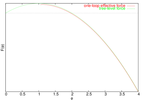
Figure 3: One-loop effective and tree-level force $F(\phi)$. The zero at the origin corresponds to the inactive state, while the zero at finite $\phi$ corresponds to an active state.

—————————————————————-

5 Discussion

In this paper we have taken the well established effective action and effective potential formalism from the quantum field theory domain and have adapted and applied it to classical field theories of the Doi and Peliti type of reacting and diffusing particles. These are field-theoretic representations of the corresponding diffusion-limited reaction problems derived from classical master equations. Apart from taking the continuum limit, the resultant actions require no further approximation and the noise is included exactly. The main result of our application is the formula for the one-loop effective potential which holds for any multiple $N$-species reaction-diffusion system subject to internal particle density fluctuations. The main goal of this paper is to illustrate the relative ease with which this effective potential can be analytically calculated in closed form and consistently renormalized for a wide variety of interesting single ($N=1$) species models, of increasing complexity, from the simplest pair annihilation case to the more intricate case of branching and annihilating random walks with arbitrary even number $m$ of offspring. We believe the most interesting specific application of the effective potential formalism in these problems is the ease with which one can deduce the associated one-loop renormalization group equations (RGE) and the effective equations of motion from it.

We have calculated the effective potential in fixed space dimension $d=2$, corresponding to the upper critical dimension for all the models surveyed here. Once the frequency integration is carried out in Eq. (3), we have seen that the remaining integral over the wavevector always reduces to the same small set of simple elementary functions (polynomials and logarithms), irrespective of the microscopic details of the specific model. This feature is what allows one to obtain potentials and the RGE’s for a wide variety of different models with little additional effort. In so far as this is a consequence of the one-loop approximation, this does represent a major technical advantage over the standard Feynman diagram approach, since in the latter approach, each individual model requires the handling of a distinct set of diagrams with its attendant combinatorics to work out. Of course, when one loop order is not sufficient, to go to higher loops, one must revert back to diagrams to compute the higher order corrections to the potential, and this can be done [18]. While individual Feynman diagrams can be analytically continued to arbitrary dimension, this appears to be more difficult for the potential, representing, as it does, an infinite summation of diagrams [22]. Nevertheless, the analytic continuation of the one-loop potential to arbitrary dimensions may be possible, and this point clearly deserves further work. This would open up the very interesting possibility to derive the associated RGE’s for a wide variety of reaction-diffusion models in a straightforward manner for any dimension $d$ in a universal way, at one-loop level, without the need to handle individual Feynman diagrams. It would be interesting to test out these analytic methods on two-species ($N=2$) reaction-diffusion systems such as the $A+B\rightarrow 0$ reaction [27]. The expression for an $N=2$ species potential requires working out the determinant of $4\times 4$ arrays, followed by integrations over frequency and wavenumber. Our conviction is that further developments of these potential methods can promote significant advances in nonequilibrium statistical mecanics and in physical chemistry. The simple examples treated here serve as a testing ground for this technique, and we believe we have amply demonstrated the usefulness of the approach and the relative ease in carrying out the specific steps leading to the renormalization group equations.

Appendix A Effective potential

In this appendix we derive the one-loop effective potential Eq. (3) for Doi-Peliti type stochastic field theories. Following standard procedures [5, 6], one starts from the microscopic master equation corresponding to the specific chemical reactions to be studied and then passes to a field-theoretic solution of this master equation. In the final step, one obtains a path integral representation of the time-evolution operator (or “hamiltonian”) of the general form

$$Z\sim\int\Pi^{N}_{j}(\mathcal{D}\psi_{j}\mathcal{D}\bar{\psi}_{j})\exp\Big{(}-S[\psi_{i},\bar{\psi}_{i}]\Big{)},$$ (124)

for ${N}$-species of particles $\psi_{i}$ and ${N}$ conjugate or “response” fields $\bar{\psi}_{i}$ for $i=(1,2,\ldots,N)$, and where $S$ denotes the unrenormalized (bare) action. Introduce the loop counting parameter $\mathcal{A}=1$ in the exponential in Eq. (124) as follows

$$S[\psi_{i},\bar{\psi}_{i}]\rightarrow S[\psi_{i},\bar{\psi}_{i}]/\mathcal{A}.$$ (125)

Fluctuations are taken into account via the loop expansion in powers of $\mathcal{A}$. Since the loop expansion corresponds to an expansion in a parameter that multiplies the entire action, it is unaffected by shifts of fields.

We next adapt the basic steps that take us from an action $S$ to the effective action and effective potential [1, 7, 18, 19, 20, 21, 22]. First, we introduce a set of arbitrary source functions $J_{i}$ and $\bar{J}_{i}$ for both the $\psi_{i}$ and $\bar{\psi}_{i}$ by adding the following term to the action

$$S[\psi_{i},\bar{\psi}_{i}]\rightarrow S[\psi_{i},\bar{\psi}_{i}]+\int d^{d}x\,\int dt\,\sum_{i=1}^{N}(J_{i}\psi_{i}+{\bar{J}}_{i}{\bar{\psi}}_{i}),$$ (126)

this linear shift leads to a source dependence in the path integral Eq. (124) which we denote by $Z[J,{\bar{J}}]$. Next, introduce the functional for connected correlation functions $W[J,{\bar{J}}]$ and its Legendre transform, the effective action $\Gamma[\phi,{\bar{\phi}}]$

$$W[J,{\bar{J}}] = \mathcal{A}\ln Z[J,{\bar{J}}],$$ (127)

$$\Gamma[\phi,{\bar{\phi}}] = -W[J,{\bar{J}}]+\int d^{d}x\,\int dt\,\sum_{i=1}^{N}(J_{i}\phi_{i}+{\bar{J}}_{i}{\bar{\phi}}_{i}),$$ (128)

where

$$\phi_{i}[J,{\bar{J}}]=\frac{\delta W[J,\bar{J}]}{\delta J_{i}},\qquad{\bar{\phi}_{i}}[J,{\bar{J}}]=\frac{\delta W[J,\bar{J}]}{\delta{\bar{J}}_{i}}.$$ (129)

The fields $\phi_{i}$ and $J_{i}$ (and $\bar{\phi}_{i}$ and $\bar{J}_{i}$) make up the Legendre transform pairs. From Eq. (124,126,127), and Eq. (129), we see that the fields $\phi_{i},\bar{\phi}_{i}$ are the fluctuation averages of the original degrees of freedom, but evaluated in the presence of the source terms, that is,

$$\phi_{i}[J,{\bar{J}}]=\langle\psi_{i}(x,t)\rangle_{J,{\bar{J}}}\qquad{\bar{\phi}}_{i}[J,{\bar{J}}]=\langle\bar{\psi}_{i}(x,t)\rangle_{J,{\bar{J}}}\,,$$ (130)

where the angular brackets denote the average over the fluctuations. These fluctuation-averaged fields are the solutions of the effective equations of motion

$$\Big{(}\frac{\delta\Gamma[\phi,\bar{\phi}]}{\delta\phi_{i}}\Big{)}\Big{|}_{\phi[J,\bar{J}],\bar{\phi}[J,\bar{J}]}=J_{i},\qquad\Big{(}\frac{\delta\Gamma[\phi,\bar{\phi}]}{\delta\bar{\phi}_{i}}\Big{)}\Big{|}_{\phi[J,\bar{J}],\bar{\phi}[J,\bar{J}]}={\bar{J}}_{i},$$ (131)

in the presence of the source terms, a fact which follows immediately from differentiating Eq. (128) as indicated. Most importantly, once we set the external sources to zero in Eq. (131), $J,\bar{J}=0$, we then obtain the effective equations of motion for the stochastic-averaged fields. The solutions are the stationary points of the effective action:

$$\Big{(}\frac{\delta\Gamma[\phi,\bar{\phi}]}{\delta\phi_{i}}\Big{)}\Big{|}_{\phi[0,0],\bar{\phi}[0,0]}=0,\qquad\Big{(}\frac{\delta\Gamma[\phi,\bar{\phi}]}{\delta\bar{\phi}_{i}}\Big{)}\Big{|}_{\phi[0,0],\bar{\phi}[0,0]}=0.$$ (132)

We make use of Eq. (132) in the paper in specific reaction diffusion models and explicitly obtain the fluctuation-modified effective equations of motion satisfied by the noise-averaged particle densities at one-loop order.

To complete the derivation of the one-loop effective potential (and suppressing writing out the full dependence on indices, and spatial and temporal arguments) we henceforth let $(\phi,\bar{\phi})$ denote the set of the source-free fluctuation averages of the $2N$ scalar fields $\{\langle\psi_{i}\rangle_{(0,0)},\langle\bar{\psi}_{i}\rangle_{(0,0)}\}_{i=1}^{N}$. Then the effective action for the field theory described by Eq. (124) is given by [20]

$$\Gamma[\phi,{\bar{\phi}}]=S[\phi,{\bar{\phi}}]+\mathcal{A}\Gamma_{1}[\phi,{\bar{\phi}}]+O(\mathcal{A}^{2}),$$ (133)

where the one-loop contribution is explicitly calculated to be

$$\Gamma_{1}[\phi,{\bar{\phi}}]=\frac{1}{2}\mathrm{Tr}[\mathrm{Ln}\,S^{(2)}(\phi,{\bar{\phi}};x,y)-\mathrm{Ln}\,S^{(2)}(0,1;x,y)],$$ (134)

and $\mathrm{Tr}$ and $\mathrm{Ln}$ are functional traces and logarithms (these operate on both discrete and continuous indices). The array $S^{(2)}$ of second order functional derivatives of the action with respect to the fields is expressed in $2\times 2$ block array form in Eq. (1), where $i,j=(1,2,\ldots,N)$. The action $S[\phi,{\bar{\phi}}]$ is simply the action Eq. (125) after replacing $\psi_{i}$ and $\bar{\psi}_{i}$ by $\phi_{i}$ and $\bar{\phi}_{i}$, respectively. The effective potential is the effective action Eq. (133) evaluated on constant field configurations, and after dividing out by the overall volume of space-time $VT$:

$$\mathcal{V}[\phi,{\bar{\phi}}]\equiv\frac{\Gamma[\phi,{\bar{\phi}}]}{VT} = \frac{S[\phi,{\bar{\phi}}]}{VT}+\mathcal{A}\frac{\Gamma_{1}[\phi,{\bar{\phi}}]}{VT}+O(\mathcal{A}^{2})$$ (135)

$$= V_{0}[\phi,{\bar{\phi}}]+\mathcal{A}V_{1}[\phi,{\bar{\phi}}]+O(\mathcal{A}^{2}).$$

For constant fields $\phi,{\bar{\phi}}=\textrm{const.}$, we pass to Fourier space and define a $2N\times 2N$ matrix $M$ via the Fourier transform (FT) of Eq. (1) as defined in Eq. (2). Since this expression is diagonal in momentum and frequency, we can straightforwardly carry out the sequence of operations indicated in Eq. (134) [18]:

$$\mathrm{Tr}\mathrm{Ln}[M(k,\omega;\phi,{\bar{\phi}})\times(2\pi)^{d+1}\delta^{d}(k-p)\delta(\omega-\Omega)]$$ (136)

$$= \mathrm{Tr}(2\pi)^{d+1}\delta^{d}(k-p)\delta(\omega-\Omega)\ln M(k,\omega,\phi,\bar{\phi})$$

$$= \int\frac{d^{d}k}{(2\pi)^{d}}\int\frac{d\omega}{2\pi}(2\pi)^{d+1}\delta^{d}(k-p)\delta(\omega-\Omega)|_{k=p,\omega=\Omega}\,\mathrm{tr}\ln M(k,\omega,\phi,\bar{\phi})$$

$$= \int d^{d}x\,\int dt\,\int\frac{d^{d}k}{(2\pi)^{d}}\int\frac{d\omega}{2\pi}\ln\det M(k,\omega,\phi,\bar{\phi}),$$

where $\ln$ and $\mathrm{tr}$ are the ordinary logarithm and trace, and we have used the identity $\mathrm{tr}\ln M=\ln\det M$. Evaluating Eq. (133) on constant configurations and dividing through by the volume of space-time and using Eq. (1,2,134,135) and Eq. (136), yields the compact expression for the one-loop effective potential Eq. (3).

Acknowledgements
M.-P.Z. acknowledges a fellowship provided by INTA for training in astrobiology. The research of D.H. is supported in part by funds from CSIC and INTA.

References

- [1] D. Hochberg, C. Molina-París, J. Pérez-Mercader and M. Visser, Effective action for stochastic partial differential equations, Phys. Rev. E 60:6343-6360 (1999).
- [2] K. Oerding, F. van Wijland, J.-P. Leroy and H.J. Hilhorst, Fluctuation-Induced First-Order Transition in a Nonequilibrium Steady State, J. Stat. Phys. 99:1365-1395 (2000).
- [3] H.K. Janssen, Ü. Kutbay and K. Oerding, Equation of state for directed percolation, J. Phys. A: Math. Gen. 32:1809-1817 (1999).
- [4] L. Canet, B. Delamotte, O. Deloubrière and N. Wschebor, Nonperturbative Renormalization-Group Study of Reaction-Diffusion Processes , Phys. Rev. Lett. 92:195703(1)-195703(4) (2004); L. Canet, H. Chaté and B. Delamotte, Quantitative Phase Diagrams of Branching and Annihilating Random Walks, Phys. Rev. Lett. 92:255703(1)-255703(4) (2004).
- [5] M. Doi, Second quantization representation for classical many-particle system, J. Phys. A: Math. Gen. 9:1465-1477 (1976).
- [6] L. Peliti, Path integral approach to birth-death processes on a lattice, J. Physique 46:1469-1483 (1985).
- [7] D. Hochberg, J. Pérez-Mercader, C. Molina-París and M. Visser, Renormalization Group Improving the Effective Action: A Review, Int. J. Mod. Phys. A 14: 1485-1521 (1999).
- [8] Y. Fujimoto, L. O’Raifeartaigh and G. Parravicini, Effective potential for non-convex potentials, Nucl. Phys. B212:268-300 (1983).
- [9] B. Gato, J. Leon, J. Pérez-Mercader and M. Quirós, Renormalization group analysis for a general softly broken supersymmetric gauge theory, Nucl. Phys. B253:285-307 (1985).
- [10] D. Toussaint and F. Wilczek, Particle-antiparticle annihilation in diffusive motion, J. Chem. Phys. 78:2642-2647 (1983).
- [11] K. Kang and S. Redner, Scaling approach for the Kinetics of Recombination Processes, Phys. Rev. Lett. 52:955-958 (1984).
- [12] L. Peliti, Renormalisation of fluctuation effects in the reaction, J. Phys. A: Math. Gen. 19:L365-L367 (1986).
- [13] T. Ohtsuki, Field-theoretical aproach to scaling behavior of diffusion-controlled recombination, Phys. Rev. A43: 6917-6919 (1991).
- [14] M. Droz and L. Sasvári, Renormalization-group approach to simple reaction-diffusion phenomena, Phys. Rev. E48:R2343-R2346 (1993).
- [15] B. Friedman, G. Levine and B. O’Shaughnessy, Renormalization-group study of field-theoretic , Phys. Rev. A46: R7343-R7346 (1992).
- [16] B.P. Lee, Renormalization group calculation for the reaction , J. Phys. A: Math Gen. 27:2633-2652 (1994).
- [17] I.S. Gradshteyn and I.M. Ryzhik, Table of Integrals, Series and Products (Academic Press, New York, 1980).
- [18] R. Jackiw, Functional evaluation of the effective potential, Phys. Rev. D9:1686-1701 (1974).
- [19] J. Iliopoulos, C. Itzykson, A. Martin, Functional methods and perturbation theory, Rev. Mod. Phys. 47:165-192 (1975).
- [20] J. Zinn-Justin, Quantum Field Theory and Critical Phenomena (Oxford University Press, Oxford, 2002) 4rth edition.
- [21] R.J. Rivers, Path integral methods in quantum field theory (Cambridge University Press, Cambridge, 1988).
- [22] S. Coleman and E. Weinberg, Radiative Corrections as the Origin of Spontaneous Symmetry Breaking, Phys. Rev. D7:1888-1910 (1973).
- [23] P. Grassberger and K. Sundermeyer, Reggeon field theory and Markov processes, Phys. Lett. 77B:220-222 (1978).
- [24] H.K. Janssen, On the Nonequilibrium Phase Transition in Reaction-Diffusion Systems with an Absorbing Stationary State, Z. Phys. B42:151-154 (1981).
- [25] M.J. Howard and U.C. Täuber, Real versus imaginary noise in diffusion-limited reactions, J. Phys. A: Math. Gen. 30:7721-7731 (1997).
- [26] J.L. Cardy and U.C. Täuber, Field Theory of Branching and Annihilating Random Walks, J. Stat. Phys. 90:1-56 (1998).
- [27] B.P. Lee and J. Cardy, Renormalization Group Study of the Diffusion-Limited Reaction, J. Stat. Phys. 80:971-1007 (1995); ibid. 87:951-954 (1997).