Giant Magneto-Oscillations of Electric-Field-Induced Spin Polarization in 2DEG

Abstract

We consider a disordered two-dimensional electron gas with spin-orbit coupling placed in a perpendicular magnetic field and calculate the magnitude and direction of the electric–field–induced spin polarization. We find that in strong magnetic fields the polarization becomes an oscillatory function of the magnetic field and that the amplitude of these oscillations is parametrically larger than the polarization at zero magnetic field. We show that the enhanced amplitude of the polarization is a consequence of strong electron–hole asymmetry in a quantizing magnetic field.

I Introduction

One of the main objectives of spintronics spintron ; ZFS is to develop devices, which would control electron spins by electric fields. A potential implementation of these devices is based on the magneto-electric effect LNE ; ALG1 ; ILGP in a two-dimensional electron gas (2DEG) with spin-orbit (SO) coupling. The spin polarization of 2DEG by dc electric field, one of the manifestations of the magneto-electric effect, has recently become a focus of theoretical ALG1 ; Bc2DEG ; MSH04 ; CEM02 ; IBM03 ; TDS and experimental silov ; KatoMagn04 investigation. Despite extensive research ALG1 ; ILGP ; MSH04 ; CEM02 ; IBM03 ; Bc2DEG ; TDS ; silov ; KatoMagn04 , the electron–hole asymmetry as the cause of the magneto–electric effect has not been emphasized.

In this paper, we demonstrate that the magneto–electric effect in 2DEG is the consequence of electron–hole asymmetry. Following this observation, we explore potential mechanisms for enhancement of the electron–hole asymmetry. We find that the quantization of electron orbital motion in a perpendicular magnetic field is one of these mechanisms. Particularly, in strong magnetic field $B$ the polarization induced by an in-plane electric field oscillates as a function of $B$ with the amplitude of oscillations larger than the smooth component of the polarization by a huge factor $\nu=E_{\rm F}/\omega_{\rm c}\gg 1$, where $E_{\rm F}=p_{\rm F}^{2}/2m^{*}$ is the Fermi energy, $\omega_{\rm c}=eB/m^{*}c$ is the cyclotron frequency, $p_{\rm F}$ is the Fermi momentum, $e$ and $m^{*}$ are the charge and effective mass of electrons, $c$ is the speed of light, $\hbar=1$.

The large parameter $E_{\rm F}/\omega_{\rm c}$ is indeed related to the enhancement of electron–hole asymmetry by magnetic field. At zero magnetic field, electron scattering rate off disordered potential is nearly independent of energy. In this case the polarization is generated by electron–hole asymmetry, which is due to the curvature of the electron spectrum and is characterized by energy $E_{\rm F}$. The cyclotron motion of electrons in a perpendicular magnetic field $B$ results in quantum interference corrections to the scattering rate off disorder Ando ; VA03 . These corrections, periodic in energy, violate the electron–hole asymmetry on much smaller energy scale $\omega_{\rm c}\ll E_{\rm F}$. We note that some transport coefficients, such as the thermoelectric power 2DEGTP and the Coulomb drag transconductance GMO , can be similarly enhanced by magnetic fields.

We derive the quantum kinetic equation for a disordered 2DEG with SO coupling following the formalism developed in Ref. VA03 for 2DEG without SO coupling. We solve this equation and calculate the spin polarization for a system brought out of equilibrium by a dc in-plane electric field. The polarization can be represented as a sum of the smooth and oscillating components, as illustrated in Fig. 1. At weak magnetic fields, the oscillatory component is exponentially small, and only the smooth component remains. However, the amplitude of oscillatory component increases as magnetic field increases and becomes significantly larger than the smooth component.

The observation of the polarization oscillations induced by an electric field seems to be feasible. Indeed, recently, the non-equilibrium spin polarization in zero magnetic field was observed in experimentally KatoMagn04 ; silov , and the possibility of polarization measurements in strong magnetic fields was demonstrated in Ref. Sih .

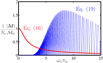
Figure 1: (Color online) The magnitude of the polarization vector is shown as a function of the magnetic field $B\propto\omega_{\rm c}$ at fixed electric field. The thick smooth line represents the result of Eq. (16) for $\lambda_{x}=\lambda_{y}$ and $g=0$. The thin line describes the oscillatory part of the polarization Eq. (19) for $\tau_{\rm tr}/\tau_{\rm q}=10$, $T=0$, $E_{\rm F}\tau_{\rm tr}=1.25\times 10^{3}$ (period of oscillations is not shown to scale).

II Qualitative Discussion

In this section we present a qualitative picture of generation of spin polarization by in-plane electric field. We show that in weak magnetic fields, when the electron DoS is energy independent, the polarization originates due to the dependence of SO coupling strength on the momentum of electron and hole excitations. On the other hand, in strong magnetic fields the DoS oscillates as a function of energy, and therefore the polarization may appear due to the difference in the number of electron and the number of hole excitations. We show that the latter mechanism may result in larger values of the spin polarization.

In equilibrium, electrons occupy all quantum states inside the Fermi surface, which for 2DEG is a circle in momentum space, centered at $\bm{p}=0$ and shown by a solid line in Fig. 2a. However, if an electric field is applied and finite current $\bm{j}$ flows in the system, the electron distribution is shifted in momentum space by vector $\Delta\bm{p}\simeq p_{\rm F}(\bm{j}/j_{\rm F})$, where $j_{\rm F}=ev_{\rm F}N_{\rm e}$ and $N_{\rm e}=p_{\rm F}^{2}/2\pi$ is the sheet density of 2DEG. In this case electrons occupy all states within the dashed circle in Fig. 2a, centered at $\bm{p}=\Delta\bm{p}$. The depleted states are called hole excitations (holes) and the newly occupied states are called electron excitations (electrons).

The net spin polarization $\bar{M}$ of 2DEG is determined by the sum of the electron and hole polarizations. Since these two polarizations are directed in opposite directions, they mostly compensate each other. However, for the linear in momentum SO coupling $\hat{H}=\bm{p}\times\hat{\bm{\sigma}}/m^{*}\lambda_{\rm so}$, the strength of the SO coupling is stronger for electron excitations than for hole excitations, as illustrated in Fig. 2a. As the result, the magnitude of the spin polarization due to the SO coupling of electrons a little bit exceeds that of holes. The net polarization can be estimated as the difference in the energy $\Delta E\simeq|\Delta\bm{p}|/m^{*}\lambda_{\rm so}$ of spin states of electron and hole excitations, multiplied by the DoS $\nu_{0}=m^{*}/2\pi$. We find

$$\frac{\bar{M}}{N_{\rm e}}\simeq\frac{|\Delta\bm{p}|}{m^{*}\lambda_{\rm so}}\frac{\nu_{0}}{N_{\rm e}}\simeq\frac{E_{\rm so}}{E_{\rm F}}\frac{j}{j_{\rm F}},$$ (1)

where $E_{\rm so}=v_{\rm F}/\lambda_{\rm so}$. From Fig. 2a we can also conclude that the vector of the spin polarization is perpendicular to $\bm{j}$.

We note that the polarization is determined by the actual current density $\bm{j}=\sigma_{\rm D}\check{R}(\omega_{\rm c}\tau_{\rm tr})\bm{E}$ linear in the electric field $\bm{E}$, where

$$\sigma_{\rm D}=\frac{e^{2}\nu_{0}v_{\rm F}^{2}\tau_{\rm tr}}{2},\quad\check{R}(x)=\frac{1}{x^{2}+1}\left[\begin{array}[]{cc}1&-x\\ x&1\\ \end{array}\right]$$ (2)

is the Drude conductivity tensor in the magnetic field $B\propto\omega_{\rm c}$ and $\tau_{\rm tr}$ is the transport scattering time. Consequently, if the current density $\bm{j}$ is fixed, the polarization is independent of magnetic field. However, if the electric field $\bm{E}$ is fixed in the sample, then, according to Eqs. (1) and (2), the polarization decreases and changes its orientation as the magnetic field increases.

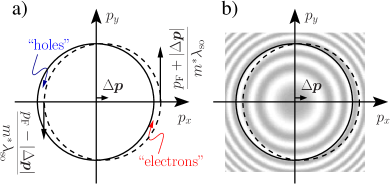
Figure 2: (Color online) a) In equilibrium, electrons occupy all states within Fermi surface – a solid circle centered at $\bm{p}=0$. When electric field is applied, electrons occupy all states within the dashed circle, centered at $\Delta\bm{p}\propto\bm{j}$. States that become empty are called hole excitations and states that become occupied are called electron excitations. The numbers of electron and hole excitations are equal, and the spin polarization occurs only due to the difference in the SO coupling of electrons and holes, see Eq. (1). The latter is stronger for electrons, that have larger momentum, than for holes with smaller momentum. b) In magnetic field, the DoS is modulated, as shown here by a contour plot. The numbers of electron and hole excitations are different and the spin polarization can be obtained even when the difference in SO coupling for electron and hole excitations is neglected.

When the magnetic field becomes strong enough and $\omega_{\rm c}\tau_{\rm q}\gtrsim 1$, the electron DoS oscillates as a function of energy, where $\tau_{\rm q}$ is the quantum scattering time. As we discussed above, if a finite current flows in 2DEG, the electron distribution is shifted in momentum space. Now, due to the oscillations of the DoS, see Fig. 2b, the number of electrons and the number of holes may be different. In this case we can neglect the dependence of SO coupling on the magnitude of the excitations’ momentum and estimate the spin polarization $\tilde{M}$ as the difference in the DoS of electron and hole excitations, multiplied by the energy of SO splitting $E_{\rm so}$, we have $\tilde{M}\simeq\delta\nu E_{\rm so}$. If electron density of states oscillates with period $\omega_{\rm c}$, we write $\Delta\nu\propto\nu_{0}v_{\rm F}|\Delta p|/\omega_{\rm c}$ and obtain

$$\frac{\tilde{M}}{N_{\rm e}}\propto\frac{E_{\rm so}}{\omega_{\rm c}}\frac{j}{j_{\rm F}}.$$ (3)

Comparing Eqs. (1) and (3), we conclude that the spin polarization due to the oscillations in the DoS contains the large factor $E_{\rm F}/\omega_{\rm c}\gg 1$, and therefore may be significantly larger than the polarization at zero magnetic field.

In the above discussion we assumed that electron temperature is zero. Temperature smearing of electron distribution function does not affect the result of Eq. (1), calculated for the constant DoS, but the estimate Eq. (3) for oscillating DoS would contain difference of the DoS of electron and hole excitations, averaged over the thermally smeared part of the distribution function. This difference is suppressed if temperature is higher than the period $\omega_{\rm c}$ of oscillations of the DoS. Thus, Eq. (3) represents the upper limit for the spin polarization in strong magnetic fields and the actual polarization may be smaller. In the rest of this paper we present the results of detailed analytical calculations of the spin polarization in weak and strong magnetic fields.

III Kinetic equation

We consider a 2DEG with linear in momentum SO coupling, placed in a perpendicular magnetic field, when the filling factor $\nu=E_{\rm F}/\omega_{\rm c}\gg 1$. In this case we can use the quantum kinetic theory VA03 developed within the self-consistent Born approximation Ando . We assume that the correlation length of disorder $\xi$ is much longer than the Fermi wavelength $\lambda_{\rm F}=2\pi/p_{\rm F}$, and therefore the ratio of the transport scattering time $\tau_{\rm tr}$ to the quantum scattering time $\tau_{\rm q}$ is large, $\tau_{\rm tr}/\tau_{\rm q}\sim(\xi p_{\rm F})^{2}\gg 1$. The kinetic equation has the form:

$$\partial_{t}\hat{f}(t,\varepsilon)+i[\hat{H};\hat{f}(t,\varepsilon)]={\rm St}\{\hat{f}(t,\varepsilon)\},$$ (4)

where $[\hat{A};\hat{B}]=\hat{A}\hat{B}-\hat{B}\hat{A}$ and

$$\hat{H}=\frac{\hat{\bm{P}}^{2}}{2m^{*}}+e\bm{E}\bm{r}-\frac{\Delta_{g}}{2}\hat{\sigma}_{z},\ \Delta_{g}=g\mu_{\rm B}B$$ (5)

is the Hamiltonian of 2DEG in a quantum well with

$$\hat{\bm{P}}=\bm{p}+\hat{\bm{\Lambda}};\quad\hat{\Lambda}_{x}=\frac{\hat{\sigma}_{y}}{\lambda_{x}},\ \hat{\Lambda}_{y}=-\frac{\hat{\sigma}_{x}}{\lambda_{y}}.$$ (6)

Here $\bm{p}$ is the momentum operator and $\hat{\bm{\Lambda}}$ characterizes the SO coupling and contains both the Rashba (the only term if $\lambda_{x}=\lambda_{y}$) and crystalline anisotropy terms. The second term in Eq. (5) describes the effect of the in-plane electric field $\bm{E}$, and the last term represents the Zeeman energy, $g$ is the electron gyromagnetic factor, $\mu_{\rm B}=e/(2m_{\rm e}c)$ is the Bohr magneton, $m_{\rm e}$ is the free-electron mass.

In smooth disorder, the collision integral in Eq. (4) can be represented in the form, see Ref. VA03 :

$${\rm St}\{\hat{f}(\varepsilon)\}=\frac{\nabla_{\hat{\bm{P}}}^{2}\{\hat{\nu}(\varepsilon);\hat{f}(\varepsilon))\}-\{\nabla_{\hat{\bm{P}}}^{2}\hat{\nu}(\varepsilon);\hat{f}(\varepsilon)\}}{2\nu_{0}\tau_{\rm tr}}.$$ (7)

Here $\nabla_{\hat{\bm{P}}}=\hat{\bm{P}}\times\partial_{\hat{\bm{P}}}$, $\{\hat{A};\hat{B}\}=\hat{A}\hat{B}+\hat{B}\hat{A}$, and $\nu_{0}=m^{*}/(2\pi)$ is DOS per spin in zero magnetic field. We neglected the Zeeman term in Eq. (7). This approximation is justified in weak magnetic fields, when the Zeeman energy is small, as well as in strong magnetic fields, when the spin orientation is fixed by the Zeeman field and $\nabla_{\hat{\bm{P}}}$ can be replaced by $\nabla_{\bm{p}}$. Note that the collision integral is determined by the electron DoS $\hat{\nu}(\varepsilon)$ VA03 .

In a perpendicular magnetic field $B$, the momentum operators $p_{\alpha}$ ($\alpha=x,y$) do not commute:

$$[p_{\alpha};p_{\beta}]=-\frac{i}{\lambda_{H}^{2}}\epsilon_{\alpha\beta};\ \ \ \check{\epsilon}=\left[\begin{array}[]{cc}0&1\\ -1&0\\ \end{array}\right];\ \ \ \lambda_{H}=\sqrt{\frac{c}{eB}}.$$ (8)

We represent the momentum operator $\bm{p}$ in the form

$$\bm{p}=p_{\rm F}\mbox{\boldmath$i$}_{\varphi}+\delta\bm{p},\quad\delta\bm{p}=\frac{1}{2R_{\rm c}}\left\{\begin{array}[]{c}ne^{i\varphi}+e^{-i\varphi}n\\ -ine^{i\varphi}+ie^{-i\varphi}n\\ \end{array}\right\},$$ (9)

where $\mbox{\boldmath$i$}_{\varphi}=(\cos\varphi,\sin\varphi)$ and $R_{\rm c}=v_{\rm F}/\omega_{\rm c}$ is the cyclotron radius. To satisfy Eq. (8), the operators $n$ and $\varphi$ have to obey the following commutation relation

$$[n;e^{i\varphi}]=e^{i\varphi};\quad n\to-i\partial_{\varphi}.$$ (10)

The integer eigenvalues of the operator $n$ have the meaning of the Landau level indices.

In the representation (9) of momentum operators $\bm{p}$, we have $\hat{\bm{P}}^{2}/2m^{*}=\omega_{\rm c}n+v_{\rm F}\mbox{\boldmath$i$}_{\varphi}\hat{\bm{\Lambda}}+\hat{H}_{\rm sc}$, where $\hat{H}_{\rm sc}=\delta\bm{p}\hat{\bm{\Lambda}}/m^{*}$ describes the asymmetry of the SO coupling between electron and hole excitations, discussed in the previous Section and illustrated in Fig. 2a. Below we show that only the term $\hat{H}_{\rm sc}$ couples the spin and charge components of the electron distribution function in weak (non-quantizing) magnetic fields. We further simplify the kinetic equation by performing an auxiliary transformation $\hat{\cal U}_{\delta}=\exp\{i\lambda_{H}^{2}(\delta\mbox{\boldmath$p$}\check{\epsilon}\hat{\bm{\Lambda}})\}$ of $\hat{\bm{P}}^{2}/2m^{*}$, and keeping terms up to the second order in $\delta\mbox{\boldmath$p$}\check{\epsilon}\hat{\bm{\Lambda}}$. This transformation is an analogue of the unitary transformation of the Hamiltonian in zero magnetic field fn1 and corresponds to a tiny rotation of the momentum and spin states on “angle” $\lambda_{H}^{2}(\delta\mbox{\boldmath$p$}\check{\epsilon}\hat{\bm{\Lambda}})\sim\lambda_{\rm F}/\lambda_{x,y}\ll 1$. Therefore, we neglect the transformation under $\hat{\cal U}_{\delta}$ of the electron distribution function, $\hat{f}$; the spin operator, $\hat{\bm{\sigma}}$; and the Zeeman energy term. This transformation is used only to simplify $\nabla_{\hat{\bm{P}}}$ in the collision integral and $\hat{H}_{\rm sc}$, the latter in the new basis is

$$\hat{H}_{\rm sc}=\frac{\hat{\sigma}_{z}}{m^{*}\lambda_{x}\lambda_{y}}\left(-2i\partial_{\varphi}+1\right).$$ (11)

The spin-charge coupling, $\hat{H}_{\rm sc}$, originates from the electron-hole asymmetry of the Hamiltonian Eq. (5) (due to the difference in velocities of electrons and holes at distance $\delta\bm{p}$ from the Fermi surface). The factor $1/(m^{*}\lambda_{x}\lambda_{y})$ can be associated with the curvature of electron energy bands in momentum space (cf. Refs. Bc ; Bc2DEG , where the effect of the Berry curvature on motion in coordinate space is considered). The above derivation of Eq. (11) was based on the representation Eq. (9), defined at $B\neq 0$; the same form $\hat{H}_{\rm sc}$ is valid at $B=0$ ALG04 .

For a spatially homogeneous and stationary in time system, to the lowest order in $\lambda_{\rm F}/\lambda_{x,y}$, we obtain the following kinetic equation:

$$\begin{split}\partial_{t}\hat{f}+&\omega_{\rm c}\partial_{\varphi}\hat{f}+i\left[v_{\rm F}\mbox{\boldmath$i$}_{\varphi}\hat{\bm{\Lambda}}-\frac{\Delta_{g}}{2}\hat{\sigma}_{z};\hat{f}\right]\\ &+i[\hat{H}_{\rm sc};\hat{f}]+ev_{\rm F}\mbox{\boldmath$i$}_{\varphi}\bm{E}\partial_{\varepsilon}\hat{f}=\frac{\{\hat{\nu}(\varepsilon);\partial_{\varphi}^{2}\hat{f}\}}{2\nu_{0}\tau_{\rm tr}},\end{split}$$ (12)

where function $\hat{f}(\varepsilon,\varphi)$ describes the distribution of electrons with momentum $p$ in the direction $\mbox{\boldmath$i$}_{\varphi}$. The second term $i\omega_{\rm c}[n;\hat{f}]=\omega_{\rm c}\partial_{\varphi}\hat{f}$ in the left hand side of Eq. (12) describes the Lorentz force acting on electrons in magnetic field $B\propto\omega_{\rm c}$. The fourth term $i[\hat{H}_{\rm sc};\hat{f}]$ with $\hat{H}_{\rm sc}$ given by Eq. (11) has a similar structure and can be associated with the Lorentz force, induced by the SO coupling. Below we solve Eq. (12) in the limits of weak ($\omega_{\rm c}\tau_{\rm q}\lesssim 1$) and strong ($\omega_{\rm c}\tau_{\rm q}\gtrsim 1$) magnetic fields.

IV Weak magnetic field

At $\omega_{\rm c}\tau_{\rm q}\ll 1$, the oscillatory component of the DOS $\hat{\nu}(\varepsilon)$ is exponentially suppressed and $\hat{\nu}(\varepsilon)=\hat{1}\nu_{0}$. We solve the kinetic equation Eq. (12) by consecutive iterations, limiting our consideration to the limit of weak SO coupling, $\lambda_{x,y}\gg v_{\rm F}\tau_{\rm tr}$. We start with the Fermi distribution function $\hat{f}(\varepsilon)=\hat{1}f_{\rm F}(\varepsilon)$, $f_{\rm F}(\varepsilon)=(\exp((\varepsilon-E_{\rm F})/T)+1)^{-1}$. To first order in the electric field $\bm{E}$ the distribution function contains an anisotropic component with respect to the momentum direction $\varphi$:

$$\hat{f}^{(1)}(\varepsilon,\varphi)=-\hat{1}\frac{2\sigma_{\rm D}}{ev_{\rm F}\nu_{0}}\left(\mbox{\boldmath$i$}_{\varphi}^{T}\check{R}(\omega_{\rm c}\tau_{\rm tr})\bm{E}\right)f^{\prime}_{\rm F}(\varepsilon),$$ (13)

where $\sigma_{\rm D}\check{R}(\omega_{\rm c}\tau_{\rm tr})$ is the Drude conductivity matrix Eq. (2).

The distribution function $\hat{f}^{(1)}(\varepsilon,\varphi)$ has no spin components. The spin components in $\hat{f}$ appear only if the spin-charge coupling term $i[\hat{H}_{\rm sc};\hat{f}]$ is taken into account in Eq. (12). Keeping $i[\hat{H}_{\rm sc};\hat{f}^{(1)}(\varepsilon,\varphi)]$ with $\hat{H}_{\rm sc}$ and $\hat{f}^{(1)}(\varepsilon,\varphi)$ given by Eqs. (11) and (13), we obtain the solution of Eq. (12) after the second iteration in the form:

$$\hat{f}^{(2)}(\varepsilon,\varphi)=-\hat{\sigma}_{z}\frac{4\sigma_{\rm D}\tau_{\rm tr}}{ev_{\rm F}\nu_{0}}\frac{[\mbox{\boldmath$i$}_{\varphi}^{T}\check{\epsilon}\check{R}^{2}(\omega_{\rm c}\tau_{\rm tr})\bm{E}]}{m^{*}\lambda_{x}\lambda_{y}}f^{\prime}_{\rm F}(\varepsilon).$$ (14)

Still, $\hat{f}^{(2)}(\varepsilon,\varphi)$ does not describe spin polarization of 2DEG because $\int d\varphi\hat{f}^{(2)}(\varepsilon,\varphi)=0$. Substituting $\hat{f}^{(2)}(\varepsilon,\varphi)$ into the second term in the left hand side (LHS) of Eq. (12), we look for a solution $\hat{f}^{(3)}(\varepsilon,\varphi)=\bm{f}^{(3)}(\varepsilon)\bm{\sigma}+\bm{\alpha}(\varepsilon)\mbox{\boldmath$i$}_{\varphi}\hat{\sigma}_{z}$. Here $\bm{f}^{(3)}(\varepsilon)\bm{\sigma}=\sum_{j=x,y}f_{j}\hat{\sigma}_{j}$ is an isotropic spin term, which determines the polarization of 2DEG. First, we express $\bm{\alpha}(\varepsilon)\mbox{\boldmath$i$}_{\varphi}$ in terms of $\bm{f}^{(3)}(\varepsilon)$, then, we insert $\bm{\alpha}(\varepsilon)\mbox{\boldmath$i$}_{\varphi}$ into the second term in LHS of Eq. (12) and average the result over $\mbox{\boldmath$i$}_{\varphi}$. This procedure is equivalent to neglecting higher harmonics in $\mbox{\boldmath$i$}_{\varphi}$, small in the parameter $v_{\rm F}\tau_{\rm tr}/\lambda_{x,y}\ll 1$. We find

$$\begin{split}&\bm{f}^{(3)}(\varepsilon)=\kappa\check{K}(\omega_{\rm c}\tau_{\rm tr})\bm{g},\ \ \ \kappa=\frac{\lambda_{x}\lambda_{y}}{2v_{\rm F}^{2}\tau_{\rm tr}},\\ &\hat{K}(x)=\frac{\displaystyle\left[\begin{array}[]{cc}\lambda_{x}/\lambda_{y}&x(1+\eta(1+x^{2}))\\ -x(1+\eta(1+x^{2}))&\lambda_{y}/\lambda_{x}\\ \end{array}\right]}{(x^{2}(1+\eta(1+x^{2}))^{2}+1)(1+x^{2})^{-1}}.\end{split}$$ (15)

The vector $\bm{g}$ is the spin generation matrix $\bm{g}\hat{\bm{\sigma}}=iv_{\rm F}\int\mbox{\boldmath$i$}_{\varphi}[\hat{\bm{\Lambda}};\hat{f}^{(2)}(\varepsilon,\varphi)]d\varphi/2\pi$, the matrix $(\kappa\check{K})^{-1}$ is the spin relaxation matrix, and $\eta=g(m/m_{\rm e})(\lambda_{x}\lambda_{y}/4v_{\rm F}^{2}\tau_{\rm tr}^{2})$ characterizes the strength of the Zeeman splitting.

The ratio of spin density $\bm{M}=\nu_{0}\int\bm{f}^{(3)}(\varepsilon)d\varepsilon$ to the total electron density $N_{\rm e}=p_{\rm F}^{2}/2\pi$ of 2DEG is

$$\begin{split}\frac{\bm{M}}{N_{\rm e}}&={\cal M}_{0}\bm{m},\quad{\cal M}_{0}=\frac{\lambda_{\rm F}^{2}}{(2\pi)^{2}}\frac{e|\bm{E}|\tau_{\rm tr}}{\sqrt{\lambda_{x}\lambda_{y}}},\\ \bm{m}&=\check{K}\check{L}\check{\epsilon}\check{R}^{2}(\omega_{\rm c}\tau_{\rm tr})\bm{e},\quad\check{L}=\left[\begin{array}[]{cc}\sqrt{\frac{\lambda_{y}}{\lambda_{x}}}&0\\ 0&\sqrt{\frac{\lambda_{x}}{\lambda_{y}}}\\ \end{array}\right],\end{split}$$ (16)

where $\lambda_{\rm F}=2\pi/p_{\rm F}$ is the Fermi wavelength, length scales $\lambda_{x,y}$ describe the strength of the SO coupling, Eq. (6), and matrices $\hat{R}$ and $\hat{K}$ are introduced in Eqs. (2) and (15).

The direction of the spin polarization $\bm{M}$ is given by the vector $\bm{m}$, which is related to the direction of the electric field $\bm{e}=\bm{E}/|\bm{E}|$ through the tensor $\check{K}\check{L}\check{\epsilon}\check{R}^{2}$. For the Rashba coupling, $\lambda_{\rm so}=\lambda_{x,y}$, Eq. (16) coincides with the result of Ref. ALG1 ; MSH04 at $B=0$, obtained for point-like scatters, if the full scattering time is replaced by $\tau_{\rm tr}$. We can reduce Eq. (16) in case $\eta\propto g=0$ and $\lambda_{\rm so}=\lambda_{x,y}$ to $\bm{M}/N_{\rm e}=(E_{\rm so}/E_{\rm F})(\check{\epsilon}\bm{j}/j_{\rm F})$, where $\bm{j}=\sigma_{\rm D}\check{R}(\omega_{\rm c}\tau_{\rm tr})\bm{E}$ is the electric current density, $E_{\rm so}=v_{\rm F}/\lambda_{\rm so}$ is the SO energy splitting, and $j_{\rm F}=ev_{\rm F}N_{\rm e}$ (the current density if all electrons were moving with velocity $v_{\rm F}$). In typical 2DEG, $E_{\rm so}\ll E_{\rm F}$ and $|\bm{j}|\ll j_{\rm F}$, thus the polarization is small: $|\bm{M}|/N_{\rm e}\ll 1$. Note that for fixed $\bm{j}$, $\bm{m}$ is independent of $B$. Finite $g$ factor and anisotropy of SO coupling ($\lambda_{x}\neq\lambda_{y}$) do not significantly change the value of $|\bm{M}|/N_{\rm e}$, but result in more complicated behavior of $\bm{m}$ as a function of $B$. For fixed $\bm{E}$, we show dependence of $|\bm{m}|$ on $B\propto\omega_{\rm c}$ in Fig. 1 and the parametric plot of $\bm{m}(B)$ in $(m_{x},m_{y})$ plane in Fig. 3.

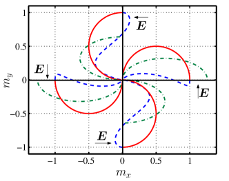
Figure 3: (Color online) A parametric dependence of the polarization vector on the orbital magnetic field $B\propto\omega_{\rm c}\tau_{\rm tr}$ is shown for different values of $\eta$ and $\lambda_{x}/\lambda_{y}$. The curves represent the Rashba coupling ($\lambda_{x}=\lambda_{y}$) with $\eta=0$ [solid line] and $\eta=1$ [dashed line]. The dash-dotted line represents $\lambda_{x}=2\lambda_{y}$ and $g=0$.

V Strong Magnetic field

As the magnetic field increases, the polarization Eq. (16) decreases. However, if $\omega_{\rm c}\tau_{\rm q}\gtrsim 1$, DOS becomes an oscillating function of energy shifted in opposite directions for different spin states. The magnitude of the shift is equal to either the Zeeman energy $\Delta_{g}$, Eq. (5), or the SO energy $\Delta_{\lambda}$, see Eq. (20) below.

We first discuss the case of strong magnetic fields $B\gtrsim B_{*}$, when $\Delta_{g}\gg\Delta_{\lambda}$, $B_{*}=(c/e)\sqrt{m_{\rm e}/gm^{*}}/\lambda_{x,y}\lambda_{\rm F}$ and the splitting of the spin states is dominated by the Zeeman effect. In strong magnetic fields we can neglect the effect of the SO coupling on the electron DoS. In this case we can obtain the DoS for the two spin projections $\sigma_{z}/2$ on magnetic field independently from each other following the derivation in Ref. VA03 and taking into account the Zeeman splitting $\Delta_{g}=g\mu_{\rm B}B$:

$$\nu_{\sigma_{z}}=\nu_{0}\left[1+2\sum_{l=1}^{\infty}(-\delta)^{l}g_{l}\cos\frac{2\pi l(\varepsilon-\sigma_{z}\Delta_{g}/2)}{\omega_{\rm c}}\right],$$ (17)

where the spectral coefficients $g_{l}=L_{l-1}^{1}(2\pi l/\omega_{\rm c}\tau_{\rm q})/l$ are expressed in terms of the Laguerre polynomials $L_{n}^{m}(x)$, and $\delta=\exp(-\pi/\omega_{\rm c}\tau_{\rm q})$.

The electric field $\bm{E}$ generates an anisotropic component of the electron distribution function: $\hat{f}^{(1)}(\varepsilon,\varphi)=\hat{1}f^{(1)}_{\rm c}(\varepsilon,\varphi)+\hat{f}^{(1)}_{\rm s}(\varepsilon,\varphi)$. Calculations of $\hat{f}^{(1)}(\varepsilon,\varphi)$ are similar to those that lead to Eq. (13). Now, in addition to the charge contribution $f^{(1)}_{\rm c}(\varepsilon,\varphi)$, the distribution function contains the spin component $\hat{f}^{(1)}_{\rm s}(\varepsilon,\varphi)$:

$$\hat{f}_{\rm s}^{(1)}=\frac{2ev_{\rm F}\hat{\sigma}_{z}}{\omega_{\rm c}^{2}\tau_{\rm tr}}\mbox{\boldmath$i$}_{\varphi}\bm{E}f^{\prime}_{\rm F}(\varepsilon)\sum\limits_{l=1}^{\infty}(-\delta)^{l}g_{l}K_{l}\sin\frac{2\pi l\varepsilon}{\omega_{\rm c}},$$ (18)

where $K_{l}=\sin(2\pi l\Delta_{g}/\omega_{\rm c})$. Due to the oscillations of the DOS we already generated a spin component $\hat{f}^{(1)}_{\rm s}(\varepsilon,\varphi)$ after the first iteration of Eq. (12). In weak magnetic fields, this spin component is exponentially small, and to obtain spin polarization, we have to take into account finite curvature of the electron spectrum on the scale of energy band $E_{\rm F}$, described by the term $\hat{H}_{\rm sc}$, see Eq. (11). If $\omega_{\rm c}\gtrsim 1/\tau_{\rm q}$, the particle-hole asymmetry appears on energy scale $\omega_{\rm c}$ and we find the spin components in $\hat{f}$ without taking into account $\hat{H}_{\rm sc}$: the component $\hat{f}_{\rm s}^{(1)}(\varepsilon,\varphi)$ is already similar in its properties to $\hat{f}^{(2)}(\varepsilon,\varphi)$. To calculate the polarization we just follow the procedure described below Eq. (14) using $\hat{f}^{(1)}_{\rm s}(\varepsilon,\varphi)$ instead of $\hat{f}^{(2)}(\varepsilon,\varphi)$. Since $\omega_{\rm c}\tau_{\rm q}\gtrsim 1$, we take $\omega_{\rm c}\tau_{\rm tr}=x\gg 1$ in Eq. (15) for $\check{K}(x)$. Substituting $\hat{f}^{(3)}(\varepsilon,\varphi)$ to the expression for the polarization $\tilde{\bm{M}}=\int{\rm Tr}(\hat{\bm{\sigma}}\{\hat{\nu}(\varepsilon);\hat{f}^{(3)}\})d\varepsilon d\varphi/(8\pi)$, we obtain

$$\begin{split}\frac{\tilde{\bm{M}}}{N_{\rm e}}&={\cal M}_{g}\frac{\check{L}\bm{E}}{|\bm{E}|}\sum\limits_{l=1}^{\infty}(-1)^{l}\zeta_{l}{\cal Y}\left(\frac{lT}{\omega_{\rm c}}\right)\sin 2\pi l\nu,\\ {\cal M}_{g}&=\frac{2\lambda_{H}^{2}}{(\omega_{\rm c}\tau_{\rm tr})^{2}}\frac{e|\bm{E}|\tau_{\rm tr}}{\sqrt{\lambda_{x}\lambda_{y}}},\quad{\cal Y}(x)=\frac{2\pi^{2}x}{\sinh 2\pi^{2}x},\end{split}$$ (19)

the amplitudes $\zeta_{l}$ are given by

$$\zeta_{l}\!\!=\!\!\sum_{k=-\infty}^{+\infty}\!\!\delta^{|k|+|k+l|}g_{|k|}g_{|k+l|}\frac{\omega_{\rm c}}{\Delta_{g}}\sin\frac{\pi k\Delta_{g}}{\omega_{\rm c}}\cos\frac{\pi|k+l|\Delta_{g}}{\omega_{\rm c}},$$

$\nu=E_{\rm F}/\omega_{\rm c}$ and $\Delta_{g}/\omega_{\rm c}=gm^{*}/2m_{\rm e}$. We notice that $\tilde{\bm{M}}$ oscillates as a function of $\nu$ and is exponentially suppressed if $\omega_{\rm c}\lesssim T$ or $\omega_{\rm c}\lesssim 1/\tau_{\rm q}$. Thus, the conditions for observation of the oscillating component of the polarization are similar to those for observation of the Shubnikov–De Haas oscillations in the conductivity, cf. Eq. (19) to Eq. (4.18) in Ref. VA03 .

Next, we consider the range of magnetic fields, $B\lesssim B_{*}$, when the spin component in the DOS is created due to the SO splitting of electron states with opposite helicity. Taking into account the SO coupling in the original basis, where $\hat{\nu}(\varepsilon)=\hat{\nu}(\varepsilon,\varphi)$ is non-diagonal in spin space and depends on the momentum direction $\mbox{\boldmath$i$}_{\varphi}$ is cumbersome. The calculations become easier in the rotated basis defined for $R_{\rm c}/\lambda_{x,y}\ll 1$ by the matrix $\hat{\cal U}_{0}=\exp\{iR_{\rm c}(\mbox{\boldmath$i$}_{\varphi}\hat{\epsilon}\hat{\bm{\Lambda}})\},$ (for $\lambda_{\rm R}=\lambda_{x,y}$ this rotation can be used for arbitrary $R_{\rm c}/\lambda_{\rm R}$). In the rotated basis, the spectral function $\hat{\nu}(\varepsilon)$ is isotropic and is given by Eq. (17) with $\Delta_{g}$ replaced by $\Delta_{\lambda}$:

$$\Delta_{\lambda}=\frac{2v_{\rm F}^{2}}{\lambda_{x}\lambda_{y}}\frac{1}{\omega_{\rm c}},\quad\frac{v_{\rm F}}{\omega_{\rm c}}\ll\lambda_{x,y}.$$ (20)

The kinetic equation Eq. (12) for the rotated electron distribution function $\hat{\cal F}=\hat{\cal U}_{0}^{\dagger}\hat{f}\hat{\cal U}_{0}$ is also modified:

$$\begin{split}[\partial_{t}+\omega_{\rm c}\partial_{\varphi}]\hat{\cal F}&-\frac{i\Delta_{\lambda}}{2}[\hat{\sigma}_{z},\hat{\cal F}]+ev_{\rm F}\mbox{\boldmath$i$}_{\varphi}\bm{E}\partial_{\varepsilon}\hat{\cal F}={\widetilde{\rm St}}[\hat{\cal F}],\end{split}$$ (21)

where the collision integral has the form

$${\widetilde{\rm St}}[\hat{\cal F}]=\frac{\tilde{\partial}_{\varphi}^{2}\{\hat{\nu}(\varepsilon);\hat{\cal F}\}-\{\tilde{\partial}_{\varphi}^{2}\hat{\nu}(\varepsilon);\hat{\cal F}\}}{2\nu_{0}\tau_{\rm tr}},$$ (22a)

with

$$\tilde{\partial}_{\varphi}\hat{\cal F}=\partial_{\varphi}\hat{\cal F}-i\left[R_{\rm c}\mbox{\boldmath$i$}_{\varphi}\hat{\bm{\Lambda}}+\frac{\hat{\sigma}_{z}\Delta_{\lambda}}{2\omega_{\rm c}};\hat{\cal F}\right].$$ (22b)

For simplicity, we consider the limit $\omega_{\rm c}\tau_{\rm q}\lesssim 1$, and keep terms linear in $\delta$ [if there is a window in $\omega_{\rm c}$ where $\omega_{\rm c}\tau_{\rm q}\gtrsim 1$ and $\Delta_{\lambda}\gg\Delta_{g}$, exact DOS has to be used, cf. Eq. (19)]. Then, the contribution to the distribution function due to electric field $\bm{E}$ is given by $\hat{\cal F}^{(1)}(\varepsilon,\varphi)=\hat{1}{\cal F}^{(1)}_{\rm c}(\varepsilon,\varphi)+\hat{\cal F}^{(1)}_{\rm s}(\varepsilon,\varphi)$. $\hat{\cal F}^{(1)}_{\rm s}(\varepsilon,\varphi)$ has the form of Eq. (18), with only one term $l=1$, and $K_{1}^{g}$ replaced by $\sin(2\pi\Delta_{\lambda}/\omega_{\rm c})$. Substituting the spin component $\hat{\cal F}^{(1)}_{\rm s}(\varepsilon,\varphi)$ to the collision integral in Eq. (21) with $\hat{\nu}(\varepsilon)=\hat{1}\nu_{0}$ (oscillating components in $\hat{\nu}(\varepsilon)$ produce extra factor $\delta\ll 1$), we obtain an isotropic in $\mbox{\boldmath$i$}_{\varphi}$ spin component of the electron distribution function. To the lowest order in $R_{\rm c}/\lambda_{x,y}$ and $(\omega_{\rm c}\tau_{\rm tr})^{-2}$, the polarization is

$$\begin{split}\frac{\tilde{\bm{M}}}{N_{\rm e}}&={\cal M}_{\lambda}\left[-\check{\epsilon}\check{L}\check{\epsilon}\bm{e}\right]e^{-\pi/\omega_{\rm c}\tau_{\rm q}}{\cal Y}\left(\frac{T}{\omega_{\rm c}}\right)\sin 2\pi\nu,\\ {\cal M}_{\lambda}&=\frac{4\pi\lambda_{H}^{2}}{(\omega_{\rm c}\tau_{\rm tr})^{3}}\frac{e|\bm{E}|\tau_{\rm tr}}{\sqrt{\lambda_{x}\lambda_{y}}}.\end{split}$$ (23)

Both Zeeman and SO splitting of DOS result in qualitatively similar expressions for the oscillatory polarization, cf. Eq. (19) and (23); depending on the relation between $\Delta_{g}$ and $\Delta_{\lambda}$, either Eq. (19) or (23) is applicable.

VI Discussions and Conclusions

First, we notice that the kinetic equation approach developed here can be further generalized to describe non-stationary in time systems. For illustration, we consider the homogeneous spin relaxation in 2DEG placed in a perpendicular magnetic field, recently studied both theoretically BB04 and experimentally Sih . For the in-plane spin polarization $\hat{f}_{\|}=f_{x}\hat{\sigma}_{x}+f_{y}\hat{\sigma}_{y}$ in non-quantizing magnetic field $\omega_{\rm c}\tau_{\rm q}\ll 1$ we have

$$\frac{\partial\hat{f}_{\|}}{\partial t}=-\frac{2v_{\rm F}^{2}\tau_{\rm tr}}{\lambda_{x}\lambda_{y}}\hat{K}^{-1}(\omega_{\rm c}\tau_{\rm tr})\hat{f}_{\|},$$ (24)

where $\hat{K}^{-1}$ is the inverse matrix of $\hat{K}$ defined by Eq. (15). The off-diagonal elements of $\hat{K}^{-1}$ describe spin precession due to the Zeeman field and the SO coupling. In strong magnetic fields $B\gg B_{*}$, only the Zeeman component survives, however, in weaker fields, $B\ll B_{*}$, the dominant contribution to the precession rate originates from SO coupling. For the polarization $\hat{f}_{\bot}=f_{z}\hat{\sigma}_{z}$ perpendicular to 2DEG we find

$$\frac{\partial f_{z}}{\partial t}=-\frac{2v_{\rm F}^{2}\tau_{\rm tr}}{1+\omega_{\rm c}^{2}\tau_{\rm tr}^{2}}\left[\frac{1}{\lambda_{x}^{2}}+\frac{1}{\lambda_{y}^{2}}\right]f_{z}$$ (25)

The structure of Eqs. (24) and (25) is consistent with the result of Ref. BB04 , obtained for short range disorder, when the quantum scattering time $\tau_{\rm q}$ and the transport scattering $\tau_{\rm tr}$ are equal. For long range disorder the spin relaxation is governed by the transport scattering time. Thus, scattering processes with large change of electron momentum are responsible for spin relaxation.

In this paper we demonstrated that in sufficiently strong magnetic fields, $\omega_{\rm c}\gg\{T,\ 1/\tau_{\rm q}\}$, the factors $\zeta_{l}$ and ${\cal Y}(x)$ in Eq. (19) become of order of unity. Then, the ratio of the amplitude of the oscillatory polarization $\tilde{\bm{M}}$, Eq. (19), to the polarization $\bm{M}$ at $B=0$, Eq. (16), is characterized by

$$\frac{{\cal M}_{g}}{{\cal M}_{0}}\propto\frac{E_{\rm F}}{\omega_{\rm c}}\frac{1}{(\omega_{\rm c}\tau_{\rm tr})^{2}},\quad{\rm for}\ \ \ \omega_{\rm c}\tau_{\rm q}\gtrsim 1$$ (26)

The large factor $E_{\rm F}/\omega_{\rm c}\gg 1$ is related to the enhancement of the electron-hole asymmetry by magnetic field on energy scale $\omega_{\rm c}$. The factor $(\omega_{\rm c}\tau_{\rm tr})^{-2}$ describes the suppression of the diffusion coefficient by magnetic field.

One can expect that the magnitude of the polarization, which is linear in the applied electric field, can be increased significantly by applying stronger electric field. However, in experiments the magnitude of the electric field $\bm{E}$ is limited by the heat dissipation $\sigma_{\rm D}\bm{E}^{\rm T}\hat{R}(\omega_{\rm c}\tau_{\rm tr})\bm{E}\propto(\omega_{\rm c}\tau_{\rm tr})^{-2}$ in the sample. Because this heat power is also suppressed at $\omega_{\rm c}\tau_{\rm tr}\gg 1$, one can apply stronger electric field $\bm{E}$ to partially compensate the factor $(\omega_{\rm c}\tau_{\rm tr})^{-2}$ in Eq. (26). Thus, the amplitude of the oscillatory polarization, achievable in experiments, could exceed the polarization in zero magnetic field even by larger factor $E_{\rm F}\tau_{\rm q}^{2}/\tau_{\rm tr}$ than the estimate Eq. (26).

We discussed the behavior of the current–induced spin polarization of 2DEG. This phenomenon is only one of the examples of the magneto-electric effect, originating in materials with spin-orbit coupling. Other magneto-electric effects, such as the photocurrent induced by optical orientation of electrons ILGP , can be enhanced by a quantizing magnetic field as well.

I would like to thank I. Aleiner, Y. Alhassid, S. Girvin, Yu. Lyanda-Geller and E. Mishchenko for stimulating discussions and comments. This work was supported by the W. M. Keck Foundation and by NSF Materials Theory grant DMR-0408638.

References

(1)
S. A. Wolf, D. D. Awschalom, R. A. Buhrman, J. M. Daughton,
S. von Molnar, M. L. Roukes, A. Y. Chtchelkanova, D. M. Treger,
Science 294, 1488 (2001).
(2)
I. Zutic, J. Fabian, and S. Das Sarma, Rev. Mod. Phys. 76, 323 (2004).
(3)
L. Levitov, Y. Nazarov, and G. Eliashberg, Sov. Phys. JETP 61, 133
(1985).
(4)
A. G. Aronov and Y. B. Lyanda-Geller, Pis’ma Zh. Eksp. Teor Fiz. 50,
398 (1989) [JETP Lett. 50, 431 (1989)]; A. G. Aronov, Y. B.
Lyanda-Geller and G. E. Pikus, Sov. Phys. JETP 73, 537 (1991).
(5)
E. L. Ivchenko, Y. B. Lyanda-Geller, and G. E. Pikus, Pis’ma Zh. Eksp. Teor.
Fiz. 50, 156 (1989) [JETP Lett. 50, 175 (1989)].
(6)
V. K. Dugaev, P. Bruno, M. Taillefumier, B. Canals and C. Lacroix,
cond-mat/0502386; M. A. Sinitsyn, Q. Niu, J. Sinova, and K. Nomura, cond-mat/0502426;
(7)
E. G. Mishchenko, A. V. Shytov, and B. L. Halperin, Phys. Rev. Lett. 93,
226602 (2004).
(8)
A. V. Chaplik, M. V. Entin, and L. I. Magarill, Physica E (Amsterdam) 13,
744 (2002).
(9)
J. Inoue, G. E. W. Bauer, and L. W. Molenkamp, Phys. Rev. B 67, 033104
(2003).
(10)
W.-K. Tse and S. Das Sarma, cond-mat/0507149 (unpublished).
(11)
A. Yu. Silov, P. A. Blajnov,
J. H. Wolter, R. Hey, K. H. Ploog, and N. S. Averkiev,
Appl. Phys. Lett. 85, 5929 (2004).
(12)
Y. K. Kato, R. C. Myers, A. C. Gossard, and D. D. Awschalom, Phys. Rev. Lett.
93, 176601 (2004).
(13)
T. Ando, A. Fowler, and F. Stern, Rev. Mod. Phys. 54, 437 (1982).
(14)
M. G. Vavilov and I. L. Aleiner, Phys. Rev. B 69, 035303 (2004).
(15)
M. Jonson and S. M. Girvin, Phys. Rev. B 29, 1939 (1984).
(16)
I. V. Gornyi, A. D. Mirlin, and F. von Oppen, Phys. Rev. B 70, 245302
(2004).
(17)
V. Sih, W. H. Lau, R. C. Myers, A. C. Gossard,
M. E. Flatte, and D. D. Awschalom, Phys. Rev. B 70, 161313 (2004).
(18)
J. Ye, Y. B. Kim, A. J. Millis, B. I. Shraiman, P. Majumdar,
and Z. Tesanovic, Phys. Rev. Lett. 83, 3737 (1999).
(19) I. L. Aleiner and V. I. Fal’ko,
Phys. Rev. Lett. 87, 256801 (2001).
(20)
I. L. Aleiner and Y. B. Lyanda-Geller (unpublished).
(21)
A. A. Burkov and L. Balents, Phys. Rev. B 69, 245312 (2004).