Switching between memories in neural automata with synaptic noise

Abstract

We present a stochastic neural automata in which activity fluctuations and synaptic intensities evolve at different temperature, the latter moving through a set of stored patterns. The network thus exhibits various retrieval phases, including one which depicts continuous switching between attractors. The switching may be either random or more complex, depending on the system parameters values.

Neurocomputing 58-60: 67-71, 2004

Corresponding author: Jesus M. Cortes

mailto:jcortes@ugr.es

1 Introduction and Model

Understanding how the processing of information in neural media is influenced by the biophysical processes that take place at the synaptic level is an open question. In particular, the effect of synaptic dynamics and noise on complex functions such as associative memory is not yet well understood. In relation to this, it has been reported that short term synaptic plasticity has a main role in the ability of some systems to exhibit switching between stored memories.[1] The same behavior ensues assuming dynamics of the neuron threshold to fire.[2] The origin of the switching mechanism seems in both cases at a sort of fatigue of the postsynaptic neuron under repeated presynaptic simulation. This destabilizes the current attractor which may result in a transition to a new attractor. It would be interesting to put this on a more general perspective concerning the role of noise in associative memory tasks. With this aim, we present in this paper a stochastic neural automata that involves two independent competing dynamics, one for neurons and the other for synapses.

Consider $N$ (binary) neuron variables, $s_{i}=\pm 1$, any two of them linked by synapses of intensity $w_{ij}$; $i,j=1,\ldots,N$. The interest is on the configurations $\mathbf{S}\equiv\{s_{i}\}$ and $\mathbf{W}\equiv\{w_{ij}\}$. In order to have a well–defined reference, we assume that interactions are determined by the Hopfield energy function. Furthermore, consistent with the observation that memory is a global dynamic phenomenon, we take the model dynamics determined at each time step by a single pattern, say $\mu$. Consequently, $H(\mathbf{S},\mathbf{W};t)=-\frac{1}{2}\sum_{i}\sum_{j\neq i}w_{ij}^{\mu}s_{i}s_{j}$ with $\mu=\mu(t)$ and assuming the Hebbian learning rule, for example, $w_{ij}^{\mu}=\frac{k}{N}\xi_{i}^{\mu}\xi_{j}^{\mu}$, where, $\xi_{i}^{\mu}=\pm 1$ are the variables that characterize the $\mu$ pattern, one out of the $P$ memorized ones, and $k$ is a proportionality constant. Therefore, each configuration $\mathbf{W}$ is unambiguously associated to a single $\mu$, and we write $\mathbf{W}\equiv\mu$ in the following.

The above may be formulated by stating that the probability of any configuration $(\mathbf{S},\mu)$ evolves in discrete time according to

$$P_{t+1}({\mathbf{S}},\mu)=\sum_{{\mathbf{S}^{\prime}}}\sum_{\mu^{\prime}}T[(\mathbf{S},\mu)|(\mathbf{S^{\prime}},\mu^{\prime})]P_{t}(\mathbf{S^{\prime}},\mu^{\prime}),$$ (1)

where $T[(\mathbf{S},\mu)|(\mathbf{S^{\prime}},\mu^{\prime})]$ represents the probability of jumping from $(\mathbf{S^{\prime}},\mu^{\prime})$ to $(\mathbf{S},\mu)$. We explicitly consider here the case in which

$$T[(\mathbf{S},\mu)|(\mathbf{S^{\prime}},\mu^{\prime})]=T_{0}^{\mu^{\prime}}[\mathbf{S}|\mathbf{S^{\prime}}]\times T_{1}^{\mathbf{S}}[\mu|\mu^{\prime}]$$ (2)

with $T_{0}^{\mu^{\prime}}[\mathbf{S}|\mathbf{S^{\prime}}]$ corresponding to Little dynamics, i.e., parallel updating, so that $T_{0}^{\mu^{\prime}}[\mathbf{S}|\mathbf{S^{\prime}}]=\prod_{i=1}^{N}t_{0}^{\mu^{\prime}}[s^{\prime},i]$. Furthermore, $t_{0}^{\mu^{\prime}}[s^{\prime},i]\equiv\Psi[\beta_{0}\Delta H^{\mu^{\prime}}(s_{i}^{\prime}\rightarrow s_{i}=\pm s_{i}^{\prime})]$, where $\Psi(X)$ is an arbitrary function, except that it is taken to satisfy detailed balance (see Ref.[3] for a discussion), $\beta_{0}$ is an (inverse) temperature parameter, and $\Delta H$ denotes the energy change brought about by the indicated transition. For changes in the synapses, we take $T_{1}^{\mathbf{S}}[\mu|\mu^{\prime}]=\Psi[\beta_{1}\Delta H^{\mathbf{S}}(\mu^{\prime}\rightarrow\mu)]$. We also take $\sum_{\mathbf{S}}\sum_{\mu}T[(\mathbf{S},\mu)|(\mathbf{S^{\prime}},\mu^{\prime})]=1$ for any $(\mathbf{S^{\prime}},\mu^{\prime})$. After some algebra, one has that $\Delta H^{\mu^{\prime}}(s_{i}^{\prime}\rightarrow s_{i}=\pm s_{i}^{\prime})=-k\xi_{i}^{\mu^{\prime}}(s_{i}-s_{i}^{\prime})(m^{\prime\mu^{\prime}}-s_{i}^{\prime}\xi_{i}^{\mu^{\prime}}/N)$ and $\Delta H^{\mathbf{S}}(\mu^{\prime}\rightarrow\mu)=-\frac{1}{2}kN[(m^{\mu})^{2}-(m^{\mu^{\prime}})^{2}]$, where $m^{\mu}(\mathbf{S})\equiv m^{\mu}$ is the overlap between the current state $\mathbf{S}$ and pattern $\mu$. The factor $N$ in $\Delta H^{\mathbf{S}}$ appears because we assume global energy variations (i.e., all synapses in the configuration are attempted to be changed at each step) instead of the energy variation per site in $\Delta H^{\mu^{\prime}}$.

This model differs essentially from apparently close proposals, e.g., [4, 5, 6]. First, because it assumes the same time scale for changes in both $\mathbf{S}$ and $\mu$. On the other hand, the choice here for $T[(\mathbf{S},\mu)|(\mathbf{S^{\prime}},\mu^{\prime})]$ amounts to drive neurons activity and synaptic intensities by different temperature, $\beta_{0}^{-1}\equiv T_{0}$ and $\beta_{1}^{-1}\equiv T_{1}$, respectively. The case of our model with a single pattern is equivalent to the equilibrium Hopfield model with $P=1$; for more than one pattern, however, new nonequilibrium steady states ensue. This is closely due to the fact that $T[(\mathbf{S},\mu)|(\mathbf{S^{\prime}},\mu^{\prime})]$ does not satisfy detailed balance.[3]

In principle, one may estimate from (1) how any observable $F(\mathbf{S},\mu)$ evolves in time. The result is an equation $\langle F\rangle_{t+1}=f_{t}({\bar{K}},F),$ where ${\bar{K}}$ is the set of control parameters and $\langle\cdots\rangle$ denotes statistical average with $P(\mathbf{S},\mu)$. [3] Alternatively, one may be directly concerned with the time evolution for the probability of jumping in terms of the overlaps $\mathbf{m}\equiv\{m^{\nu};\mu=1,\ldots,P\}$ . One has that $\Pi_{t+1}(\mathbf{m},\mu)=\sum_{S}\delta[\mathbf{m}-\mathbf{m(S)}]P_{t+1}(\mathbf{S},\mu)$ satisfies

$$\Pi_{t+1}(\mathbf{m},\mu)=\int d\mathbf{m^{\prime}}\sum_{\mu^{\prime}}\bar{T}[(\mathbf{m},\mu)|(\mathbf{m^{\prime}},\mu^{\prime})]\,\Pi_{t}(\mathbf{m^{\prime}},\mu^{\prime}).$$ (3)

Figure 1: Phase diagram showing three different phases. ($F$) Ferromagnetic, for $T_{0}<T_{0}^{3}(T_{1})$, with $\mathbf{m}\neq 0$ and $j=0$. The system has static associative memory. ($P$) Paramagnetic, for $T_{0}>T_{0}^{1}(T_{1})$, with $\mathbf{m}=0$ and $j=0$, without any kind of associative memory. ($O$) Oscillatory, for $T_{0}^{3}(T_{1})<T_{0}<T_{0}^{1}(T_{1})$, with $\mathbf{m}=0$, $j\neq 0$ and dynamic associative memory, e.g. there are jumps between patterns either uncorrelated ($O(II)$) or time-correlated ($O(I)$), as explained in the main text. The transition between $O(I)$ and $O(II)$ is discontinuous. Here, $N=16384$ and $P=3$ spatial-correlated patterns with 20% of average overlap between any two of them.

This amounts to reduce the degrees of freedom, from a number of order $2^{N}+1$ in $(\mathbf{S},\mu)$ to $P+1$ in $(\mathbf{m},\mu).$ Dealing with this sort of coarse–grained master equation requires an explicit expression for $\bar{T}[(\mathbf{m},\mu)|(\mathbf{m^{\prime}},\mu^{\prime})]$ which we take as [7] $\bar{\Psi}[\beta_{1}\Delta H^{\mathbf{m}}(\mu^{\prime}\rightarrow\mu)]\mathcal{K}\int d\mathbf{q}\exp[N\Phi(\beta_{0},\mathbf{m},\mathbf{m^{\prime}},\mathbf{q},\mu^{\prime})]$. Here, $\mathcal{K}$ is a constant, and $\mathbf{q}$ is the conjugated momentum of $\mathbf{m}$. Hence, $\mu$ and $\mathbf{m}$ evolve separately in time. Changes in $\mu$, given ${\mathbf{m}}$, are controlled by $\bar{\Psi}[\beta_{1}\Delta H^{\mathbf{m}}(\mu^{\prime}\rightarrow\mu)]$, while ${\mathbf{m}}$ evolves according to the term $\int d\mathbf{q}\exp[N\Phi(\beta_{0}\mathbf{m},\mathbf{m^{\prime}},\mathbf{q},\mu^{\prime})]$ with a fixed $\mu^{\prime}$. A justification of this equation and a detailed study of its consequences will be reported elsewhere.[8]

2 Simulations

Here we report on some preliminary results of a Monte Carlo study of this model which reveals an intriguing situation. Different regimes are shown in Figure $1$ (Left) depending on the values of temperatures $T_{0}$ and $T_{1}$. To distinguish between them, we introduce the overlap (${\bf m}$) and the total number of jumps ($j$); three regimes occur that are close to the ones reported in [1]. There is an oscillatory phase which is illustrated in Figure $1$ (Right). The system in this case has associative memory, like in Hopfield model. However, this is here a dynamic process, in the sense that the system trapped in any attractor corresponding with a pattern is able to jump to the other stored patterns. Because the probability of jumping depends on the neurons activity, this mechanism is, in general, a complex process.

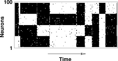
Figure 2: Activity of neurons versus time for $N=100$ neurons and $P=4$ patterns. Here, $T_{0}=0.9T_{0}^{c}$ and $T_{1}=1.69T_{1}^{c}$, where $T_{0}^{c}$ and $T_{1}^{c}$ are the corresponding critical values of temperatures.

One might argue that these jumps are a finite size effect; it does not seem to be the case, however. Similar jumping phenomena, apparently independent of the size of the system,[9] have already been described in kinetic Ising–like models in which disorder is homogeneous in space and varies with time, and mean–field solutions also exhibit these phenomena. Some finite–size effects are evident, however; the synaptic temperature, for instance, scales with size. In fact, we obtain $T_{1}^{c}/N=0.0431\pm 0.0001$ for $N=1024,1600$ and $4096$; consequently, we redefine $\beta_{1}\equiv\beta_{1}N$ from now on.

A series of our computer experiments concerned $N=65536$ and $P=6.$ In order to study in detail the oscillatory phase, it turned out convenient to look at time correlations. Therefore, we used correlated patterns, namely, there was an average overlap of 20% between any two of the stored patterns. The goal was to detect non–trivial correlations between jumps, so that we computed the time $\tau_{\nu\gamma}$ the system remains in pattern $\nu$ before jumping to pattern $\gamma;$ $\sum_{\gamma=1}^{P}\tau_{\nu\gamma}=\tau_{\nu}$ is the total time the system stays in pattern $\nu.$ This reveals the existence of two different kinds of oscillatory behavior. One is such that $\tau_{\nu\gamma}\simeq\tau,$ independent of $\nu$ and $\gamma.$ That is, the system stays the same time at each pattern, so that jumping behaves as a completely random process, without any time correlation. This is denoted by O(II) in Figure $1$ (Left). Even more interesting is phase O(I). As the probability of jumping between patterns is activity dependent, lowering $T_{0}$ leads to non–trivial time correlations, namely, $\tau_{\nu\gamma}$ depends on both $\nu$ and $\gamma.$ We also observe that $\tau_{\nu\gamma}$ differs from $\tau_{\gamma\nu}$. This peculiar behavior suggests one that some spatial temporal information may be coded in phase O(I) .

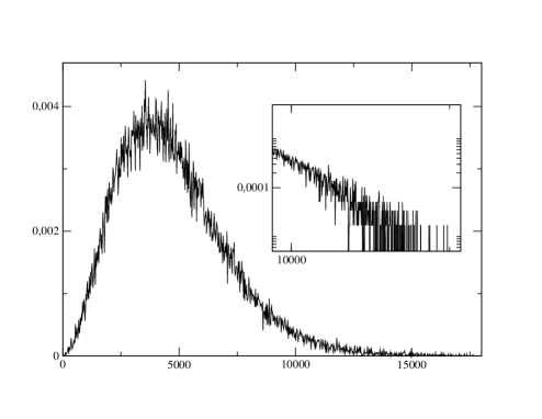
Figure 3: Probability distribution for the time the system stays in a pattern before jumping to another one in the phase O(II). Inset: Tail for large events.

In order to understand further these two different jumping mechanisms, we simulated for $T_{0}=\{0.1,0.5,1.1\}$, in units of $T_{0}^{c},$ at fixed $T_{1}=1.36T_{1}^{c}.$ The resulting probability distribution of time $\tau_{\nu}$ averaged over $\nu,$ $P(\tau),$ is shown in Figure $2$. The data fit $P(\tau)=A\exp(-B\tau^{2})\tau^{2}.$ This predicts that $\langle\tau^{2}\rangle^{2}=\frac{9}{64}\pi^{2}\langle\tau\rangle^{4}$ which compared with our simulations gives relative errors of $e(\%)=\{3.3,3.8,11.2\}$ for $T_{0}=\{0.1,0.5,1.1\}$, respectively. The error increases with $T_{0}$ because the overlaps then tend to become too small and jumps are, consequently, not so well-defined.

Also interesting is the average of time $\tau$ before jumping, because diverging of $\langle\tau\rangle$ indicates that the overlap is stable and no jumps occur. The trial distribution above gives $\langle\tau\rangle=A/2B^{2}.$ Therefore, $B$, which also enters the probability normalization as $A=4(B^{3}/\pi)^{1/2}$, indicates whether there are jumps $(B\neq 0)$ or not $(B=0)$. $B$ measures the jumping frequency.

It is also worth studying the tails of the distributions for large events. This is illustrated in Figure $2$ (Inset) . One may argue that, as in Ref.[10] for somewhat related phenomena, this tail is due to the superposition of many exponentials, each corresponding to a well–defined type of jumping event. We are presently studying this possibility in detail.

We acknowledge P.I. Hurtado for very useful comments and financial support from MCyT-FEDER, project BFM2001-2841 and the J.J.T.’s Ramón y Cajal contract.

References

• [1] L.Β Pantic, J.Β Torres, H.Β Kappen, Associative memory with dynamic synapses, Neural Comp. 14Β (12) (2002) 2903–2923.
• [2] D.Β Horn, M.Β Usher, Neural networks with dynamical thresholds, Phys. Rev. A 40Β (2) (1989) 1036–1044.
• [3] J.Β Marro, R.Β Dickman, Nonequilibrium Phase Transitions in Lattice Models, Cambridge University Press, Cambridge, 1999.
• [4] J.Β Marro, J.Β Torres, P.Β Garrido, Effect of correlated fluctuations of synapses in the performance of neural networks, Phys. Rev. Lett. 81Β (13) (1998) 2827–2830.
• [5] J.Β Torres, P.Β Garrido, J.Β Marro, Neural networks with fast time-variation of synapses, J. Phys. A: Math. and Gen. 30Β (22) (1997) 7801–7816.
• [6] A.Β Coolen, R.Β Penney, D.Β Sherrington, Coupled dynamics of fast and slow interactions: An alternative perspective on replicas, Phys. Rev. B 48Β (21) (1993) 16116–16118.
• [7] A.Β Coolen, HandBook of Biological Physics, Vol.Β 4, Elsevier Science, 2001, Ch. Statistical Mechanics of Recurrent Neural Networks II: Dynamics, pp. 597–662.
• [8] J.M. Cortes etΒ al., To be published.
• [9] J.Β Alonso, M.Β Munoz, Temporally disordered ising models, Europhys. Lett. 56Β (4) (2001) 485–491.
• [10] P.Β Hurtado, J.Β Marro, P.Β Garrido, Origin of avalanches with many scales in a model of disorder. to be published.