A Variational Monte Carlo Study of the Current Carried by a Quasiparticle

Abstract

With the use of Gutzwiller-projected variational states, we study the renormalization of the current carried by the quasiparticles in high-temperature superconductors and of the quasiparticle spectral weight. The renormalization coefficients are computed by the variational Monte Carlo technique, under the assumption that quasiparticle excitations may be described by Gutzwiller-projected BCS quasiparticles. We find that the current renormalization coefficient decreases with decreasing doping and tends to zero at zero doping. The quasiparticle spectral weight $Z_{+}$ for adding an electron shows an interesting structure in $\mathbf{k}$ space, which corresponds to a depression of the occupation number $n_{\mathbf{k}}$ just outside the Fermi surface. The perturbative corrections to those quantities in the Hubbard model are also discussed.

I Introduction

In recent years, it has been acknowledged that ground-state properties of high-temperature superconductors may be reasonably well described with the help of Gutzwiller-projected wave functions Anderson et al. (2004). However the main challenge of any candidate theory of high-temperature superconductivity is the description of finite-temperature properties such as the superconducting transition and the pseudogap phenomenon in underdoped cuprates. One of the first issues related to the finite-temperature physics of high-temperature superconductors is the structure of low-lying excitations. Within the framework of Gutzwiller-projected wave functions, the first steps in studying the excitations have been recently made: the quasiparticle spectrum and the quasiparticle spectral weight have been calculated Paramekanti et al. (2001); Yunoki et al. (2005). In our paper, we complement the previous studies with the analysis of the current carried by the quasiparticles. The magnitude of the quasiparticle current has a direct physical implication in reducing the superfluid density at finite temperature, which eventually determines the superconducting transition temperature in the underdoped regime Lee and Wen (1997); Wen and Lee (1998). Furthermore, the deviation of the quasiparticle current from the prediction of the BCS theory may provide a helpful insight in the physics of high-temperature superconductivity.

The reduction of the superfluid density $n_{s}(T)/m$ by thermal quasiparticles at the nodes of a $d$-wave superconductor has been computed by Lee and Wen Lee and Wen (1997); Wen and Lee (1998) as

$$\frac{\hbar^{2}n_{s}(T)}{m}=\frac{\hbar^{2}n_{s}(0)}{m}-\frac{2\ln 2}{\pi}\alpha^{2}(\frac{v_{F}}{v_{\Delta}})k_{B}T\,,$$ (1)

where $v_{F}$ and $v_{\Delta}$ are the velocity of the nodal quasiparticles perpendicular and parallel to the underlying Fermi surface, and $\alpha$ is the phenomenological Landau parameter Millis et al. (1998) which renormalizes the current carried by the quasiparticle

$$\mathbf{j}(\mathbf{k})=-e\alpha\mathbf{v}_{F}.$$ (2)

Experimentally, $n_{s}(T)/m$ can be related to the London penetration depth $\lambda$, and the ratio $v_{F}/v_{\Delta}$ may be extracted independently from a thermal-conductivity measurement Chiao et al. (2000). This makes $\alpha$ an experimentally accessible quantity for a variety of doping values Liang et al. (2005); Broun et al. .

In the first part of the paper, we focus on computing the current renormalization $\alpha$ for different doping values. We find that it decreases with decreasing doping, and that it is roughly constant along the Fermi surface at all dopings. The contribution of particles and holes to the total quasiparticle current allows us to picture the “effective Fermi surface” where the electron contribution crosses over to the hole contribution. We observe that this “effective Fermi surface” deviates considerably from the original Fermi surface of the unprojected BCS state. This reveals the particle-hole asymmetry produced by the Gutzwiller projection.

In the second part of the paper, we discuss another renormalization parameter: the quasiparticle spectral weight $Z_{+}$ for adding an electron. The momentum dependence of $Z_{+}$ shows a pocket structure at the diagonal of the Brillouin zone just outside the Fermi surface. We further discuss the relations and bounds on $Z_{+}$ in the $t$–$J$ model, as well as corrections arizing from the rotation to the Hubbard model.

For our analysis, we take the minimal two dimensional model for strongly interacting electrons on a lattice, the Hubbard model. Following the usual procedure (see, e.g., Refs. Paramekanti et al., 2001, 2004), we first study the wave function for its strong-coupling limit, the $t$–$J$ model and then include the first-order correction in $t/U$ due to the doubly-occupied sites. The Hamiltonian for the $t$–$J$ model for our system is defined on the two-dimensional square lattice by

$$\mathcal{H}_{tJ} = -t\sum_{\langle i,j\rangle,\sigma}\left(c_{i,\sigma}^{\dagger}c_{j,\sigma}+\mathrm{h.c.}\right)$$ (3)

$$+J\sum_{\langle i,j\rangle}\left(\mathbf{S}_{i}\cdot\mathbf{S}_{j}-n_{i}n_{j}/4\right),$$

with $t/J=3$. Here $c_{i,\sigma}^{\dagger}$ is the electron creation operator at site $i$ with spin $\sigma=(\uparrow,\downarrow)$. The $\langle i,j\rangle$ indicates nearest neighbors, $\mathbf{S}_{i}=\frac{1}{2}c_{i,\alpha}^{\dagger}\vec{\sigma}_{\alpha,\beta}c_{i,\beta}$, and $n_{i}=c_{i,\alpha}^{\dagger}c_{i,\alpha}$. The Hamiltonian (3) is then supplemented with the constraint that no double occupancy is allowed.

We use the variational Monte Carlo technique to calculate expectation values of operators given our trial wave functions. Gros (1989); Yokoyama and Shiba (1988) For the $t$–$J$ model, we consider two related trial wave functions: the ground state wave function $|\Psi_{\mathrm{GS}}\rangle$ and the wave function for the excited state $|\Psi_{\mathrm{EX}}\rangle$. For the ground state, we use the Gutzwiller-projected $d$-wave singlet,

$$|\Psi_{\mathrm{GS}}\rangle=P_{D}P_{N}|\Psi_{\mathrm{BCS}}\rangle$$ (4)

where $P_{D}=\prod_{i}\left[1-n_{i,\uparrow}n_{i,\downarrow}\right]$ is the Gutzwiller projection operator onto the subspace with no doubly occupied states, and $P_{N}$ is the projection operator onto the subspace with $N$ particles. $|\Psi_{\mathrm{BCS}}\rangle=\prod_{\mathbf{k}}\left[1+a_{\mathbf{k}}c_{\mathbf{k},\uparrow}^{\dagger}c_{-\mathbf{k},\downarrow}^{\dagger}\right]|0\rangle$, where $c_{\mathbf{k},\sigma}^{\dagger}$ is the Fourier transform of real-space electron creation operator $c_{i,\sigma}^{\dagger}$. Following the standard BCS definitions for a $d$-wave singlet state,

$$a_{\mathbf{k}} =\frac{v_{\mathbf{k}}}{u_{\mathbf{k}}}=\frac{\Delta_{\mathbf{k}}}{\xi_{\mathbf{k}}+\sqrt{\xi_{\mathbf{k}}^{2}+\Delta_{\mathbf{k}}^{2}}},$$ (5)

$$\Delta_{\mathbf{k}} =\Delta_{\mathrm{var}}(\cos{k_{x}}-\cos{k_{y}}),$$ (6)

$$\xi_{\mathbf{k}} =\varepsilon_{\mathbf{k}}-\mu_{\mathrm{var}},$$ (7)

with $\varepsilon_{\mathbf{k}}=-2(\cos{k_{x}}+\cos{k_{y}})$. Not only has this $d$-wave Gutzwiller-projected wave function been shown to give good variational energies for the $t$–$J$ model relative to other possible phases, but also it has correctly reproduced many properties of the superconducting state.Yokoyama and Ogata (1996); Paramekanti et al. (2001)

For the trial wavefunction of the low-lying excited states, we take the natural ansatz of the Gutzwiller-projected Bogoliubov quasiparticle (Anderson (1987); Yunoki et al. (2005))

$$|\Psi_{\mathrm{EX}}(\mathbf{k},\sigma)\rangle=P_{D}P_{N}\gamma_{\mathbf{k},\sigma}^{\dagger}|\Psi_{\mathrm{BCS}}\rangle.$$ (8)

Since the overall normalization of the wave function is of no importance, we may also rewrite the trial excited state as

$$|\Psi_{\mathrm{EX}}(\mathbf{k},\sigma)\rangle=P_{D}P_{N}c_{\mathbf{k},\sigma}^{\dagger}|\Psi_{\mathrm{BCS}}\rangle.$$ (9)

Throughout the paper, we suppress the $\mathbf{k}$ and $\sigma$ variables on $|\Psi_{\mathrm{EX}}\rangle$ for notational convenience. The expectation values of any operator $\mathcal{O}$ in the variational ground and excited states will be often denoted as $\langle\mathcal{O}\rangle_{\mathrm{GS}}$ and $\langle\mathcal{O}\rangle_{\mathrm{EX}}$ respectively.

In our simulations, we use the optimal values of $\Delta_{\mathrm{var}}$ and $\mu_{\mathrm{var}}$ calculated for the ground state trial wave function Ivanov and Lee (2003), both for the ground state and for the excited state. These values minimize the expectation value $\langle\mathcal{H}_{tJ}\rangle_{\mathrm{GS}}$ of the physical $t$–$J$ Hamiltonian at a fixed concentration of holes.

We assume boundary conditions that are anti-periodic in the $x$ direction and periodic in the $y$ direction so that we avoid the singularity in $a_{\mathbf{k}}$ along the nodal diagonal, $(0,0)$ to $(\pi,\pi)$. A drawback of this choice of boundary conditions is that we are unable to calculate quantities exactly on the nodal diagonal, and instead calculate expectation values for nearby $\mathbf{k}$ points. This becomes an important source of error when we compute expectation values at the nodal point. We try to lower this error by looking at larger systems in order to get better resolution; however, we are limited by our computing resources.

This trial excited state and various related ones have been studied previously by other groups Giamarchi and Lhuillier (1993); Lee and Shih (1997); Lee et al. (2003); Yunoki et al. (2005). The energy dispersion of the low-energy quasiparticles has been found to be of the BCS type $E(\mathbf{k})=\left[\xi^{2}+\Delta_{\mathbf{k}}^{2}\right]^{1/2}$, but with renormalized values of the gap and bandwidth. The nodal point obviously coincides with the nodal point of the unprojected wave function $\Psi_{\mathrm{BCS}}$ and slowly shifts inwards from $(\pi/2,\pi/2)$ along the diagonal of the Brillouin zone as the hole doping increases.

II CURRENT CARRIED BY THE QUASIPARTICLES

In this section, we investigate the current carried by quasiparticles as a function of their momenta and doping. The current carried by the excited state $|\Psi_{\mathrm{EX}}(\mathbf{k},\sigma)\rangle$ is defined as

$$\langle\mathbf{j}_{\mathbf{k},\sigma}\rangle=\langle\sum_{\langle ij\rangle,\alpha}it(c_{\alpha,i}^{\dagger}c_{\alpha,j}-c_{\alpha,j}^{\dagger}c_{\alpha,i})\rangle_{\mathrm{EX}},$$ (10)

where $\langle ij\rangle$ represents a sum over all links. Note that the orientation and direction of the link determines its contribution to the vector $\mathbf{j}$. We can interpret the excited state trial wave function as the ground state for a system of $N$ particles to which we add one unpaired electron so that our state has a net spin and charge. The Gutzwiller projection enforces strong correlation between the added electron and the $N$-electron ground state, so that we expect an effective quasiparticle with renormalized parameters.

Figure 1: The top middle and bottom figures are respectively plots of the current $\mathbf{j}$, $\mathbf{j_{\uparrow}}$, and $\mathbf{j_{\downarrow}}$ as a function of the wavevector $\mathbf{k}$ for a 12$\times$12 system with 13 holes, $x=0.09$. The vectors are drawn starting at the $\mathbf{k}$-point at which the current is calculated, their length is proportional to the current magnitude.

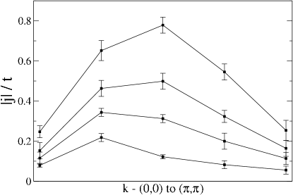
Figure 2: The magnitude of the current $\left|\mathbf{j}\right|$ measured in units of $t$ along the nodal diagonal, $(0,0)$ to $(\pi,\pi)$. These runs were done on the 10$\times$10 system with the doping of 0.01, 0.05, 0.09 and 0.17 (increasing magnitude).

In the standard BCS theory (without the Gutzwiller projection), the current carried by the quasiparticles is $\mathbf{j}_{\mathbf{k}}=e\mathbf{v}_{\mathbf{k}}$ where $\mathbf{v}_{\mathbf{k}}=d\varepsilon_{\mathbf{k}}/d\mathbf{k}$ is the velocity from the underlying normal state and not the velocity from the quasiparticle dispersion $dE/d\mathbf{k}$. This is the result of the fact that in BCS theory the excitations are a superposition of particle and hole states and that these states carry opposite charge but also move in opposite directions. The underlying metallic state can have some Fermi liquid correction to the current carried by the particles and holes. This correction is then carried through to the quasiparticle current in the superconducting state, $\mathbf{j}_{\mathbf{k}}=\alpha e\mathbf{v}_{\mathbf{k}}$. In the case of the Gutzwiller projected trial excited state that we are studying, we see that current does still approximately follow the shape of the dispersion of the underlying metal and that the quasiparticle current renormalization $\alpha$ can be calculated from the ratio of $\mathbf{j}/\mathbf{v}_{\mathbf{k}}$.

II.1 Current as a function of k

First we examine $\mathbf{j}$, the current carried by the quasiparticle, as a function of $\mathbf{k}$ for various dopings. At most dopings, we find a distribution with a structure similar to what one would expect from the tight binding model. In the top plot of Fig. 1, a typical example of the current carried by the quasiparticle as a function of wavevector is plotted. We compare the direction of the current as a function of momentum to both the quasiparticle dispersion, $dE(\mathbf{k})/d\mathbf{k}$, and to the underlying dispersion of the normal state $\mathbf{v}_{\mathbf{k}}$. We find that the shape of the current indeed approximately follows the dispersion of the normal state and not the dispersion of the quasiparticles. This is the same as in the BCS theory so the Gutzwiller projection does not change this aspect of the physics.

For intermediate doping values, the magnitude of the current reaches its maximum value near the center of the Brillouin zone, and therefore near the nodal point. However, for strongly underdoped simulations, $x<0.05$, we find that the maximum moves inward along the nodal direction, becoming closer to $(\pi/4,\pi/4)$ as the doping approaches zero. (See Fig. 2)

We also look at how much of the total current is being carried by the up spins and down spins individually. By restricting the $\sum_{\alpha}$ in equation 10 so that we consider $\alpha=\uparrow$ and $\alpha=\downarrow$ separately, we can investigate this property of our trial excited state. Since we are now distinguishing between these two spins, it is important to note that we define our trial wave function as adding an up-spin to the system. Given this, we find that the current of our state is almost entirely carried by either the up spins or the down spins depending on whether or not we are inside or outside of the effective Fermi surface as can be seen in the lower two plots of Fig. 1. Inside of the Fermi surface, all of the current is carried by the down spins and outside of the Fermi surface all of the current is carried by the up spins. This is the qualitatively the same as in the unprojected case where the up and down spin currents have factors of $u_{\mathbf{k}}^{2}$ and $v_{\mathbf{k}}^{2}$ respectively.

Figure 3: The particle contribution to the quasiparticle current $n_{\mathbf{j}}(\mathbf{k})$ defined in Eq. (11). The top and the bottom plots correspond to 13 and 31 holes in the 12$\times$12 system (doping $x=0.09$ and $x=0.22$, respectively). The contour lines are $n_{\mathbf{j}}(\mathbf{k})=0.1$, 0.3, 0.5, 0.7, and 0.9 (from left to right). The thick dashed line is the Fermi surface of the unprojected state, the thick solid dot marks the position of the node. Small crosses indicate the positions of data points (we have used the reflection about the $x$–$y$ diagonal to double the density of data points).

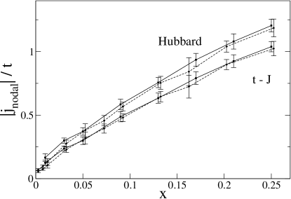
Figure 4: Magnitude of the nodal current, $\left|\mathbf{j}_{\mathrm{nodal}}\right|$ measured in units of $t$, plotted as a function of doping. The solid lines are the data from a 10$\times$10 lattice and the dashed lines from a 20$\times$20 one. The lower curves are for the trial wavefunction for the $t$–$J$ model and the upper curves are for the trial wavefunction for the Hubbard model (to the lowest order in $t/U=1/12$).

To make a more detailed comparison to the BCS theory, we define the “particle contribution” to the current as

$$n_{\mathbf{j}}=\frac{\mathbf{j}_{\downarrow}(\mathbf{k})\cdot\mathbf{j}_{\mathrm{t}ot}(\mathbf{k})}{|\mathbf{j}_{\mathrm{t}ot}(\mathbf{k})|^{2}}\,,$$ (11)

where $\mathbf{j}_{\mathrm{t}ot}=\mathbf{j}_{\downarrow}+\mathbf{j}_{\uparrow}$ is the total current carried by the quasiparticle. In the BCS theory, $n_{\mathbf{j}}(\mathbf{k})=|v_{\mathbf{k}}|^{2}$, it takes the values between zero and one, and the isoline $n_{\mathbf{j}}(\mathbf{k})=0.5$ coincides with the Fermi surface. In Fig. 3 we show the contour plots of $n_{\mathbf{j}}(\mathbf{k})$ for different values of doping, together with the Fermi surface for the corresponding unprojected BCS wave functions. We see that the “effective Fermi surface” defined by $n_{\mathbf{j}}(\mathbf{k})$ does not follow the original Fermi surface of the BCS state, but bends outwards in the $(0,\pi)$ regions. Thus it effectively acquires an inward curvature similar to the effect of the negative $t^{\prime}$ hopping term.

II.2 Current as a function of doping

We noted earlier that the magnitude of the current has a maximum near the nodal point and that this maximum decreases as a function of doping. In Fig. 4, we plot the magnitude of the nodal current $\mathbf{j}_{\mathrm{nodal}}=\mathbf{j}(\mathbf{k}=(\pi/2,\pi/2))$ versus doping for both 10$\times$10 and 20$\times$20 systems. Because of our choice of boundary conditions, we do not calculate the current at the true nodal point. For a 10$\times$10 system, the “nodal point” is actually evaluated at $\mathbf{k}=(0.5\pi,0.4\pi)$ and for a 20$\times$20 system at $\mathbf{k}=(0.45\pi,0.5\pi)$. In Fig. 4, we see that there is agreement to within the error between the data calculated for two lattices of different size, and we expect that the actual nodal current would also be within these errors.

In the 20$\times$20 system, we can study the doping as low as 0.005 (2 holes), and our results indicate that the current apparently decreases down to zero with decreasing doping.

II.3 Rotation to the Hubbard model

So far we have studied the properties of fully projected wave functions. We would now like to extend our simulations from the $t$–$J$ model back to the Hubbard model. This can be done in the standard way by employing a unitary transformation $e^{iS}$ that decouples the Hilbert space of the Hubbard Hamiltonian so that there are no matrix elements connecting those subspaces with different numbers of doubly occupied sites. Following MacDonald et al.MacDonald et al. (1988), we determine this transformation as a power series in $(t/U)$, so that the subspaces are decoupled order by order. To the first order, the rotation generator is given by

$$iS=\frac{1}{U}\left(T_{1}-T_{-1}\right)\,,$$ (12)

where $T_{1}$ and $T_{-1}$ are defined to be the parts of the kinetic energy operator that increase and decrease, respectively, the number of doubly occupied sites by one.

With the use of this rotation, we can replace computing the expectation value of any operator $O$ in the ground state of a Hubbard model by computing the expectation value of the rotated operator $\langle e^{iS}Oe^{-iS}\rangle$ in the ground state of the $t$–$J$ model. We use the same variational wave function for the $t$–$J$ model as described above and compute the lowest-order correction (linear in $t/U$) to the $t$–$J$ expectation value. This procedure has been applied, for example, in the work of Paramekanti et al. Paramekanti et al. (2004) for calculating the expectation value of the occupation-number operator.

We compute the rotation correction to the value of the nodal current and find that it does not qualitatively change its doping dependence. The corrected value of the current is plotted as the upper curves in Fig. 4 (for $t/U=1/12$)

II.4 Quasiparticle current renormalization $\alpha$

Beyond just studying the current itself, we are particularly interested in the quasiparticle current renormalization factor $\alpha$. As we noted earlier the current and the slope of the dispersion are collinear within the error of our simulations, so we can define $\alpha=\mathbf{j}/\mathbf{v}_{\mathbf{k}}$.

We look at the quasiparticle current renormalization parameter $\alpha$ as a function of doping. We are interested in $\alpha$ for the lowest lying excitations, i.e., for those at the nodal point. Although we have calculated the Fermi velocity at the nodal point, more precise data for this velocity as a function of doping are available from the work by Yunoki et al. Ref. Yunoki et al. (2005). We use those Fermi velocity data in conjunction with our nodal current results to calculate $\alpha$ at the nodal point.

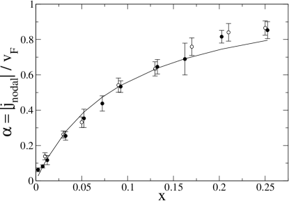
Figure 5: The renormalization of the quasiparticle current $\alpha=|\mathbf{j}_{\mathrm{nodal}}|/v_{F}$ as a function of doping. The open circles are for runs on a 10$\times$10 lattice and the solid ones are for runs on a 20$\times$20 one. The solid line is the fit to the 20$\times$20 data by Eq. (16) at $x^{*}=0.09$.

In Fig. 5, we plot the nodal value of $\alpha$ as a function of doping. We find that $\alpha$ goes to zero at zero doping.

It is interesting to compare our results with the predictions of slave-boson theory. In this theory, the low lying excitations are $x$ bosons which carry charge with an effective hopping matrix element proportional to $t$ and fermions which carry spin with an effecting hopping proportional to $J$. These excitations are coupled to gauge fluctuations. When the gauge fluctuations are treated at the Gaussian level, we obtain the Ioffe–Larkin composition rule which states that the inverse of the superfluid density $\rho_{s}=n_{s}/m$ is given by adding the inverses of the fermion and boson contributions:

$$\rho_{s}^{-1}=(\rho_{s}^{F})^{-1}+(\rho_{s}^{B})^{-1}$$ (13)

where $\rho_{s}^{B}\approx xt$ and $\rho_{s}^{F}\approx J(1-aT)$ with $a\approx\Delta^{-1}$. Ioffe and Larkin (1989) Note that the linear temperature dependence comes from thermal excitations of the nodal fermions. Expanding Eq. 13 at small $T$, we obtain

$$\rho_{s}(T)\approx\rho_{s}(0)-\frac{[\rho_{s}(0)]^{2}}{\rho_{s}^{F}(0)}aT\,.$$ (14)

On the other hand, the quasiparticle dispersion is given by that of the fermions and we can identify $v_{F}/v_{\Delta}$ in Eq. 1 as being proportional to $aJ\sim a\rho_{s}^{F}(0)$. Comparison of Eq. 14 with Eq. 1 results in the simple expression

$$\alpha\sim\frac{\rho_{s}(0)}{\rho_{s}^{F}(0)}\,,$$ (15)

in particular $\alpha\propto x(t/J)$ for $xt<J$. Lee et al. (To Be Published) We did not keep track of the numerical coefficients. If we assume that at full doping ($x=1$) $\alpha$ should approach one (the BCS value), Eq. (15) suggests the form

$$\alpha(x)=\frac{x}{x+x^{*}}(1+x^{*})\,,$$ (16)

which for $x^{*}=0.09$ produces a qualitatively good fit of our results for $\alpha$ (see Fig. 5). Note that the order-of-magnitude estimates above gives $x^{*}\sim J/t$, and our best-fit value of $x^{*}$ is several times smaller.

The shape and the magnitude of the current renormalization parameter $\alpha$ as a function of doping is currently a topic of much experimental work. While there still remain large uncertainties in the experimental data, two useful comparisons can be made to our work. In Ref. Chiao et al., 2000, the measurements of thermal conductivity and of the penetration depth were used to determine the ratio $v_{F}/v_{\Delta}$ and the superfluid density. Combining those data resulted in the the values of $\alpha=0.66$ and $\alpha=0.68$ for optimally doped samples of BSCCO and YBCO, respectively. Those numbers are in close agreement with our results around $x=0.15$ doping.

Our results also qualitatively agree with the decrease of $\alpha$ as the doping decreases in underdoped YBCO, as reported in Refs. Liang et al., 2005; Broun et al., . However, earlier data on YBCO films indicated that the linear $T$ slope of $n_{s}/m$ is relatively insensitive to doping over a broad range of critical temperatures. Boyce et al. (2000); Stajic et al. (2003) Since $v_{F}/v_{\Delta}$ decreases with decreasing $x$ Sutherland et al. (2003), this trend is in disagreement with Fig. 5 and Eq. (16). It will be desirable to have single crystal data for $n_{s}(T)/m$ over a broad range of $x$ to settle this point.

On the theoretical side, the recent study of a $U(1)$ slave-boson theory with spinon-holon binding Ng (2005) predicted a sub-linear dependence of $\alpha$ on the doping. The sublinear form of $\alpha(x)$ disagrees with our proposal (16), but is also consistent with our numerical results shown in Fig. 5.

We further look at $\alpha$ along the Fermi surface for a given doping. We are interested in how the shape and size of this curve changes as a function of doping. While we expect the integral of the whole curve to decrease with $x$, there are several possibilities for how this could occur. Two such scenarios are that the curve decreases in magnitude everywhere along the Fermi surface uniformly as doping decreases or that $\alpha$ is small almost everywhere along the Fermi surface but that there is a region of large $\alpha$ around the nodal point whose width increases with $x$. Our numerical results indicate the former of those scenarios. In the upper graph of Fig. 6, we plot the $t$–$J$ model current magnitude along the Fermi surface. Due to the low finite resolution of our system, we just calculate the current at those points nearest to the line connecting $(\pi,0)$ and $(0,\pi)$. To calculate $\alpha$, we use the value of $v_{F}$ found by Yunoki et al. Yunoki et al. (2005) along the nodal direction for a given doping and accordingly renormalize the tight binding dispersion to calculate $\mathbf{v}_{\mathbf{k}}$ along these points. We plot $\alpha$ obtained in this way in the lower plot of Fig. 6. We see that $\alpha$ is approximately flat along the Fermi surface.

$\_$

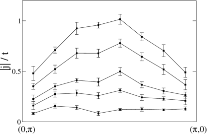
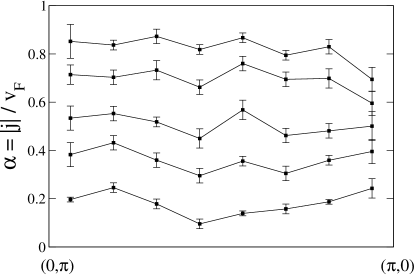
Figure 6: Plot of $\left|\mathbf{j}\right|$ and $\alpha=\left|\mathbf{j}\right|/v_{F}$, upper and lower plots respectively, for the $t$–$J$ model along the Fermi surface for dopings of 0.01,0.05,0.09,0.17 and 0.25 (increasing magnitude).

III Quasiparticle weight and Occupation Number

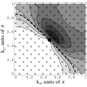
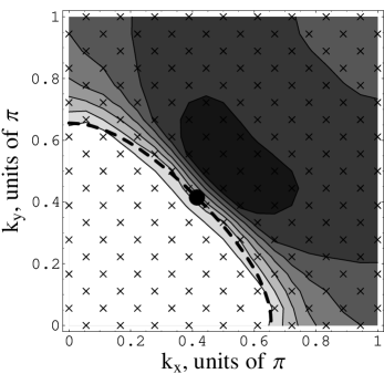
Figure 7: Contour plots of $Z_{+}(\mathbf{k})$ in the $t$–$J$ model for dopings 0.03 (upper plot) and 0.21 (lower plot), 10 and 68 holes in a 18$\times$18 system, respectively. The thick dashed lines denote the Fermi surface of the unprojected wave function, the big solid dot marks the position of the node. Crosses indicate data points used in plotting (available values of the $\mathbf{k}$ vector). In the upper plot, the contour lines correspond to $Z_{+}=0.01$, $0.02$, $\dots$, $0.09$ (left to right – the maximal value of $Z_{+}$ is $0.09$). In the lower plot, the contour lines are $Z_{+}=0.05$, $0.10$, $\dots$, $0.35$ (with the maximal value $Z_{+}=0.38$).

In this section we examine the quasiparticle weight $Z$ and the occupation number $n$ as a function of momentum and doping. The quasiparticle weight is defined as in Fermi liquid theory and gives a measure of how close our trial wave function quasiparticle is to being a free electron (or a free hole).

We begin with the definitions,

$$Z_{+}(\mathbf{k},\sigma)=\frac{\left|\langle\Psi_{\mathrm{EX}}|c_{\mathbf{k},\sigma}^{\dagger}|\Psi_{\mathrm{GS}}\rangle\right|^{2}}{\langle\Psi_{\mathrm{EX}}|\Psi_{\mathrm{EX}}\rangle\langle\Psi_{\mathrm{GS}}|\Psi_{\mathrm{GS}}\rangle}\,,$$ (17)

$$Z_{-}(\mathbf{k},\sigma)=\frac{\left|\langle\Psi_{\mathrm{EX}}|c_{\mathbf{k},\sigma}|\Psi_{\mathrm{GS}}\rangle\right|^{2}}{\langle\Psi_{\mathrm{EX}}|\Psi_{\mathrm{EX}}\rangle\langle\Psi_{\mathrm{GS}}|\Psi_{\mathrm{GS}}\rangle}\,,$$ (18)

where $|\Psi_{\mathrm{EX}}\rangle$ also carries momentum $\mathbf{k}$, and the electron operators are normalized as $\{c_{\mathbf{k},\sigma},c_{\mathbf{k},\sigma}^{\dagger}\}=1$. In the BCS theory (without Gutzwiller projection), $Z_{+}=u_{\mathbf{k}}^{2}$ and $Z_{-}=v_{\mathbf{k}}^{2}$. Along the nodal diagonal (where the gap vanishes), $u_{\mathbf{k}}^{2}=1$ outside the Fermi surface and $0$ inside and $v_{\mathbf{k}}^{2}$ is the opposite. If one defines $Z=Z_{+}+Z_{-}$, then in the BCS model $Z=1$ everywhere.

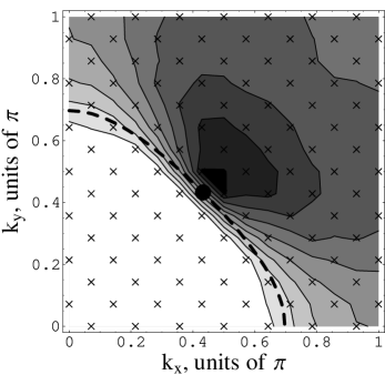
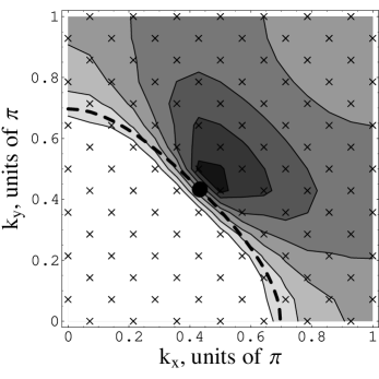
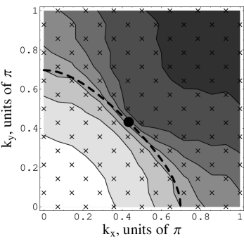
Figure 8: Upper plot: contour plot of $Z_{+}(\mathbf{k})$ (or, equivalently, of $n(\mathbf{k})$) in the $t$–$J$ model at the doping 0.12 (24 holes in the 14$\times$14 system). The isolines correspond to $Z_{+}=0.03,0.06,\dots,0.27$ [$n(\mathbf{k})=0.53,0.50,\dots,0.29$ respectively, left to right]. The maximal value of $Z_{+}$ (near the node) is $0.27$. Middle plot: $Z_{+}^{H}$ in the same system rotated to the Hubbard model (to the first order in $t/U=1/12$), Eq. (28). The isolines correspond to $Z_{+}^{H}=0.05,0.10,\dots,0.35$. The maximal value of $Z_{+}^{H}$ (near the node) is $0.37$. Bottom plot: $n_{\mathbf{k}}^{H}$ in the same system rotated to the Hubbard model (to the first order in $t/U=1/12$), Eq. (29). The isolines are $n_{\mathbf{k}}^{H}=0.8,0.7,\dots,0.2$ (left to right). The Fermi surface, the nodal point and the positions of data points are denoted in the same way as in Fig. 7.

In the projected wave functions, these simple expressions do not apply. However, some of the properties of the spectral weights $Z_{+}$ and $Z_{-}$ may be still proven. Using the identity

$$P_{D}c_{k}^{\dagger}P_{D}=P_{D}c_{k}^{\dagger}$$ (19)

and the $d$-wave symmetry of the gap, we can prove that along the nodal diagonal,

$$Z_{+}=0 {}\quad{\rm on}\quad{} (0,0)-(k_{F},k_{F})\,,$$ (20)

$$Z_{-}=0 {}\quad{\rm on}\quad{} (k_{F},k_{F})-(\pi,\pi)\,,$$ (21)

where $(k_{F},k_{F})$ is the nodal point. Furthermore, $Z_{+}$ may be rewritten as the ground-state expectation value

$$Z_{+}(\mathbf{k},\sigma)=\langle c_{\mathbf{k},\sigma}P_{D}c_{\mathbf{k},\sigma}^{\dagger}\rangle_{\mathrm{GS}}.$$ (22)

We note that

$$\langle c_{i,\sigma}c_{j,\sigma}^{\dagger}\rangle_{\mathrm{GS}} = \langle c_{i,\sigma}Pc_{j,\sigma}^{\dagger}\rangle_{\mathrm{GS}}\quad i\not=j$$ (23)

$$= \langle c_{i,\sigma}Pc_{j,\sigma}^{\dagger}\rangle_{\mathrm{GS}}+n_{\overline{\sigma}}\quad i=j.$$ (24)

Thus $Z_{+}({\mathbf{k},\sigma})$ is further related to the occupation number

$$n_{\mathbf{k},\sigma}=\langle c_{\mathbf{k},\sigma}^{\dagger}c_{\mathbf{k},\sigma}\rangle$$ (25)

as

$$Z_{+}(\mathbf{k},\sigma)=\frac{1+x}{2}-n_{\mathbf{k},\sigma}\,.$$ (26)

This relation has also been given by Yunoki in Ref. Yunoki, . In particular, from this relation follows the upper bound on the spectral weight $Z_{+}$:

$$Z_{+}\leq\frac{1+x}{2}$$ (27)

and, as a consequence, the same upper bound applies to the nodal spectral weight $Z_{\rm nodal}=Z_{+}(k_{F}+\epsilon,k_{F}+\epsilon)$ studied by Paramekanti et al. in Refs. Paramekanti et al., 2001, 2004.

The quasiparticle weight $Z_{-}$ requires a more complicated Monte Carlo calculation, since it cannot be rewritten as a simple ground-state average like (22). We therefore restrict ourselves to discussing only the quasiparticle weight $Z_{+}$ in this paper.

The above relations for $Z_{+}$ have been derived for the fully projected wave function. If we perform a rotation to the Hubbard model, the relations (22) and (26) no longer hold, and the upper bound (27) cannot be proven. Specifically, for the Hubbard model we keep the same definitions of the quasiparticle weights and the occupation number (17), (18), (25), but with the ground and excited states rotated from the fully-projected state to the Hubbard-model state by the unitary rotation $e^{-iS}$, as explained in the previous section. Then the lowest-order Hubbard-model corrections to $Z_{+}$ and to $n_{\mathbf{k}}$ may be easily computed as

$$Z_{+}^{H}=Z_{+}+2\;{\rm Re}\;\langle c_{\mathbf{k},\sigma}P_{D}[iS,c^{\dagger}_{\mathbf{k},\sigma}]\rangle$$ (28)

and

$$n_{\mathbf{k}}^{H}=n_{\mathbf{k}}-2\;{\rm Re}\;\langle c_{\mathbf{k},\sigma}[iS,c^{\dagger}_{\mathbf{k},\sigma}]\rangle\,.$$ (29)

Even though the two expressions look nearly identical, the correction to $n_{\mathbf{k}}$ does not contain an intermediate projector $P_{D}$ and, because of that, has a very different structure than that to $Z_{+}$. The relation between $Z_{+}$ and $n_{\mathbf{k}}$ (26) no longer holds for the Hubbard model, as we shall see below.

Figs. 7 and 8 show $Z_{+}(\mathbf{k})$ for $x=0.03$, $0.12$, and $0.21$. As noted in Eq. (20), $Z_{+}$ is zero along the diagonal between $(0,0)$ and $(k_{F},k_{F})$ and jumps to a finite value $Z_{\mathrm{nodal}}$ at the nodal point. The projected wave function inherits the essential singularity of $Z_{+}$ at the nodal point from the underlying BCS wave function. The value of $Z_{\mathrm{nodal}}$ has been studied as a function of doping by Paramekanti et al. in Refs. Paramekanti et al., 2001, 2004. The doping dependence of $Z_{\mathrm{nodal}}$ (Fig. 2 of Ref. Paramekanti et al., 2001 and Fig. 6 of Ref. Paramekanti et al., 2004) is qualitatively similar to that we find for $\alpha$ (Fig. 5): both $Z_{\mathrm{nodal}}$ and $\alpha$ decrease to zero with decreasing doping, with a strong upward curvature. However we are not aware of any a priori relation between $\alpha$ and $Z_{\mathrm{nodal}}$.

Using (26), the plots of $Z_{+}(\mathbf{k})$ may also be interpreted as those of $n_{\mathbf{k}}$ (see, e.g., the upper plot in Fig. 8). Note the region of depression in $n_{\mathbf{k}}$ just outside the Fermi surface, which resembles a hole “pocket.” The existence of this pocket may already be inferred from the non-monotonous behavior of $n_{\mathbf{k}}$ along the zone diagonal found in Refs. Paramekanti et al., 2001, 2004 but the full $\mathbf{k}$ dependence shown in Figs. 7 and 8 gives a more complete picture. Remarkably, a similar “pocket” structure has been found in the $U(1)$ slave-boson model with spinon-holon-binding by Ng Ng (2005). The pocket is more pronounced at lower dopings and appears consistent with the bending of the “effective Fermi surface” defined in Section II from $n_{\mathbf{j}}$, Eq. 11. However, to define a meaningful Fermi surface from the quasiparticle spectral weight, one needs an access also to the spectral weight $Z_{-}$ which goes beyond the scope of the present paper.

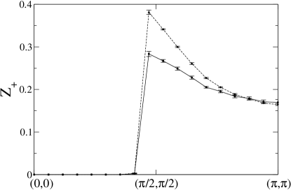
Figure 9: Plot of $Z_{+}$ and $Z_{+}^{H}$, the solid and dashed lines respectively, for an 18$\times$18 system with 40 holes, $x=0.12$. The data are calculated on the discrete grid points closest to the diagonal.

If we include the $t/U$ correction from the rotation to the Hubbard model, the pocket structure in $n_{\mathbf{k}}^{H}$ disappears, see our Fig. 8 (lower plot) and Refs. Paramekanti et al., 2001, 2004. On the other hand, including the $t/U$ correction to $Z_{+}({\mathbf{k}})$ preserves the pocket structure, see Fig. 8 (middle plot). This shows that in the Hubbard model the relation (26) between $Z_{+}^{H}({\mathbf{k}})$ and $n_{\mathbf{k}}^{H}$ no longer holds.

In Refs. Paramekanti et al., 2001, 2004, it was reported that the rotation to the Hubbard model does not change the magnitude of the the jump in $n_{\mathbf{k}}$ at the Fermi surface. Our results on $n_{\mathbf{k}}$ and $n_{\mathbf{k}}^{H}$ confirm this statement, however the spectral weight defined as $Z_{+}$ increases when rotated to the Hubbard model. In Fig. 9, we show $Z_{+}$ and $Z_{+}^{H}$ along the nodal diagonal for an $x=0.12$ system.

IV Conclusion

In this paper, we have analyzed the properties of the excited states in the $t$–$J$ and Hubbard models in the framework of Gutzwiller-projected variational wave functions. The quantities of main interest are the renormalization of the current and spectral weight of the quasiparticles. Both those renormalizations decrease with decreasing doping and exhibit strongly non-BCS behavior.

The renormalization of the quasiparticle current allows us to define the effective Fermi surface as a crossover region between the electron- and hole-supported current. We observe that such a Fermi surface bends outwards in the $(0,\pi)$ regions – an effect normally ascribed to the $t^{\prime}$ hopping term. At the same time, the total current is renormalized approximately uniformly along the Fermi surface.

The renormalization of the quasiparticle spectral weight, on the other hand, is peaked near the nodal point and exhibits a pocket-like structure. This pocket feature is more pronounced at lower doping values.

Comparing the results for the $t$–$J$ model and for the Hubbard model (to the lowest order in the $t/U$ correction), we find that the rotation to the Hubbard model does not qualitatively affect the renormalizations of the quasiparticle spectral weight and of the current.

We would like to thank Professor T.K. Lee and Professor Castellani for their discussions and help on this research. C.P.N. and P.A.L. acknowledge support by NSF grant DMR-0517222.

References

- Anderson et al. (2004) P. W. Anderson, P. A. Lee, M. Randeria, T. M. Rice, N. Trivedi, and F. C. Zhang, J. Phys. Condens. Matter 16, R755 (2004).
- Paramekanti et al. (2001) A. Paramekanti, M. Randeria, and N. Trivedi, Phys. Rev. Letters 87, 217002 (2001).
- Yunoki et al. (2005) S. Yunoki, E. Dagotto, and S. Sorella, Phys. Rev. Lett. 94, 037001 (2005).
- Lee and Wen (1997) P. A. Lee and X. G. Wen, Phys. Rev. Letters 78, 4111 (1997).
- Wen and Lee (1998) X. G. Wen and P. A. Lee, Phys. Rev. Letters 80, 2193 (1998).
- Millis et al. (1998) A. J. Millis, S. M. Girvin, L. B. Ioffe, and A. I. Larkin, J. Phys. Chem. Solids 59, 1742 (1998).
- Chiao et al. (2000) Chiao, Hill, Lupien, Taillefer, Lambert, Gagnon, and Fournier, Phys. Rev. B 62, 3554 (2000).
- Liang et al. (2005) R. Liang, D. A. Bon, W. N. Hardy, and D. Broun, Phys. Rev. Letters 94, 117001 (2005).
- (9) D. Broun, P. Turner, W. A. Huttema, S. Özcan, B. Morgan, R. Liang, W. N. Hardy, and D. A. Bonn, cond-mat/0509223.
- Paramekanti et al. (2004) A. Paramekanti, M. Randeria, and N. Trivedi, Phys. Rev. B 70, 054504 (2004).
- Gros (1989) C. Gros, Ann. Phys 189, 53 (1989).
- Yokoyama and Shiba (1988) H. Yokoyama and H. Shiba, J. Phys. Soc. Jpn. 57, 2482 (1988).
- Yokoyama and Ogata (1996) H. Yokoyama and M. Ogata, J. Phys. Soc. Jpn 65, 3615 (1996).
- Anderson (1987) P. W. Anderson, Science 235, 1196 (1987).
- Ivanov and Lee (2003) D. A. Ivanov and P. A. Lee, Phys. Rev. B 68, 132501 (2003).
- Giamarchi and Lhuillier (1993) T. Giamarchi and C. Lhuillier, Phys. Rev. B 47, 2775 (1993).
- Lee and Shih (1997) T. K. Lee and C. T. Shih, Phys. Rev. B 55, 5983 (1997).
- Lee et al. (2003) W. Lee, T. K. Lee, C. Ho, and P. W. Leung, Phys. Rev. Letters 91, 057001 (2003).
- MacDonald et al. (1988) A. H. MacDonald, S. M. Girvin, and D. Yoshioka, Phys. Rev. B 37, 9753 (1988).
- Ioffe and Larkin (1989) L. Ioffe and A. Larkin, Phys. Rev. B 39, 8988 (1989).
- Lee et al. (To Be Published) P. A. Lee, N. Nagaosa, and X. G. Wen, Rev. Mod. Phys. (To Be Published).
- Boyce et al. (2000) B. R. Boyce, J. Skinta, and T. Lemberger, Physica C 341-348, 561 (2000).
- Stajic et al. (2003) J. Stajic, A. Iyengar, K. Levin, B. Boyce, and T. Lemberger, Phys. Rev. B 68, 024520 (2003).
- Sutherland et al. (2003) M. Sutherland, D. G. Hawthorn, R. W. Hill, F. Ronning, S. Wakimoto, H. Zhang, C. Proust, E. Boaknin, C. lupien, L. Taillefer, et al., Phys. Rev. B 67, 174520 (2003).
- Ng (2005) T.-K. Ng, Phys. Rev. B 71, 172509 (2005).
- (26) S. Yunoki, cond-mat/0508015.