Multifractal PDF analysis for intermittent systems

Abstract

The formula for probability density functions (PDFs) has been extended to include PDF for energy dissipation rates in addition to other PDFs such as for velocity fluctuations, velocity derivatives, fluid particle accelerations, energy transfer rates, etc, and it is shown that the formula actually explains various PDFs extracted from direct numerical simulations and experiments performed in a wind tunnel. It is also shown that the formula with appropriate zooming increment corresponding to experimental situation gives a new route to obtain the scaling exponents of velocity structure function, including intermittency exponent, out of PDFs of velocity fluctuations.

I Introduction

The quest for an essence of intermittency, i.e., a fundamental process in turbulence, has a long history but still an unsolved problem in physics for more than 120 years since about 1880 when the systematic experiments of turbulence was started by Reynolds. The theoretical research on the subject in fully developed turbulence (we simply call it turbulence in the following unless it is confusing) starts with Kolmogorov’s dimensional analysis (K41) K41 based on the assumption of the self-similarity of fluctuating velocity field in the inertial range. After Landau’s criticism against K41 in about 1944 and the preliminary research by Heisenberg Heisenberg48b , the quest develops, mainly, into two directions. One is the dynamical approach; the other is the ensemble approach FrischBook95 . Within the dynamical approach one treats the stochastic Navier-Stokes equation by perturbational methods whereas within the ensemble approach one performs statistical mechanical analysis of turbulence under the assumption that eddies make up energy cascade. It has been, gradually, revealed AA ; AA1 ; AA4 ; AA7 ; AA8 ; AA13 ; AA15 that, among the ensemble methods, a new theoretical framework named multifractal probability density function analysis (MPDFA) and A&A model within the framework can analyze in a high precision the data extracted out from the recent experiments and simulations conducted with higher accuracy.

Several quantities such as velocity derivatives, fluid particle accelerations and energy dissipation rates have some singularities due to the invariance of the Navier-Stokes equation for velocity field ${\vec{u}}({\vec{x}},t)$ in high Reynolds numbers under the scale transformation:

$${\vec{x}}\rightarrow{\vec{x}}^{\prime}=\lambda{\vec{x}},\quad{\vec{u}}\rightarrow{\vec{u}}^{\prime}=\lambda^{\alpha/3}{\vec{u}},\quad t\rightarrow t^{\prime}=\lambda^{1-\alpha/3}t,\quad p\rightarrow p^{\prime}=\lambda^{2\alpha/3}p$$ (1)

with arbitrary real number $\alpha$ Frisch-Parisi83 . Here, $p$ represents pressure. The MPDFA is a statistical mechanical theory of an ensemble providing analytical formulae for various probability density functions (PDFs) applicable to intermittent systems. It was constructed on the assumption that the strengths of the singularities distribute themselves in a multifractal way in real physical space. This distribution of singularities determines the tail part of PDFs. The parameters appeared in the theory are determined, uniquely, by the intermittency exponent $\mu$ that represents the strength of intermittency.

On the other hand, observed PDFs should include the effect resulted from the term in the Navier-Stokes equation that violates the invariance under the scale transformation (the dissipative term). There has been, however, no ensemble theory of turbulence taking this effect into account, and the situation remained at the stage where almost all the theories are just trying to explain observed scaling exponents $\zeta_{m}$ of the $m$th order velocity structure function, i.e., the $m$th moment of velocity fluctuations. The MPDFA counts this effect as something determining the central part of PDFs narrower than its standard deviation. We are assuming that the fat-tail part, which the PDFs of intermittent systems took on, is determined by the global characteristics of the system, and that the central part of PDFs is a reflection of the local nature of constituting eddies.

II Formula for A&A model within MPDFA

The scaling exponents of the velocity structure function within A&A model is given by AA1 ; AA4

$$\zeta_{m}=\alpha_{0}m/3-2Xm^{2}/\left[9\left(1+\sqrt{C_{m/3}}\right)\right]-\left[1-\log_{2}\left(1+\sqrt{C_{m/3}}\right)\right]/(1-q)$$ (2)

with ${C}_{m}=1+2m^{2}(1-q)X\ln 2$. The parameters $\alpha_{0}$, $X$ and $q$ are introduced through the Tsallis-type distribution function

$$P^{(n)}(\alpha)d\alpha\propto\left\{1-\left[(\alpha-\alpha_{0})/{\it\Delta}\alpha\right]^{2}\right\}^{n/(1-q)}d\alpha$$ (3)

with $({\it\Delta}\alpha)^{2}=2X\big{/}[(1-q)\ln 2]$ adopted within A&A model as the probability to find a singularity specified by $\alpha$ within the range $\alpha\sim\alpha+d\alpha$ for large $n$, and are determined self-consistently as functions of $\mu$ through the relation $\mu=2-\zeta_{6}$. This determines the distribution of the arbitrary real number $\alpha$ appeared in the scale transformation (1).

When the scaling exponents are given by numerical or ordinary experiments, we analyze them with the formula (2) to determine the value $\mu$. When they are not given experimentally, we have another route to determine its value with the help of the observed PDFs. The latter new route is provided first in this paper within MPDFA.

We list here a unified formula for PDFs $\Pi_{\phi}^{(n)}(x_{n})$ within A&A model of MPDFA. The contribution of singularities to PDF is taken into account by

$$\Pi^{(n)}_{\phi,{\rm S}}(|x_{n}|)d(|x_{n}|)\propto P^{(n)}(\alpha)d\alpha$$ (4)

with the transformation of variables

$$|x_{n}|=\delta x_{n}/\delta x_{0}=\delta_{n}^{\alpha\phi/3},\quad\delta_{n}=\ell_{n}/\ell_{0}=2^{-n},\quad\delta x_{n}=|x(\bullet+\ell_{n})-x(\bullet)|.$$ (5)

Here, $x$ represents an observable quantity such as a component of fluid velocity field $\vec{u}$, pressure $p$, etc., and $n$ does a number of multifractal steps whose increment $\it\Delta n$ gives the zooming increment that should correspond to the process how experimentalists extracted PDFs by changing the consecutive distances $r=\ell_{n}$ between two observing points, say $r^{\prime}$ and $r$, i.e., with an appropriate $\mu$ the correct zooming increment $\it\Delta n=n^{\prime}-n$ is provided by $\it\Delta n=-\log_{2}(r^{\prime}/r)$ with $n=-\log_{2}(r/\eta)+\log_{2}(\ell_{0}/\eta)$ where $\eta$ is the Kolmogolov length. Note that $\ell_{0}$ is a reference length that is not necessarily equal to the integral length $\ell_{\rm in}$ in general AA13 .

The tail part $(|\xi_{n}|>\xi_{n}^{*})$ of the PDF for variable $\xi_{n}$ defined in the ranges ($-\infty$, $\infty$) and (0, $\infty$) is given by

$$\hat{\Pi}_{\phi,\mbox{tl}}^{(n)}(\xi_{n})d\xi_{n}=\hat{\Pi}_{\phi,S}^{(n)}(x_{n})dx_{n}\propto\frac{\bar{\xi}_{n}}{|\xi_{n}|}\left[1-\frac{1-q}{n}\frac{(3\ln|\xi_{n}/\xi_{n,0})^{2}}{2\phi^{2}X|\ln\delta_{n}|}\right]^{n/(1-q)}d\xi_{n}.$$ (6)

The center part $(|\xi_{n}|<\xi_{n}^{*})$ of the PDF for variable $\xi_{n}$ defined in the range ($-\infty$, $\infty$) is given by

$$\hat{\Pi}_{\phi,\mbox{cr}}^{(n)}(\xi_{n})\propto\left\{1-(1-q^{\prime})\frac{\phi+3f^{\prime}(\alpha^{*})}{2\phi}\left[\left(\frac{\xi_{n}}{\xi_{n}^{*}}\right)^{2}-1\right]\right\}^{1/(1-q^{\prime})}$$ (7)

whereas for variable $\xi_{n}$ defined in the range (0, $\infty$) by

$$\hat{\Pi}_{\phi,\mbox{cr}}^{(n)}(\xi_{n})\propto\left(\frac{\xi_{n}}{\xi_{n}^{*}}\right)^{\theta-1}\left\{1-(1-q^{\prime})\frac{\phi\theta+3f^{\prime}(\alpha^{*})}{2\phi}\left[\left(\frac{\xi_{n}}{\xi_{n}^{*}}\right)^{2}-1\right]\right\}^{1/(1-q^{\prime})}.$$ (8)

The variable $\xi_{n}$ is the scaled variable related to an observed variable $\delta x_{n}$ through the relation $\xi_{n}=\delta x_{n}/\langle\delta x_{n}^{2}\rangle^{1/2}$. The tail part and the center part of PDFs are connected at $\xi_{n}^{*}$ under the conditions that they have a common value and a common log-slope. The point $\xi_{n}^{*}$ has the characteristics that the dependence of PDF on $n$ is minimum for large $n$. We will see that $\xi_{n}^{*}\sim 1$ through the analyses of experiments. The tail part (6) is determined by (3) with the translation of variable given by the first equation of (5). Note that the formulae (6) and (7) or (8) are unified in the sense that it provides the PDFs of velocity fluctuations and of velocity derivatives with $\phi=1$, the PDFs of pressure fluctuations and of fluid particle accelerations with $\phi=2$, and the PDFs of energy transfer rates and of energy dissipation rates with $\phi=3$. Note also that the energy dissipation rate is a variable taking only positive real values, whereas the others are variables taking both negative and positive real values. The PDFs for the latter variables are given by (6) and (7) with three parameters $q$, $n$ and $q^{\prime}$. On the other hand, the PDF for the former variable is given by (6) and (8) with four parameters $q$, $n$, $q^{\prime}$ and $\theta$.

These parameters are determined by the following procedure through a series of observed PDFs obtained by changing the distances of two measuring points, i.e., 1) Start with a trial value $\mu$ (and also with trial values $q^{\prime}$ and/or $\theta$) to fit one of the observed PDFs with the tail part PDF given by (6). Note that the values of parameters $\alpha_{0}$, $X$ and $q$ are determined as functions of $\mu$, self-consistently. 2) Once one has an appropriate $\mu$ value, other observed PDFs in the series can be fit with the correct increment $\it\Delta n$. 3) After getting the parameters $\mu$ (or equivalently $q$) and $n$ with trial values $q^{\prime}$ and/or $\theta$, one can adjust better values for $q^{\prime}$ and/or $\theta$ by fitting the center part of the observed PDFs with the formula (7) or (8). 4) Repeating the above process 1) $\sim$ 3), one can obtain the best set of parameters.

With the PDFs (6) and (7) or (8), the $m$th moment of the quantity $|x_{n}|$ is given by

$$\left\langle|x_{n}|^{m}\right\rangle=k\gamma^{(n)}_{\phi,m}+\left(1-k\gamma^{(n)}_{\phi,0}\right)\ a_{\phi m}\ \delta_{n}^{\zeta_{\phi m}}$$ (9)

where $k=2$ for the variables with the range ($-\infty$, $\infty$) and $k=1$ for (0, $\infty$), $a_{3\phi m}=[2/\sqrt{C_{\phi m}}(1+\sqrt{C_{\phi m}})]^{1/2}$ and

$$\gamma^{(n)}_{\phi,m}=\int_{0}^{\infty}dx_{n}|x_{n}|^{m}[\Pi_{\phi}^{(n)}(x_{n})-\Pi_{\phi,S}^{(n)}(x_{n})].$$ (10)

Since the scaling exponents $\zeta_{\bar{q}}$ is related to the generalized dimension $D_{\bar{q}}$ by Meneveau87b

$$\zeta_{3{\bar{q}}}=1-(1-{\bar{q}})D_{\bar{q}},\quad(-\infty<{\bar{q}}<\infty)$$ (11)

one can determine the generalized dimension of the system through (9).

III Analyses of Simulations and Experiments

In Fig. 4 of AA7 and in Fig. 1 of AA8 , the PDFs of transverse velocity fluctuations and of transverse velocity derivatives measured in the DNS on $2048^{3}$ mesh size Gotoh02 at $\mbox{R}_{\lambda}=380$ are analyzed by the present theoretical PDFs (6) and (7) with $\phi=1$ for velocity fluctuations and for velocity derivatives, and are plotted on (a) log and (b) linear scales. The observed PDFs are made symmetric by taking average of the data on the left and the right hand sides. The measuring distances, $r/\eta$, for the PDF of velocity fluctuations are, from the top to bottom in Fig. 4 of AA7 : 2.38, 4.76, 9.52, 19.0, 38.1, 76.2, 152, 305, 609, 1220. We see from these values that the zooming increment of the consecutive PDFs is ${\it\Delta}n=-1$. The spatial resolution of the DNS is $r_{\rm min}/\eta=2.38$, and the Kolmogorov length is $\eta=2.58\times 10^{-3}$.

Adopting $\mu=0.326$ ($q=0.543$) extracted form the analysis in Fig. 2 of AA7 , we have the parameters for the theoretical PDFs of velocity fluctuations in Fig. 4 of AA7 , from the top to bottom, ($n$, $q^{\prime}$) = (18.0, 1.90), (16.0, 1.80), (13.5, 1.85), (10.5, 1.75), (8.50, 1.65), (7.50, 1.60), (6.50, 1.50), (5.50, 1.40), (4.50, 1.30), (3.80, 1.20). The dependence of $n$ on $r/\eta$ is plotted with closed circles in Fig. 1(a). The lines are adjusted by the equations AA7

$$n=-1.04\log_{2}r/\eta+14.1\quad\mbox{for}\quad r>r^{\rm T},$$ (12)

$$n=-2.39\log_{2}r/\eta+21.1\quad\mbox{for}\quad r<r^{\rm T}.$$ (13)

The parameters $n$ given above with underlines are contributing the points in Fig. 1(a) adjusted by (12), whereas those without underlines are contributing the points in the figure adjusted by (13). The crossover occurs at $r^{\rm T}/\eta=36.6$, which is close to the Taylor micro scale $\lambda/\eta=38.3$ Gotoh02 of the system. The fact that (12) provides us with the correct increment ${\it\Delta}n=-1$ indicates that the scaling exponents in Fig. 2 of AA7 were extracted for $r>r^{\rm T}$ with the interpretation that the region is the inertial range for the DNS Gotoh02 .

Figure 1: Dependence of $n$ on $r/\eta$

Let us find out an appropriate $\mu$ value that gives the correct increment ${\it\Delta}n=-1$ for the points represented by (13). In Fig. 1(b), plotted is the dependence of $n$ on $r/\eta$ extracted with the appropriate $\mu$ value, $\mu=0.850$ ($q=0.882$), for the region $r<r^{\rm T}$ derived in accordance with the process 1) $\sim$ 4) given above. Then, we found the parameters for the theoretical PDFs of velocity fluctuations with this revised $\mu$ value, from the top to bottom, to be ($n$, $q^{\prime}$) = (6.80, 1.91), (6.10, 1.90), (4.85, 1.87), (3.72, 1.78), (3.02, 1.67), (2.53, 1.61), (2.15, 1.60), (1.80, 1.50), (1.50, 1.40), (1.20, 1.30). The lines given in Fig. 1(b) are adjusted by the equations

$$n=-0.358\log_{2}r/\eta+4.82\quad\mbox{for}\quad r>r^{\rm T},$$ (14)

$$n=-0.995\log_{2}r/\eta+8.16\quad\mbox{for}\quad r<r^{\rm T}.$$ (15)

The parameters $n$ given with underlines are contributing the points in Fig. 1(b) adjusted by (15), whereas those without underlines are contributing the points in the figure adjusted by (14). The crossover now occurs at $r^{\rm T}/\eta=37.7$. Note that PDFs with the revised $\mu$ value are almost the same as those given in Fig. 1 of AA8 with the original $\mu$ value, i.e. it is impossible to see the difference in their appearance. This investigation indicates that there exists another range for $r<r^{\rm T}$ representing a scale invariance different from the inertial range. A detailed investigation of the range is one of the attractive future problems.

In Fig. 2, the transverse scaling exponents based on PDFs of velocity fluctuations extracted from the time series data obtained in a wind tunnel Mouri04 ; Mouri05 at $\mbox{R}_{\lambda}=1054$ (closed circle) are analyzed by (2) with $\mu=0.357$ (solid line).

Figure 2: Scaling exponents

Figure 3: PDFs of Velocity Fluctuations

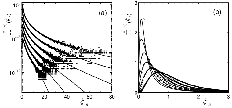
Figure 4: PDFs of Energy Dissipation Rates

In Figs. 3 and 4, displayed are PDFs of velocity fluctuations and of energy dissipation rates, respectively, extracted from the time series data Mouri04 ; Mouri05 with the help of Taylor’s frozen hypothesis on (a) log and (b) linear scale. The distances $r/\eta$ between two measuring points for PDFs of velocity fluctuations and the lengths $r/\eta$ of the region in which energy dissipation rates are averaged to produce its PDF are, from the top to bottom: 28.2, 56.4, 113, 226, 451, 903. We see from these values that the increment of the consecutive PDFs is ${\it\Delta}n=-1$. The average wind velocity in the wind tunnel is 16 m/sec. The estimated inertial range is the region $44.7<r/\eta<163$. The spatial resolution is $r_{\rm min}/\eta=14.1$, and the Kolmogorov length is estimated as $\eta=1.23\times 10^{-2}$ cm. For the theoretical PDFs of velocity fluctuations, $\mu=0.380$ ($q=0.610$), ($n$, $q^{\prime}$) = (10.1, 1.78), (9.30, 1.70), (8.30, 1.65), (7.10, 1.62), (5.90, 1.55), (4.90, 1.50), whereas for the PDFs of energy dissipation rates, $\mu=0.350$ ($q=0.574$), ($n$, $q^{\prime}$, $\theta$) = (7.60, 1.66, 1.81), (6.60, 1.20, 1.91), (5.60, 1.50, 1.77), (4.70, 1.68, 1.63), (4.20, 1.90, 1.44), (3.56, 2.30, 1.10). The values $\mu$ both of velocity fluctuations and of energy dissipation rates have been extracted following the process 1) $\sim$ 4) by adjusting the zooming increment to be ${\it\Delta}n=-1$ in the analyses of PDFs. The dependence of $n$ on $r/\eta$ for velocity fluctuations and for energy dissipation rates are, respectively, adjusted by the equations $n=-1.00\log_{2}r/\eta+15.0$ and $n=-1.00\log_{2}r/\eta+12.4$. Note that the scaling exponents with the derived $\mu$ values explain the extracted one in Fig. 2 within the error bars.

In Fig. 5, solid line represents the scaling exponents $\zeta_{m}$ derived by the new route via observed PDFs of velocity fluctuations with the help of (9). The left hand side of (9) is calculated with observed PDF data made up the lack of data for larger $x_{n}$ by the theoretical PDF $\Pi_{\phi,\mbox{S}}^{(n)}(x_{n})$. Note that, within A&A model, the difference between $\Pi_{\phi}^{(n)}(x_{n})$ and $\Pi_{\phi,\mbox{S}}^{(n)}(x_{n})$ for $x_{n}>x_{n}^{*}$ is neglected, where $x_{n}^{*}$ is the point corresponding to the connection point $\xi_{n}^{*}$. In the calculation of $\gamma_{\phi,m}^{(n)}$, only observed data is used for $\Pi_{\phi}^{(n)}(x_{n})$, since the integral in (10) stops at the upper limit $x_{n}^{*}$ which is about the order of the standard deviation. The formula for the scaling exponents (2) with $\mu=0.380$ is shown in Fig. 5 by dotted line which almost overlaps with solid line. Dashed line is the result obtained by the formula (9) without making up the lack of data for larger $x_{n}$ by the substitution of theoretical PDF $\Pi_{\phi,\mbox{S}}^{(n)}(x_{n})$.

Figure 5: The Scaling exponents via PDF

The PDFs of energy transfer rates and of energy dissipation rates measured in the DNS on $4096^{3}$ mesh size by Kaneda’s group Aoyama05 at $\mbox{R}_{\lambda}=1132$ are, successfully, analyzed by the present theoretical PDFs (6) and (7) with $\phi=3$ for energy transfer rates and by PDFs (6) and (8) with $\phi=3$ for energy dissipation rates. The observed PDFs of energy transfer rates are made symmetric by averaging the data on the left and the right hand sides. The measuring distances, $r/\eta$, for the PDFs both of transfer rates and of dissipation rates are 13.7, 78.1, 449. The inertial range is estimated as $63<r/\eta<224$, the Kolmogorov length as $\eta=5.12\times 10^{-4}$, and the Taylor micro scale as $\lambda/\eta=66.2$ Aoyama05 . For the theoretical PDFs of energy transfer rates, $\mu=0.320$ ($q=0.534$), ($n$, $q^{\prime}$) = (9.00, 1.75), (6.50, 1.70), (3.80, 1.50), whereas for the PDFs of energy dissipation rates, $\mu=0.350$ ($q=0.574$), ($n$, $q^{\prime}$, $\theta$) = (7.20, 1.60, 1.30), (4.80, 1.10, 1.70), (2.30, 1.10, 4.00). The dependence of $n$ on $r/\eta$ for energy transfer rates and energy dissipation rates are, respectively, adjusted by the equations $n=-1.04\log_{2}r/\eta+12.9$ and $n=-1.01\log_{2}r/\eta+11.2$. Note that the value of $\mu$ has been extracted by adjusting the zooming increment to be ${\it\Delta}n=-2.5$ in the analyses of PDFs.

IV Conclusions

It is shown that the formulae of PDFs within A&A model for velocity fluctuations, energy dissipation rates and energy transfer rates explain, successfully, corresponding PDFs extracted from DNSs on 2048³ and 4096³ mesh sizes, and experiments performed in a wind tunnel. It is also shown that the formulae of PDFs with appropriate zooming increment ${\it\Delta}n$ corresponding to experimental situation give a new route to obtain the scaling exponents of velocity structure function, including intermittency exponent.

Extracting $\zeta_{3{\bar{q}}}$ for $-\infty<{\bar{q}}<\infty$ through the formula $\langle|x_{n}|^{{\bar{q}}}\rangle$, given by (9) with $k=1$, out of the PDFs of energy dissipation rates ($\phi=3$), we can obtain the generalized dimension $D_{{\bar{q}}}$ through (11). It may be a direct proof of the multifractal distribution of singularities in real space. Results will be given elsewhere. Note that, for ${\bar{q}}<0$, contribution of the first term in (9) becomes conspicuous, i.e., we should subtract the contributions originated from the term violating the invariance of the scale transformation.

The authors would like to thank Dr. K. Yoshida for enlightening discussions. They are also grateful to Dr. H. Mouri and to Profs. Y. Kaneda and T. Ishihara for their kindness to provide the authors with their data prior to publication.

References

- (1) A.N. Kolmogorov, Dokl. Akad. Nauk SSSR 30, 301 (1941); ibid 31, 538 (1941).
- (2) W. Heisenberg, Proc. R. Soc. A195, 402 (1948).
- (3) see, for example, U. Frisch, Turbulence —The Legacy of A.N. Kolmogorov (Cambridge Univ. Press, Cambridge, 1995), and the references therein.
- (4) T. Arimitsu and N. Arimitsu, Phys. Rev. E 61, 3237 (2000).
- (5) T. Arimitsu and N. Arimitsu, J. Phys. A: Math. Gen. 33 L235 (2000).
- (6) T. Arimitsu and N. Arimitsu, Physica A 295, 177 (2001).
- (7) T. Arimitsu and N. Arimitsu, J. Phys.: Condens. Matter 14, 2237 (2002).
- (8) N. Arimitsu and T. Arimitsu, Europhys. Lett. 60, 60 (2002).
- (9) T. Arimitsu and N. Arimitsu, Physica D 193, 218 (2004).
- (10) T. Arimitsu and N. Arimitsu, Journal of Physics: Conference Series 7, 101 (2005).
- (11) U. Frisch, G. Parisi, Turbulence and Predictability in Geophysical Fluid Dynamics and Climate Dynamics, ed by M. Ghil, R. Benzi, G. Parisi (North-Holland, New York 1985) 84.
- (12) C. Meneveau and K. R. Sreenivasan, Nucl. Phys. B (Proc. Suppl.) 2, 49 (1987).
- (13) T. Gotoh, D. Fukayama and T. Nakano, Phys. Fluids 14, 1065 (2002).
- (14) H. Mouri, private communication (2004).
- (15) H. Mouri et al, preprint (arXiv:physics/0505203) (2005).
- (16) T. Aoyama, et al, preprint (2005).