Collective dynamics and expansion of a Bose-Einstein condensate
in a random potential

Abstract

We investigate the dynamics of a Bose-Einstein condensate in the presence of a random potential created by optical speckles. We first consider the effect of a weak disorder on the dipole and quadrupole collective oscillations, finding uncorrelated frequency shifts of the two modes with respect to the pure harmonic case. This behaviour, predicted by a sum rules approach, is confirmed by the numerical solution of the Gross-Pitaevskii equation. Then we analyze the role of disorder on the one-dimensional expansion in an optical guide, discussing possible localization effects. Our theoretical analysis provides a useful insight into the recent experiments performed at LENS [J. Lye et al., Phys. Rev. Lett. 95, 070401 (2005); C. Fort et al., cond-mat/0507144].

I Introduction

The investigation of Bose-Einstein condensates (BECs) in the presence of disorder is rapidly becoming a central topic in ultracold atom physics roth ; damski ; castin ; lye ; fort ; clement ; ertmer ; paul . Bosonic systems in disordered potentials have been extensively investigated in the recent past, both experimentally and theoretically disorder . Experiments with superfluid ⁴He in porous materials have demonstrated the suppression of superfluid transport and the critical behavior at the phase transition in presence of disorder helium . From the theoretical point of view a rich variety of phenomena is expected to occur in these systems, among which the most fascinating are Anderson localization, initially proposed in the context of electron transport in disordered solids anderson , and later predicted and observed for non-interacting wave phenomena such as light w2 ; w3 , and the quantum transition to the Bose glass phase that originates from the interplay of interactions and disorder boseglass .

The demonstrated capability of using BECs as versatile tools to revisit condensed matter physics latticereview , as for example the transition from superfluid to Mott insulator greiner , suggests that these are also promising tools to engineer disordered quantum systems roth ; damski ; castin . Recently, effects of disorder created by a laser speckle have been observed on the dynamics of a BEC, including uncorrelated shifts of the quadrupole and dipole modes lye and localization phenomena during the expansion in a one-dimensional (1D) waveguide fort ; clement . Effects of disorder have also been observed for BECs in microtraps as a consequence of intrinsic defects in the fabrication of the microchip fragmentation ; Fortagh .

In Refs. lye ; fort we have shown that the main features observed in that experiments can be explained within the Gross-Pitaevskii (GP) theory. In this paper we report a detailed analysis and discussion of the theoretical approach used, comparing the effects of different kinds of random potentials. We also make a systematic comparison with the case of a periodic lattice with spacing of the order of the length scale of disorder. This helps to discriminate the effects due to the particular realization of the random potential from those that are intimately connected to the disorder.

We show that in the presence of a weak disorder the dipole and quadrupole modes of a harmonically trapped condensate are undamped in the small amplitude regime, whereas a superfluid breakdown may occur for larger oscillations. In the first case the two modes are characterized by uncorrelated frequency shifts, both in sign and amplitude, that depend on the particular realization of the perturbing potential. The average features however do not depend crucially on the particular kind of disorder, but still evidence significant differences with the periodic case. We also show that the localization effects observed during the expansion in a 1D waveguide are mainly due to a classical trapping into single wells or between barriers of the random potential. The qualitative behavior in this case is very similar to that of a periodic system.

The paper is organized as follows: we start in Sect. II by describing the system and the various kinds of disorder considered. Then in Sect. III we discuss the effect of the random potential on the dipole and quadrupole collective oscillations of the system by means of a sum rules approach and the direct solution of the GP equation. Next, in Sect. IV we address the role of disorder on the BEC expansion in a 1D waveguide by analyzing the results of the GP calculations in terms of the quantum behaviour of a single defect (well/barrier) of the potential. A detailed description on the numerical characterization of the random potentials is reported in the Appendix.

II Description of the system

In this paper we will consider the case of an elongated condensate confined in a cylindrically symmetric harmonic potential

$$V_{ho}(r_{\perp},z)=\frac{1}{2}m\omega_{\perp}^{2}r_{\perp}+\frac{1}{2}m\omega_{z}^{2}z^{2}$$ (1)

and subjected to an additional random potential $V_{R}(z)$ along the axial direction. The latter is characterized by the correlation length $l_{c}$ and the amplitude $V_{0}$, and can be written as $V_{R}(z)=V_{0}v(z)$ with the distribution of intensities of $v(z)$ being normalized to unit standard deviation. Here we will address three kinds of disorder: two corresponding to a laser speckle potential $\pm v_{S}(z)$, where the $\pm$ indicates whether it is red or blue detuned (that is, the potential can be attractive or repulsive), and another generated by a gaussian random potential $v_{G}(z)$. A detailed description on how the potentials are constructed and characterized is reported in Appendix A.

In some cases it will also be useful to compare the effect of disorder to the case of a periodic lattice $V_{L}(z)=V_{0}v_{L}(z)$. For this purpose a suitable choice is a sinusoidal potential $v_{L}(z)=2\sqrt{2}\sin^{2}(\pi z/2l_{c})$ with intensity normalized as before and whose wavevector is chosen to match the correlation length of the random potential, as discussed in Appendix A. The typical shape of the various potentials for a correlation length $l_{c}=10\mu$m is depicted in Fig 1.

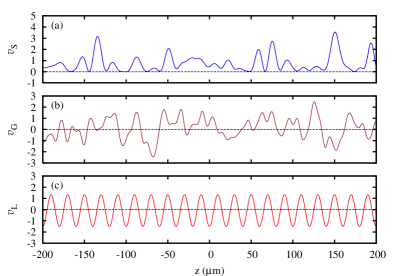
Figure 1: (Color online) Typical shape of the potentials considered in this paper: (a) (blue detuned) speckles (red speckles would have the same shape but reversed sign), (b) gaussian random, (c) periodic. In all the cases the correlation length is $l_{c}=10\mu$m.

III collective excitations

Let us start by discussing the effect of a random potential on the collective excitations of the system, considering in particular the dipole and quadrupole modes. First we will consider the regime of weak disorder and small amplitude oscillations, by comparing the prediction of sum rules with the numerical solution of the GP equation, analyzing in more details the theoretical description of the experiments reported in lye . At the end of the section we will also briefly discuss the possibility of a superfluidity breakdown that may occur for larger amplitude oscillations.

III.1 Sum rules approach

A powerful tool for characterizing the collective frequencies of the system is the sum rules approach stringari ; kimura . Within this approach an upper bound for the frequencies of the low lying collective excitations of a many-body system is given by

$$\omega^{2}=\frac{1}{\hbar^{2}}\frac{m_{3}}{m_{1}}$$ (2)

where the moments $m_{i}$ are defined via the following commutators

$$m_{1} = \langle\left[F,[H,F]\right]\rangle$$ (3)

$$m_{3} = \langle\left[[F,H],[H,[H,F]]\right]\rangle$$ (4)

between the many-body hamiltonian $H$ and a suitable excitation operator $F$ that is chosen as follows

$$F_{D} = z$$ (5)

$$F_{Q} = r_{\perp}^{2}-\alpha^{2}z^{2}$$ (6)

$\alpha$ being a variational parameter. In our case the hamiltonian can be written as

$$H=\sum_{i=1}^{N}\left[\frac{\hat{\textbf{p}}_{i}^{2}}{2m}+V_{ho}+V_{R}+g\sum_{j=1}^{i-1}\delta(\textbf{x}_{j}-\textbf{x}_{i})\right]$$ (7)

where the interaction strength $g$ is related to the interatomic scattering length $a$ by $g=4\pi\hbar^{2}a/m$, $m$ being the atomic mass.

In case of the harmonic potential $V_{ho}$ alone (unperturbed case) the dipole and quadrupole collective frequencies have the well known expressions $\omega_{D}=\omega_{z}$ for the dipole mode along $z$, and $\omega_{Q}=\sqrt{5/2}\,\omega_{z}$ for the quadrupole mode in case of an elongated condensate in the large $N$ Thomas-Fermi (TF) limit.

Let us now discuss the effect of a shallow random potential $V_{R}(z)$. Treating the $V_{R}$ as a small perturbation, and writing $\omega^{2}=\omega_{0}^{2}+\delta$ we get

$$\delta_{D} \simeq \frac{1}{m}\langle\partial_{z}^{2}V_{R}\rangle_{0}$$ (8)

$$\delta_{Q} \simeq \frac{1}{m}\frac{\langle z\partial_{z}V_{R}+z^{2}\partial_{z}^{2}V_{R}\rangle_{0}}{\langle z^{2}\rangle_{0}}$$ (9)

where the averages $\langle\cdot\cdot\rangle_{0}$ are calculated on the unperturbed ground state, and the second line is obtained assuming a strongly elongated condensate.

The above equations imply that in general the shifts of two frequencies are uncorrelated and depend on the particular shape of the perturbing potential and on its relative position respect to the harmonic potential.

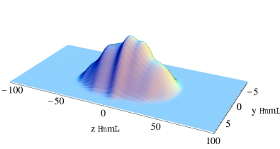
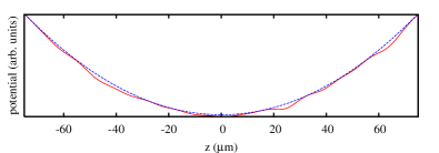
Figure 2: (Color online) (a) Column density of a typical ground state configuration in the presence of a red-detuned speckle potential ($V_{0}=2.5\,\hbar\omega_{z}$). (b) Solid line: profile of the combined potential $V_{R}$ + $V_{ho}$ (dashed line).

To show how this works in a particular example we consider here the typical parameters of the LENS experiment in lye : frequencies $\omega_{z}=2\pi\times 9$ Hz and $\omega_{\perp}=2\pi\times 90$ Hz, total number of atoms $N=1\times 10^{5}$, $V_{0}=2.5\;\hbar\omega_{z}$ and $l_{c}=10\mu$m. A picture of the total potential resulting from these parameters and of the corresponding ground state is shown in Fig. 2.

In Fig. 4 we show the frequency shifts $\Delta\omega\equiv\omega-\omega_{0}\simeq\delta/2\omega_{0}$ and their statistical distributions respectively for 100 and 1000 different realizations of the speckle potential. The picture shows that the dipole and quadrupole shifts are uncorrelated, in contrast to what happens in case of a pure harmonic potential or in the presence of a periodic potential kramer . This behavior does not depend on whether the speckles are red or blue detuned (according to Eqs. 8 and 9 this corresponds to a change of sign, and therefore the statistical properties in Fig. 4 remain unchanged). We have also verified that the behavior is essentially the same also in case of a gaussian disorder, see Fig. 4.

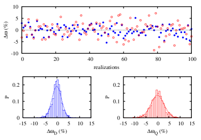
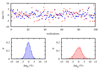
Figure 3: (Color online) Top: dipole (filled circles) and quadrupole (empty circles) frequency shifts for 100 different realizations of the speckle potential as obtained from the sum rules. Bottom: their probability distribution $P$ for 1000 realizations (left:dipole, right:quadrupole); the dashed lines are a gaussian fit.

Figure 4: (Color online) Top: dipole (filled circles) and quadrupole (empty circles) frequency shifts for 100 different realizations of the gaussian random potential as obtained from the sum rules. Bottom: their probability distribution $P$ for 1000 realizations (left:dipole, right:quadrupole); the dashed lines are a gaussian fit.

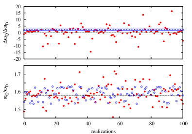
Figure 5: (Color online) Ratios between quadrupole and dipole shifts (top) and the corresponding frequencies (bottom) for speckle (filled circles) and periodic (empty circles) potentials with $l_{c}=10\mu$m. Note that although the shifts for the periodic case are correlated in sign the two frequencies are uncorrelated and depend on the actual position of the condensate in the periodic potential.

It is useful also to comment on the behaviour in the presence of a periodic potential. When the wavelength $\pi/q=2l_{c}$ of the potential is much smaller that the axial extent of the condensate one can apply the Bloch picture and resort to the effective mass approximation. As stated above, this yields the same renormalization for both the dipole and quadrupole frequencies $\omega=\sqrt{m/m^{*}}\omega_{0}$, $m^{*}$ being the effective mass kramer . Differently, in the case considered here ($l_{c}=10\mu$m) the condensate extends over only few wells of the periodic potential and the Bloch picture cannot be applied. In this case the sum rules approach predicts a sign correlated shift for the two frequencies, whose magnitude however still depends on the relative position between the condensate and the periodic potential. Therefore, although $\Delta\omega_{Q}/\Delta\omega_{D}\sim$ constant, the fact that the ratio $\omega_{Q}/\omega_{D}$ depends at first order on the difference $\Delta\omega_{Q}-\Delta\omega_{D}$ eventually yields an uncorrelated renormalization of the two frequencies (see Fig. 5).

III.2 GP dynamics

The prediction of the sum rules can be directly compared with the solution of the GP equation bec_review

$$i\hbar\partial_{t}\psi=\left[-\frac{\hbar^{2}}{2m}\nabla^{2}+V_{ho}+V_{R}+g|\psi|^{2}\right]\psi$$ (10)

by exciting the collective modes with a sudden displacement of the harmonic trap (for the dipole) or a change of the axial trapping frequency (for the quadrupole).

The results from some sample realization of the random potential are shown in Fig. 6 (they correspond to the first ten realizations in Fig. 4). The dipole oscillations are induced after a displacement $\Delta z=5\,\mu$m of the harmonic potential, corresponding to an oscillation of the order of $10\%$ of the axial size of the condensate. For the quadrupole mode, an oscillation of the same order of magnitude is obtained by releasing the condensate from a tighter trap of axial frequency $\omega_{z}^{\prime}=1.1\omega_{z}$.

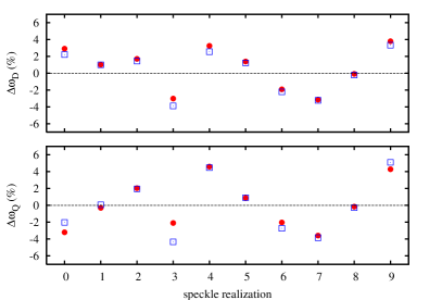
Figure 6: (Color online) Dipole (top) and quadrupole (bottom) frequency shifts as obtained from the GP equation (squares) and compared with the sum rules predictions (circles), for ten different speckle realizations. The agreement is remarkable nota1 .

In this regime of small amplitude oscillations the solution of the GP equation shows that the condensate oscillates coherently with no appreciable damping on a timescale of several oscillations. The corresponding frequencies show a remarkable agreement with the sum rules predictions, regarding both the sign and order of magnitude of the shift, as shown in Fig. 6 nota1 . As mentioned above, these features have been observed in the experiment reported in lye .

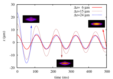
Figure 7: (Color online) Dipole oscillations in the speckle potential ($V_{0}=2.5\,\hbar\omega_{z}$) for three different displacements $\Delta z$ of the harmonic potential ($\Delta z=6,15,24\,\mu$m). The insets show a density plot for $\Delta z=24\mu$m at $t=75$ ms (left), $\Delta z=15\mu$m at $t=250$ ms (center), and $\Delta z=6\mu$m at $t=500$ ms (right).

We have also explored the behavior of the system for larger amplitudes in case of dipole oscillations, as shown in Fig. 7. As the amplitude is increased the frequency shift reduces owing to the fact that the condensate experiences outer regions of the harmonic potential where the effect of the random potential is negligible, yielding an average frequency that is closer to the unperturbed value. However, as the center of mass velocity increases, the oscillations also gets damped due to the presence of the speckle potential that acts as an external perturbation or roughness of the medium. In this regime the condensate develops short wavelength density modulation that may eventually lead to a breakdown of the superfluid flow, as shown in the left and center insets in Fig. 7 (respectively for $\Delta z=24\mu$m at $t=75$ ms and $\Delta z=15\mu$m at $t=250$ ms). The rightmost inset demonstrates instead that for small displacements the condensate remains coherent even after several oscillations ($\Delta z=6\mu$m at $t=500$ ms).

IV Expansion in a waveguide

Let us now consider the expansion of the condensate in an optical waveguide, in the presence of disorder. In this case we will refer to a second experiment performed at LENS fort . Similar experiments have also been performed by D. Clément et al. clement . The condensate is initially confined in an optical harmonic trap of frequencies $\omega_{z}=2\pi\times 30$ Hz and $\omega_{\perp}=2\pi\times 300$ Hz in the presence of a speckle potential of intensity $V_{0}=0.2~{}\mu_{TF}$, ($\mu_{TF}\simeq 87\hbar\omega_{z}$ is TF chemical potential of the condensate in the optical harmonic trap). The condensate is prepared in the ground state of the combined potential, and then let expand through the waveguide by switching off the axial trapping.

Owing to the strong radial confinement the expansion of the system can be conveniently described by the non-polynomial Schrödinger equation (NPSE) npse , that can be written in a compact form as

$$i\hbar\frac{\partial}{\partial t}\varphi=\left[-\frac{\hbar^{2}}{2m}\nabla_{z}^{2}+V(z)+\frac{\hbar\omega_{\perp}}{2}\left(3\sigma^{2}-\frac{1}{\sigma^{2}}\right)\right]\varphi$$ (11)

with $\sigma^{2}=\sqrt{1+2aN|\varphi|^{2}}$.

In Figs. 8-11 we show the density profiles of the condensate at different times during the expansion in the waveguide, for different choices of the random potential. For comparison we also show the corresponding profiles in case of a free expansion in the waveguide.

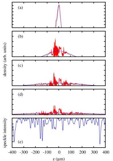
Figure 8: (Color online) (a)-(d) Density profiles of the condensate (red continuous line) during the expansion in the waveguide in the presence of a red-detuned speckle potential (shown in frame (e)), for different times ($t=0,\,25,\,50,\,75$ ms, from (a) to (d)), compared with the free expansion case (blue dashed line). Notice that the $y$-axis scale changes from (a) to (d).

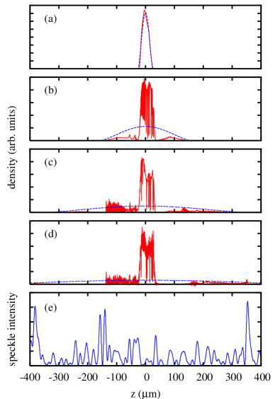
Figure 9: (Color online) (a)-(d) Density profiles of the condensate (red continuous line) during the expansion in the waveguide in the presence of a blue-detuned speckle potential (shown in frame (e)), for different times ($t=0,\,25,\,50,\,75$ ms, from (a) to (d)), compared with the free expansion case (blue dashed line). Notice that the $y$-axis scale changes from (a) to (d).

Let us discuss the figures by starting from the red-detuned speckles (the case of Ref. fort ) in Fig. 8. In this case the dynamics is characterized by an almost free expansion of the lateral wings of the condensate, whereas the central part remains localized in the deepest wells of the potential. This behavior can be easily explained by recalling that in the TF regime and in the absence of disorder the velocity field has a linear dependence on $z$, $v(z,t)=z{\dot{\lambda}_{z}(t)}/{\lambda_{z}(t)}$ ($\lambda_{z}(t)$ is a scaling parameter bec_review ), indicating that the most energetic atoms reside at the edges of the condensate whereas the atoms close to the center have a nearly vanishing velocity. The presence of a weak disorder does not modify substantially this picture. This means that the outer part of the condensate can be sufficiently energetic to pass over the defects of the potential expanding as in the unperturbed case, whereas the central part remains partially localized in the initially occupied wells (see the two density peaks in the center of the figures). A closer look to Fig. 8 shows also that in the intermediate region the density distribution shows peaks that are instead in correspondence of the maxima of the potential as a consequence of the acceleration acquired across the potential wells during the expansion.

In the presence of blue-detuned speckles, see Fig. 9, the behavior is similar although in this case the condensate may undergo a reflection from the highest barriers that eventually stop the expansion as happens at the left side of the particular disorder realization in the figure. Even in this case the central part of the condensate gets localized, being trapped by two barriers that act as a potential well in the previous case clement . We have also verified that, as one would expect, the case of a gaussian random disorder is characterized by an intermediate behavior between the former two, with part that is reflected by the highest barriers and part that is localized in the central wells.

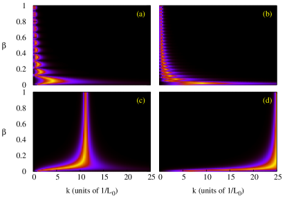
Figure 10: (Color online) Density plots of the function $q(k,\alpha,\beta)$ (see text) for a potential well ((a)-(b)) and a barrier ((c)-(d)), as a function of the incident momentum $k$ and the length scale $\beta$ of the potential. The maximum value of $k$ in the figures corresponds to an energy $E=U_{0}$. Left and right columns refer to different potential intensities: (a)-(c) $\alpha=0.2$, (b)-(d) $\alpha=1$. The plot in Figs. 8,9 must be compared with the case $\beta=1$ in (a) and (c) respectively. Dark regions indicate complete reflection or transmission, light gray (color online) corresponds to a $50\%$ transparency.

A central question is whether the observed behavior is of classical or quantum nature. Indeed, to observe non trivial localization effects caused by multiple interference of the condensate in the speckle potential, the single wells/barriers should behave as quantum reflectors nota2 . A qualitative insight on the behavior of the random potential can be therefore obtained by considering the case of a single defect. In case of the speckles a suitable model is a sech-squared potential of the form

$$U(z)=\alpha U_{0}{\rm sech}^{2}\left(\frac{z}{\beta L_{0}}\right)$$ (12)

where $\alpha$ and $\beta$ are scaling factors for energies and lengths respectively. The transmission coefficient of this potential is known analytically landau

$$T=\cases{\displaystyle\frac{\sinh^{2}(\pi\beta\tilde{k})}{\sinh^{2}(\pi\beta\tilde{k})+\cos^{2}\left(\displaystyle\frac{\pi}{2}\sqrt{1-4\alpha\beta^{2}\eta}\right)},\;4\alpha\beta^{2}\eta\leq 1\cr\cr\displaystyle\frac{\sinh^{2}(\pi\beta\tilde{k})}{\sinh^{2}(\pi\beta\tilde{k})+\cosh^{2}\left(\displaystyle\frac{\pi}{2}\sqrt{4\alpha\beta^{2}\eta-1}\right)},\,4\alpha\beta^{2}\eta>1\cr}$$ (13)

with $\eta\equiv 2mU_{0}L_{0}^{2}/\hbar^{2}$ and $\tilde{k}\equiv kL_{0}=\sqrt{2mE}L_{0}/\hbar$, $E$ being the energy of the incoming wavepacket. For convenience here we set the energy scale to the TF chemical potential of the condensate, $U_{0}=\mu_{TF}$. The length scale instead is fixed to $L_{0}=\gamma l_{c}$, with $\gamma\simeq 2.72$, in order to match, for $\beta=1$, the correlation length of the potential in Eq. (12) with that of the random potential. With this choice the correspondence with the cases shown in Figs. 8,9 is for $\alpha=0.2$ and $\beta=1$.

The ability of the above potential to act as a quantum reflector can be suitably quantified by introducing the function $q(k,\alpha,\beta)\equiv 2\,|\,0.5-T(k,\alpha,\beta)|-1$, that vanishes in case of complete transmission or reflection, and equals one for a $50\%$ transparency. In Fig. 10 we show a density plot of $q$ as a function of $k$ and $\beta$ for two values of $\alpha$, considering both the case of a potential well and of a barrier (that are relevant respectively for the comparison with the red and blue detuned speckles). The range chosen for the incident momentum $k$ corresponds to energies up to $U_{0}$. The figure shows that in case of the speckles with a correlation length as in the experiment ($\beta=1$, $\alpha=0.2$) the range of energies where quantum effects are evident is just a very narrow region close to the top of the barrier or at the well border. For this value of the correlation length even increasing the intensity of the potential (a factor of $5$ in the figure) the situation does not change substantially. Instead, by reducing the length scale of the disorder ($\beta\rightarrow 0$) quantum effects may eventually become predominant in a wide range of energies. This corresponds to the fact that the height of the single defect should vary by a quantity at least of the order of the energy $E$ of the incoming wave packet in a distance short compared to its de Broglie wavelength $\lambda_{dB}$, that is: $|dU/dz|\;\lambda_{dB}>E$. As discussed and experimentally demonstrated in fort , the above condition becomes very difficult to fulfil when the defects are created by near-infrared light as for a speckle potential.

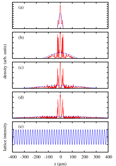
Figure 11: (Color online) (a)-(d) Density profiles of the condensate (red continuous line) during the expansion in the waveguide in the presence of a periodic lattice (shown in frame (e)), for different times ($t=0,\,25,\,50,\,75$ ms, from (a) to (d)), compared with the free expansion case (blue dashed line). Notice that the $y$-axis scale changes from (a) to (d).

These considerations suggest the interpretation of the observed localization as a classical effect due to the actual shape of the potential. In this picture the condensate gets partially localized by the presence of high barriers clement or deep wells fort in the potential that act as single traps when the local chemical potential becomes of the order of their height. This is also confirmed by the comparison with the case of the periodic potential, that presents a qualitatively similar behavior as shown in Fig. 11. Even in this case the most energetic part of the condensate expands nearly as free, whereas the bulk remains trapped in the central wells of the potential. The same picture holds even in case of a single well, as discussed in fort .

Concerning the role of interactions, we note that they introduce the dephasing at the origin of the fast density modulations shown in the figures, that may eventually lead to a breakdown of the superfluid flow as discussed in Section III.2. Their possible contribution to localization instead is not evident. Rather they act against localization, since they are responsible of the fast expansion of the lateral wings (the expansion in the noninteracting case would be much slower).

V Discussion and conclusions

A general analysis of the effects of a weak disorder created by speckle light on the collective modes and the expansion of an harmonically trapped condensate has been presented by using the Gross-Pitaevskii (GP) theory. The effects of different kinds of random potentials and a systematic comparison with the case of a periodic lattice with spacing of the order of the length scale of the disorder have been also discussed.

In the small amplitude regime the dipole and quadrupole modes are undamped and characterized by uncorrelated frequency shifts that depend on the particular realization of disorder. This behavior, predicted by a perturbative sum rules approach, has been confirmed by the direct solution of the GP equation and observed in the experiment lye . The theoretical analysis shows also that the average features do not depend crucially on the particular kind of disorder, but are however significantly different from the periodic case.

When released in a 1D waveguide the condensate may be trapped into single wells or between barriers of the random potential, yielding a reduced expansion. These phenomena are of classical nature and take place preferably near the trap center where the less energetic atoms reside. The outer part of the condensate instead expands almost freely, unless it encounters a high enough (reflecting) barrier. This behavior has been observed in recent experiments where the condensate is let expand in the presence of potential wells fort or barriers clement . In the first case the qualitative behavior is very similar to that of a periodic system or even of a single well.

We notice that in order to observe Anderson localization or related phenomena in a 1D waveguide one should instead have interference of multiple quantum reflections of matterwaves. This regime could be achieved by reducing the correlation length of the random potential, but may be not a trivial task due to the diffraction limit on the size of the defect created by light fort .

In this respect the present analysis, besides providing useful informations on the superfluid behavior of a condensate in the presence of a rough surface potential, suggests that it would be interesting to engineer other kinds of potentials by reducing the spacing or increasing the steepness.

Appendix A random distributions

In this section we discuss how the random distributions used in the paper are constructed and characterized. For simplicity here we will use dimensionless units (lengths are expressed in units of an arbitrary scale $\xi$ whose actual value is irrelevant here).

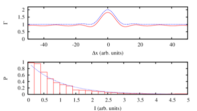
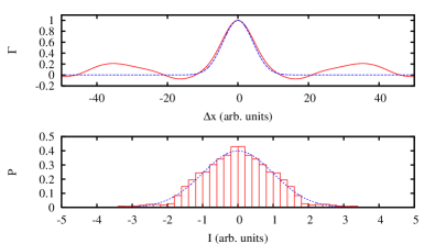
Figure 12: (Color online) Continuous line (red): autocorrelation function (top) and intensity distribution (bottom) for the speckle potential in Fig. 1. The (blue) dashed lines represent the expected average values over several realizations.

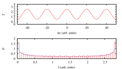
Figure 13: (Color online) Autocorrelation function (top) and intensity distribution (bottom) for the gaussian random potential in Fig. 1. The (blue) dashed lines represent the expected average values over several realizations.

Figure 14: (Color online) Autocorrelation function (top) and intensity distribution (bottom) for the periodic potential in Fig. 1.The (blue) dashed lines represent the expected average values over several realizations.

Following huntley the speckle distribution is constructed by starting from a random complex field $\varphi(x)$ (on a grid) whose real and imaginary part are obtained from two independent gaussian random distribution $\eta(x)$ with zero mean $\langle\eta(x)\rangle$=0, unit standard deviation, and correlation function $\langle\eta(x)\eta(y)\rangle\sim\delta(x-y)$. The speckle intensity field is then defined as

$$I(x)=|{\cal F}^{-1}\left[W(y){\cal F}[\varphi(x)]\right]|^{2}$$ (14)

where the operator ${\cal F}$ indicates the Fourier transform

$${\cal F}[\varphi]=\int dx\varphi(x)\textrm{e}^{2\pi ixy}$$ (15)

and $W(y)$ indicates the aperture function

$$W(y)=\cases{1&if $|y|<D/2$\cr\cr 0&elsewhere\cr}$$ (16)

The resulting distribution probability of the speckle intensities is goodman

$$P(I)=\textrm{e}^{-I/\langle I\rangle}/\langle I\rangle$$ (17)

and can be further normalized to $\sigma_{I}=\langle I\rangle\equiv 1$ (the normalized speckle distribution is indicated in the text as $v_{S}(x)$). The spatial (auto)correlation is

$$\Gamma(\Delta x)\equiv\langle I(x)I(x+\Delta x)\rangle=1+\textrm{sinc}(D\Delta x)^{2}$$ (18)

(the average $\langle\cdot\cdot\rangle$ stands for an integration over $x$ and an average over many realizations) with $\textrm{sinc}(x)\equiv\sin(\pi x)/(\pi x)$. The correlation properties can be summarized by the correlation length $l_{c}$ defined as the width at the half value of the maximum of $\Gamma(\Delta x)$ (in $\Delta x=0$) with respect to the background. In case of a one dimensional speckle distribution as that considered here $l_{c}$ is related to the aperture width by $l_{c}=0.88/D$.

As a second source of disorder we consider a gaussian random distribution defined by cheng

$$g(x)={\cal F}^{-1}\left[\sqrt{{\cal F}[W(x)]}\eta(y)\right]$$ (19)

where $\eta(y)$ itself is a gaussian random distribution (defined as above) and the aperture function is $W(x)=\exp(-x^{2}/2\sigma^{2})$. By using the properties of $\eta$ is then easy to demonstrate that both the real and imaginary part of $g(x)$ are gaussian random distributions with a correlation function $\Gamma(\Delta x)=W(\Delta x)$ and correlation length $l_{c}=2\sqrt{2\ln 2}\sigma$. Here we will consider in particular the imaginary component, $I(x)\equiv\textrm{Im}[g(x)]$ (in the text the normalized distribution is indicated as $v_{G}(x)$).

Finally let us discuss how to chose the wavevector of the periodic potential $v_{L}(x)$. In this case, the periodicity of the potential reflects in the periodic structure of the correlation function $\Gamma(\Delta x)\sim 1+2\cos^{2}(q\Delta x)$. By restricting over a single period the correlation length can be defined as above, and a straightforward calculation yields $q=\pi/2l_{c}$. A suitable choice to compare the effect of disorder to the case of an ordered lattice described by the periodic potential $v_{L}(x)$ is therefore to require the two potential to have the same correlation length. This seems a reasonable choice as shown in Fig. 1.

The autocorrelation functions and the intensity distributions of the three potentials are shown in Figs. 14-14.

References

- (1) R. Roth and K. Burnett, Phys. Rev. A 68, 023604 (2003).
- (2) B. Damski, J. Zakrzewski, L. Santos, P. Zoller, and M. Lewenstein, Phys. Rev. Lett. 91, 080403 (2003).
- (3) U. Gavish and Y. Castin, Phys. Rev. Lett. 95, 020401 (2005).
- (4) J. E. Lye, L. Fallani, M. Modugno, D. S. Wiersma, C. Fort, and M. Inguscio, Phys. Rev. Lett. 95, 070401 (2005).
- (5) D. Clément et al., cond-mat/0506638, to appear on Phys. Rev. Lett.
- (6) C. Fort, L.Fallani, V. Guarrera, J. Lye, M. Modugno, D. S. Wiersma, and M. Inguscio, cond-mat/0507144, to appear on Phys. Rev. Lett.
- (7) T. Schulte et al., cond-mat/0507453.
- (8) T. Paul et al., cond-mat/0509446.
- (9) G. E. Astrakharchik, J. Boronat, J. Casulleras, and S. Giorgini, Phys. Rev. A 66, 023603 (2002); S. Giorgini, L. Pitaevskii, S. Stringari, Phys. Rev. B 49, 12938 (1994); K. Huang and H. F. Meng, Phys. Rev. Lett. 69, 644 (1992); A. V. Lopatin and V. M. Vinokur, Phys. Rev. Lett. 88, 235503 (2002).
- (10) J. D. Reppy, J. Low Temp. Phys. 87, 205 (1992) and references therein.
- (11) P. W. Anderson, Phys. Rev. 109, 1492 (1958).
- (12) S. John, Phys. Rev. Lett. 53, 2169 (1984).
- (13) R. Dalichaouch et al., Nature 354, 53 (1991); D. S. Wiersma et al., Nature 390, 671 (1997); A. A. Chabanov and A. Z. Genack, Phys. Rev. Lett. 87, 233903 (2001).
- (14) M. P. A. Fisher, P. B. Weichman, G. Grinstein, D. S. Fisher, Phys. Rev. B 40, 546 (1989); R. T. Scalettar, G. G. Batrouni, and G. T. Zimanyi, Phys. Rev. Lett. 66, 3144 (1991); W. Krauth, N. Trivedi, and D. Ceperley, Phys. Rev. Lett. 67, 2307 (1991).
- (15) J. H. Denschlag et al., J. Phys. B 35, 3095 (2002).
- (16) M. Greiner et al., Nature 415, 39 (2002).
- (17) S. Kraft et al., J. Phys. B 35, L469 (2002); A. E. Leanhardt et al., Phys. Rev. Lett. 90, 100404 (2003); J. Estève et al., Phys. Rev. A 70, 043629 (2004); D. W. Wang, M. D. Lukin, and E. Demler, Phys. Rev. Lett. 92, 076802 (2004).
- (18) J. Fortágh, H. Ott, S. Kraft, A. Günther, and C. Zimmermann, Phys. Rev. A 66, 041604(R) (2002).
- (19) S. Stringari, Phys. Rev. Lett. 77, 2360 (1996).
- (20) T. Kimura, H. Saito, Hiroki; M. Ueda, J. Phys. Soc. Jpn., 68, 1477 (1999).
- (21) M. Krämer, L. Pitaevskii, S. Stringari, Phys. Rev. Lett. 88, 180404 (2002).
- (22) F. Dalfovo, S. Giorgini, L. P. Pitaevskii, S. Stringari, Rev. Mod. Phys. 71, 463 (1999).
- (23) Notice that the sum rules should provide an upper bound for the actual frequencies obtained from the GP equation bec_review . In our case, owing to the perturbative approach, this is true for the dipole mode but not always for the quadrupole mode.
- (24) L. Salasnich, Laser Physics 12, 198 (2002); L. Salasnich, A. Parola, and L. Reatto, Phys. Rev. A 65, 043614 (2002).
- (25) This requirement is necessary in 1D, but not in higher dimensions where interference can take place between components scattered at different angles.
- (26) L. D. Landau and E. M. Lifshitz, Quantum mechanics: non-relativistic theory, (Pergamon press, Oxford, 1977). See also: C. Lee and J. Brand, cond-mat/0505697.
- (27) J. M. Huntley, Appl. Opt. 28, 4316 (1989). P. Horak, J.-Y. Courtois, and G. Grynberg, Phys. Rev. A 58, 3953 (1998).
- (28) J. W. Goodman, Speckle Phenomena: Theory and Applications, preprint (available at http://homepage.mac.com/jwgood/Speckle_Book).
- (29) C. Cheng, C. Liu, S. Teng, N. Zhang, and M. Liu, Phys. Rev. E 65, 061104 (2002).