Parametric coupling for superconducting qubits

Abstract

We propose a scheme to couple two superconducting charge or flux qubits biased at their symmetry points with unequal energy splittings. Modulating the coupling constant between two qubits at the sum or difference of their two frequencies allows to bring them into resonance in the rotating frame. Switching on and off the modulation amounts to switching on and off the coupling which can be realized at nanosecond speed. We discuss various physical implementations of this idea, and find that our scheme can lead to rapid operation of a two-qubit gate.

The high degree of control which has been achieved on microfabricated two-level systems based on Josephson tunnel junctions qubits ; Vion02 ; Chiorescu03 has raised hope that they can form the basis for a quantum computer. Two experiments, representing the most advanced quantum operations performed in a solid-state environment up to now, have already demonstrated that superconducting qubits can be entangled Pashkin04 ; Martinis05 . Both experiments implemented a fixed coupling between two qubits, mediated by a capacitor. The fixed-coupling strategy would be difficult to scale to a large number of qubits, and it is desirable to investigate more sophisticated schemes. Ideally, a good coupling scheme should allow fast 2-qubit operations, with constants of order $100MHz$. It should be possible to switch it ON and OFF rapidly with a high ON/OFF ratio. It should also not introduce additional decoherence compared to single qubit operation. Charge and flux qubits can be biased at a symmetry point Vion02 ; Bertet04_condmat where their coherence times are the longest because they are insensitive to first order to the main noise source, charge and flux-noise respectively. It is therefore advantageous to try to keep all such quantum bits biased at this symmetry point during experiments where two or more are coupled. In that case, the resonance frequency of each qubit is set at a fixed value determined by the specific values of its parameters and can not be tuned easily. The critical currents of Josephson junctions are controlled with a typical precision of only $5\%$. The charge qubit energy splitting at the symmetry point depends linearly on the junction parameters so that it can be predicted with a similar precision. The flux-qubit energy splitting (called the gap and noted $\Delta$) on the other hand depends exponentially on the junctions critical current Orlando99 and it is to be expected that two flux-qubits with nominally identical parameters have significantly different gaps Majer04 . Therefore the problem we would like to address is the following : how can we operate a quantum gate between qubits biased at the optimal point and having unequal resonance frequencies ?

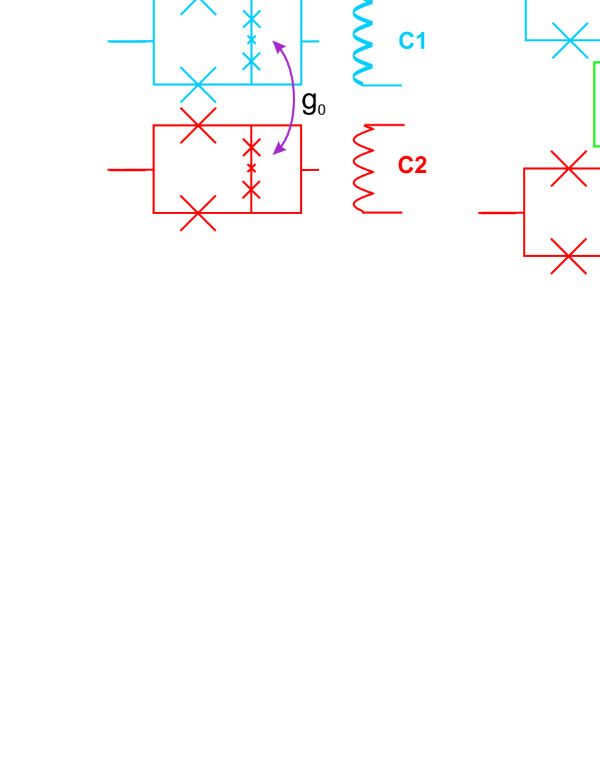
Figure 1: (Color online) a) Two flux-qubits (shown coupled to their read-out SQUIDs and to their flux control line $C_{i}$ ($i=1,2$)) coupled by a fixed mutual inductance $M$. b) Parametric coupling scheme : the two flux-qubits are now coupled through a circuit that allows to modulate the coupling constant $g$ through the control parameter $\lambda$.

We first discuss why the simplest fixed linear coupling scheme as was implemented in the two-qubit experiments Pashkin04 ; Martinis05 fails in that respect. Consider two flux qubits biased at their flux-noise insensitive point $\gamma_{Q}=\pi$ ($\gamma_{Q}$ being the total phase drop across the three junctions), and inductively coupled as shown in figure 1a Majer04 . The uncoupled energy states of each qubit are denoted $|0_{i}\rangle$,$|1_{i}\rangle$ ($i=1,2$) and their minimum energy separation $h\Delta_{i}\equiv\hbar\omega_{i}$. Throughout this article, we will suppose that $\Delta_{1}\geq\Delta_{2}$. As shown before Majer04 ; Nakamura_coupling , the system hamiltonian can be written as $H=H_{q1}+H_{q2}+H_{I}$, with $H_{qi}=-(h/2)\Delta_{i}\sigma_{zi}$ ($i=1,2$) and $H_{I}=hg_{0}\sigma_{x1}\sigma_{x2}=hg_{0}(\sigma_{1}^{+}\sigma_{2}^{+}+\sigma_{1}^{-}\sigma_{2}^{-}+\sigma_{1}^{+}\sigma_{2}^{-}+\sigma_{1}^{-}\sigma_{2}^{+})$. Here we introduced the Pauli matrices $\sigma_{x..z;i}$ referring to each qubit subspace, the raising (lowering) operators $\sigma_{i}^{+}$ ($\sigma_{i}^{-}$) and we wrote the hamiltonian in the energy basis of each qubit. It is more convenient to rewrite the previous hamiltonian in the interaction representation, resulting in $H^{\prime}_{I}=\exp(i(H_{q1}+H_{q2})t/\hbar)H_{I}\exp(-i(H_{q1}+H_{q2})t/\hbar)$. We obtain

$$\begin{array}[]{rcl}H^{\prime}_{I}&=&hg_{0}[\exp(i(\omega_{1}+\omega_{2})t)\sigma_{1}^{+}\sigma_{2}^{+}\\ &+&\exp(i(-\omega_{1}-\omega_{2})t)\sigma_{1}^{-}\sigma_{2}^{-}\\ &+&\exp(i(\omega_{1}-\omega_{2})t)\sigma_{1}^{+}\sigma_{2}^{-}\\ &+&\exp(i(-\omega_{1}+\omega_{2})t)\sigma_{1}^{-}\sigma_{2}^{+}]\end{array}$$ (1)

As soon as $|\Delta_{1}-\Delta_{2}|>g_{0}$, the corresponding evolution operator only contains rapidly rotating terms, prohibiting any transition to take place. This is a mere consequence of energy conservation : two coupled spins can exchange energy only if they are on resonance.

More elaborate coupling strategies than the fixed linear coupling have been proposed You02 ; Cosmelli04 ; Plourde04 . In these theoretical proposals, the coupling between qubits is mediated by a circuit containing Josephson junctions, so that the effective coupling constant can be tuned by varying an external parameter (such as, for instance, the flux through a SQUID loop). Nevertheless, these schemes also require the two qubits to have the same resonant frequency $\Delta_{1}=\Delta_{2}$ if they are to be operated at their optimal biasing point. If on the other hand $\Delta_{1}\neq\Delta_{2}$, only the so-called FLICFORQ scheme proposed recently by Rigeti et al. Rigeti04 to our knowledge provides a workable $2$-qubit gate. Application of strong microwave pulses at each qubit frequency $\Delta_{i}$ induces Rabi oscillations on each qubit at a frequency $\nu_{Ri}$. When the condition $\nu_{R1}+\nu_{R2}=(\Delta_{1}-\Delta_{2})$ is satisfied, the two qubits are put on resonance and they can exchange energy. It is then possible to realize any two-qubit gate by combining the entangling pulses with single-qubit rotations. Note that in order to satisfy the above resonance condition, the two qubits should still be reasonably close in energy to avoid prohibitively large driving of each qubit which could potentially excite higher energy states or uncontrolled environmental degrees of freedom. Single-qubit driving frequencies of order $250MHz$ have been achieved for charge- and flux-qubits Colin04 ; Chiorescu04 . In order to implement the FLICFORQ scheme, one would thus need the resonance frequencies of the two qubits to differ by at most $500MHz$, which seems within reach for charge-qubits but not for flux-qubits.

While in the scheme proposed by Rigeti et al. quantum gates are realized with a fixed coupling constant $g$, our scheme relies on the possibility to modulate $g$ by varying a control parameter $\lambda$. This gives us the possibility of realizing two-qubit operations with arbitrary fixed qubit frequencies, which is particularly attractive for flux-qubits. We first assume that we dispose of a “black box” circuit realizing this task, as shown in figure 1b, actual implementation will be discussed later. Our parametric coupling scheme consists in modulating $\lambda$ at a frequency $\omega/2\pi$ close to $\Delta_{1}-\Delta_{2}$ or $\Delta_{1}+\Delta_{2}$. Supposing $\lambda(t)=\lambda_{0}+\delta\lambda\cos\omega t$ leads to $g(t)=g_{0}+\delta gcos(\omega t)$, with $g_{0}=g(\lambda_{0})$ and $\delta g=(dg/d\lambda)\delta\lambda$. Then, if $\omega$ is close to the difference in qubit frequencies $\omega=\omega_{1}-\omega_{2}+\delta_{12}$ while $|\delta_{12}|<<|\omega_{1}-\omega_{2}|$, a few terms in the hamiltonian 1 will rotate slowly. Keeping only these terms, we obtain

$$\begin{array}[]{rcl}H^{\prime}_{I}&=&h(\delta g/2)(\exp(i\delta_{12}t)\sigma_{1}^{-}\sigma_{2}^{+}\\ &+&\exp(-i\delta_{12}t)\sigma_{1}^{+}\sigma_{2}^{-})\end{array}$$ (2)

Modulating the coupling constant $g$ allows therefore to compensate for the rapid rotation of the coupling terms which used to forbid transitions in the fixed coupling case, and opens the possibility to realize any two-qubit gate. For instance, in order to perform a SWAP gate, one would choose $\delta=0$ and apply a microwave pulse for a duration $\Delta t=1/(2\delta g)$. One could implement the “anti-Jaynes-Cummings” hamiltonian $H^{\prime}_{I}=h(\delta g/2)(\sigma_{1}^{-}\sigma_{2}^{-}+\sigma_{1}^{+}\sigma_{2}^{+})$ as well by applying the microwave pulse at a frequency $\omega=\omega_{1}+\omega_{2}$.

We note that a recent article also proposed to apply microwave pulses at the difference or sum frequency of two inductively coupled flux-qubits in order to generate entanglement Liu05 . However the proposed approach is ineffective if the two flux-qubits are biased at their flux-insensitive point. In our proposal, modulating the coupling constant between the two qubits instead of applying the flux pulses directly through the qubit loops overcomes this limitation.

A specific attractiveness of our scheme is that the effective coupling constant driving the quantum gates $\delta g/2$ is directly proportional to the amplitude of the microwave driving. Therefore the coupling constant can be made in principle arbitrarily large by driving the modulation strong enough, although in practice each circuit will impose a maximum amplitude modulation and modulation speed which have to be respected. This is very similar to the situation encountered in ion-trapping experiments LeibfriedRMP , and in strong contrast with the situation encountered in cavity quantum electrodynamics experiments. In the latter, the vacuum Rabi frequency, fixed by the dipole matrix element and the vacuum electric field RaimondRMP ; Blais , sets a maximum speed to any two-qubit gate mediated by the cavity. We also note that the coupling can be switched ON and OFF at nanosecond speed, as fast as the switching of Rabi pulses for single-qubit operations.

The hamiltonian (2) is only approximate because it simply omits the fixed coupling term $g_{0}\sigma_{x1}\sigma_{x2}$. In order to go beyond this approximation, we separate the time-independent and the time-dependent parts of the coupling hamiltonian by writing $H_{I}=H_{I0}+H_{I}(t)$, where $H_{I0}=g_{0}\sigma_{x1}\sigma_{x2}$, $H_{I}(t)=\delta g\cos\omega_{MW}t\sigma_{x1}\sigma_{x2}$, and $\omega_{MW}$ is the frequency of the modulation. We diagonalize $H_{q1}+H_{q2}+H_{I0}$ and rewrite $H_{I}(t)$ in the energy basis of the coupled system (dressed states basis). We go to second order of the perturbation theory and use the rotating wave approximation $H_{I0}\simeq g_{0}(\sigma_{1}^{-}\sigma_{2}^{+}+\sigma_{1}^{+}\sigma_{2}^{-})$. A complete treatment is also possible but would only make the equations more complex without modifying our conclusions. In this approximation, denoting the coupled eigenstates by $|i,j^{\prime}\rangle$ ($i,j=0,1$) and their energy by $E^{\prime}_{ij}$, we obtain that

$$\begin{array}[]{rcl}|00^{\prime}\rangle&=&|0_{1},0_{2}\rangle\\ &&E^{\prime}_{00}=-h\frac{\Delta_{1}+\Delta_{2}}{2}\\ |01^{\prime}\rangle&=&|0_{1},1_{2}\rangle-\frac{g_{0}}{\Delta_{1}-\Delta_{2}}|1_{1},0_{2}\rangle\\ &&E^{\prime}_{01}=-h(\frac{\Delta_{1}-\Delta_{2}}{2}+\frac{g_{0}^{2}}{\Delta_{1}-\Delta_{2}})\\ |10^{\prime}\rangle&=&|1_{1},0_{2}\rangle+\frac{g_{0}}{\Delta_{1}-\Delta_{2}}|0_{1},1_{2}\rangle\\ &&E^{\prime}_{10}=h(\frac{\Delta_{1}-\Delta_{2}}{2}+\frac{g_{0}^{2}}{\Delta_{1}-\Delta_{2}})\\ |11^{\prime}\rangle&=&|1_{1},1_{2}\rangle\\ &&E^{\prime}_{11}=h\frac{\Delta_{1}+\Delta_{2}}{2}\end{array}$$ (3)

The new energy states are slightly energy-shifted compared to the uncoupled ones. However, it is remarkable that this energy shift does not depend on the state of the other qubit, since for instance $E^{\prime}_{10}-E^{\prime}_{00}=E^{\prime}_{11}-E^{\prime}_{01}=h(\Delta_{1}+g_{0}^{2}/(\Delta_{1}-\Delta_{2}))\equiv h(\Delta_{1}+\delta\nu)$. This implies in particular that no conditional phase shift occurs that would lead to the creation of entanglement. We now write

$$\begin{array}[]{rcl}H_{I}(t)&=&\delta g\cos(\omega_{MW}t)\sigma_{x1}\sigma_{x2}\\ &=&\delta g\cos(\omega_{MW}t)\{[1-(\frac{g_{0}}{\Delta_{1}-\Delta_{2}})^{2}]|01^{\prime}\rangle\langle 10^{\prime}|+h.c\\ &+&2\frac{g_{0}}{\Delta_{1}-\Delta_{2}}(|10^{\prime}\rangle\langle 10^{\prime}|-|01^{\prime}\rangle\langle 01^{\prime}|)\\ &+&|00^{\prime}\rangle\langle 11^{\prime}|+|11^{\prime}\rangle\langle 00^{\prime}|\}\end{array}$$ (4)

Writing $H_{I}(t)$ in the interaction representation with respect to the dressed basis as we did earlier in the uncoupled basis shows that the presence of the coupling $g_{0}$ modifies our previous analysis as follows : 1) If one wants to drive the $|01^{\prime}\rangle\rightarrow|10^{\prime}\rangle$ transition, one needs to modulate $g$ at the frequency $(E^{\prime}_{10}-E^{\prime}_{01})/h=\Delta_{2}-\Delta_{1}+2g_{0}^{2}/(\Delta_{2}-\Delta_{1})$. 2) The effective coupling constant is then reduced by a factor $1-(g_{0}/(\Delta_{1}-\Delta_{2}))^{2}$. 3) Besides the off-diagonal coupling term, the time-dependent hamiltonian contains a longitudinal component modulated at the frequency $\omega_{MW}$. Similar terms appear in the hamiltonian of single charge- or flux-qubits driven away from their symmetry point and have little effect on the system dynamics. Driving of the $|00^{\prime}\rangle\rightarrow|11^{\prime}\rangle$ would be done in the same way as discussed earlier. We conclude that our scheme provides a workable two-qubit gate in the dressed state basis for any value of the fixed coupling $g_{0}$. However the detection process is simpler to interpret if the two-qubit energy states of $H_{I0}$ are little entangled, that is if $g_{0}<<|\Delta_{1}-\Delta_{2}|$.

One might be worried that the circuit used to modulate the coupling constant opens additional decoherence channels. We therefore need to estimate the dephasing and relaxation rates. Dephasing by 1/f noise seems the most important issue. In particular the need to use Josephson junction circuits to make the coupling tunable might be a drawback since it is well-known that they suffer from $1/f$ noise. We suppose that $\lambda=\lambda_{0}+n(t)$, where $n(t)$ is a fluctuating variable with a $1/f$ power spectrum. From equation (3) we see that the coupling hamiltonian $g\sigma_{x1}\sigma_{x2}$ gives rise to a frequency shift $\delta\nu$ of qubit $1$ resonance frequency, and $-\delta\nu$ of qubit $2$. Noise in the coupling constant thus translates into noise in the qubit energy splittings. We now compute the sensitivity coefficients $D_{\lambda,z}\equiv|\langle 00^{\prime}|\partial H/\partial\lambda|00^{\prime}\rangle-\langle 10^{\prime}|\partial H/\partial\lambda|10^{\prime}\rangle|=2\pi\partial(\delta\nu)/\partial\lambda$ of each qubit to noise in $\lambda$, using the framework and the notations established in Ithier . We obtain

$$D_{\lambda,z}=2\frac{g_{0}}{\Delta_{1}-\Delta_{2}}\frac{dg}{d\lambda}(\lambda_{0})$$ (5)

Therefore, if $g_{0}<<|\Delta_{2}-\Delta_{1}|$, it is possible to have a large value of $dg/d\lambda$ allowing rapid operation of the two-qubit gate, while keeping $D_{\lambda,z}$ small. In particular, if $g_{0}=0$, the qubit is only quadratically sensitive to noise in $\lambda$ since $D_{\lambda,z}=0$. This situation is a transposition of the optimal point concept Vion02 to the two-qubit case. Therefore our scheme provides protection against $1/f$ noise arising from the junctions in the coupling circuit, whereas if the qubits were tuned into resonance with DC pulses as proposed in You02 ; Plourde04 ; Cosmelli04 $1/f$ noise would be more harmful.

Given the form of the interaction hamiltonian, it is clear that quantum noise in the variable $\lambda$ can only induce transitions in which both qubit states are flipped at the same time, i. e. $|0_{1},0_{2}\rangle\rightarrow|1_{1},1_{2}\rangle$ or $|1_{1},0_{2}\rangle\rightarrow|0_{1},1_{2}\rangle$. The damping rates for each transition can be evaluated with the Fermi golden rule similar to the single qubit case, and will depend on the nature of the impedance implementing the coupling circuit. We discuss two different cases, one where $\lambda$ shows a flat power spectrum and one where it is peaked. If the coupling circuit acts as a resistor $R$ thermalized at a temperature $T$, the relaxation rate is

$$\Gamma_{1}=4\pi^{3}(dg/d\lambda)^{2}|h(\omega_{res})|^{2}\frac{\hbar\omega_{res}}{2\pi}[coth(\frac{\hbar\omega_{res}}{2kT})+1]R$$ (6)

where $h(\omega)=(d\lambda/dV)(\omega)$ is a transfer function relating $\lambda$ to the voltage across the coupling circuit $V$. The frequency $\omega_{res}$ refers to $2\pi(\Delta_{1}+\Delta_{2})$ or $2\pi(\Delta_{1}-\Delta_{2})$, depending on the transition considered. This rate can always be made small enough by designing the circuit in order to reduce the transfer function $|h(\omega)|$, in a similar way as the excitation circuits for single-qubit operations. In the second case we may use a harmonic oscillator with an eigenfrequency $\omega_{c}$, weakly damped at a rate $\kappa$ by coupling to a bath at temperature $T$. Now the variable $\lambda$ is an operator representing the degree of freedom of the 1D oscillator. Therefore we can write that $\lambda=\lambda_{0}(a+a^{\dagger})$. In the laboratory frame, the total hamiltonian now writes $H=H_{q1}+H_{q2}+H_{c}+H_{I}$, where $H_{c}=\hbar\omega_{c}(a^{\dagger}a)$ and $H_{I}=[g_{0}+\delta g_{0}(a+a^{\dagger})]\sigma_{x1}\sigma_{x2}$ with $\delta g_{0}=(dg/d\lambda)\lambda_{0}$. Going in the interaction representation with respect to $H_{0}=H_{q1}+H_{q2}+H_{c}$, it can be seen that the coupling contains terms rotating at $\omega_{1}\pm\omega_{2}\pm\omega_{c}$. Thus as soon as the eigenfrequency of the coupling circuit is close to $\Delta_{1}\pm\Delta_{2}$, the qubit eigenstates will be mixed with the harmonic oscillator states. This is certainly not a desirable situation if one wishes to “simply” entangle two qubits. Even if $\omega_{c}\neq\Delta_{1}\pm\Delta_{2}$, there will be a remaining damping of the qubits via the coupling circuit yielding a relaxation time of the order $[(\omega_{c}-\omega_{res})/\delta g_{0}]^{2}\kappa^{-1}$, where again $\omega_{res}$ refers to $2\pi(\Delta_{1}+\Delta_{2})$ or $2\pi(\Delta_{1}-\Delta_{2})$ depending on the transition considered. In addition, fluctuations of the photon number induced for instance by thermal fluctuations may cause dephasing Bertet05_condmat if $\hbar\omega_{c}$ is comparable to $kT$. Given all these considerations, it seems desirable that the frequency $\omega_{c}$ be as high as possible, and far away from the qubit frequencies. We note that this simple analysis would actually be valid for any control or measurement channel to which the qubit is connected, and therefore does not constitute a specific drawback of our scheme.

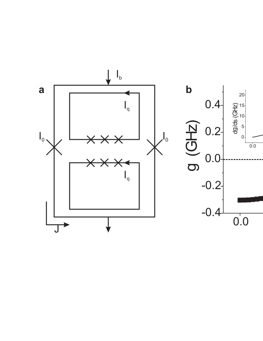
Figure 2: a) Circuit proposed in Plourde04 to implement a tunable coupling between two flux-qubits. The two qubits are directly coupled by a mutual inductance $M_{qq}$, and also via the dynamical inductance of a DC-SQUID which depends on the bias current $I_{b}$ at fixed flux bias. The total coupling constant $g$ is shown in b) for the same parameters as were considered in Plourde04 as a function of $s=I_{b}/2I_{0}$. The dashed line indicates $g=0$. Inset : (dg/ds) as a function of $s$.

We will now discuss the physical implementation of the above ideas. Simple circuits based on Josephson junctions, and thus on the same technology as the qubits themselves, allow to modulate the coupling constant at $GHz$ frequency Cosmelli04 ; Plourde04 . To be more specific in our discussion, we will focus in particular on the scheme discussed in Plourde04 , and show that the very circuit analyzed by the authors (shown in figure 2a) can be used to implement our parametric coupling scheme. Two flux-qubits of persistent currents $I_{q,i}$ and energy gaps $\Delta_{i}$ ($i=1,2$) are inductively coupled by a mutual inductance $M_{qq}$. They are also inductively coupled to a DC-SQUID with a mutual inductance $M_{qs}$. The SQUID loop (of inductance $L$) is threaded by a flux $\Phi_{S}$, and bears a circulating current $J$. The critical current of its junctions is denoted $I_{0}$. Writing the hamiltonian in the qubit energy eigenstates at the flux-insensitive point, equation (2) in Plourde04 now writes $H=-(h/2)(\Delta_{1}\sigma_{z1}+\Delta_{2}\sigma_{z2})+hg\sigma_{x1}\sigma_{x2}$, where $g=(M_{qq}|I_{q1}I_{q2}|+M_{qs}^{2}|I_{q1}I_{q2}|Re(\partial J/\partial\Phi_{s})_{I_{b}})/h$. In figure 2b we plot the coupling constant $g$ as a function of the dimensionless parameter $s=I_{b}/2I_{0}$ for the same parameters as in Plourde04 : $I_{0}=0.48\mu A$, $L=200pH$, $I_{q1}=I_{q2}=0.46\mu A$, $M_{qq}=0.25pH$, $M_{qs}=33pH$, $\Phi_{s}=0.45\Phi_{0}$. We see that $g$ strongly depends on $s$. In particular $g(s_{0})=0$ for a specific value $s_{0}$. On the other hand the derivative $dg/ds$ is finite (for instance, $dg/ds(s_{0})=7GHz$) as can be shown in the inset of figure 2b. Biasing the system at $s_{0}$ protects it against $1/f$ flux-noise in the SQUID loop and noise in the bias current. At GHz frequencies, the noise power spectrum of $s$ is ohmic due to the bias current line dissipative impedance, and has a resonance due to the plasma frequency of the SQUID junctions. This resonance is in the $40GHz$ range for typical parameters and should not affect the coupled system dynamics.

Figure 3: Calculated evolution of the density matrix under the application of an entangling microwave pulse at the frequency $|\Delta_{1}-\Delta_{2}|$ in the SQUID bias current, with $\Delta_{1}=5GHz$, $\Delta_{2}=7GHz$, $g(t)=g_{0}+\delta g\cos(2\pi(\Delta_{2}-\Delta_{1})t)$ and $\delta g=100MHz$. For the black curve, $g_{0}=0$ ; for the grey curve, $g_{0}=200MHz$.

As an example, we now describe how we would generate a maximally entangled state with two flux qubits biased at their flux-noise insensitive points, assuming $\Delta_{1}=5GHz$ and $\Delta_{2}=7GHz$. We fix the bias current in the SQUID to $I_{b}=2s_{0}I_{0}$ and start with the ground state $|0_{1},0_{2}\rangle$. We first apply a $\pi$ pulse to qubit $1$ thus preparing state $|1_{1},0_{2}\rangle$. Then we apply a pulse at a frequency $\Delta_{2}-\Delta_{1}=2GHz$ in the SQUID bias current of amplitude $\delta s=0.015$. This results in an effective coupling of strength $\delta g/2=(dg/ds)(\delta s/2)=50MHz$. A pulse of duration $\delta t=5ns$ suffices then to generate the state $(|0_{1},0_{2}\rangle+|1_{1},1_{2}\rangle)/\sqrt{2}$. We stress that thanks to the large value of the derivative $dg/ds$, even a small modulation of the bias current of $\delta I_{b}=2I_{0}\delta s=15nA$ is enough to ensure such rapid gate operation. We performed a calculation of the evolution of the whole density matrix under the complete interaction hamiltonian $g(t)\sigma_{x1}\sigma_{x2}$ with the parameters just mentioned. We initialized the two qubits in the $|1_{1},0_{2}\rangle$ state at $t=0$ ; at $t=10ns$ an entangling pulse $g(t)=\delta g\cos 2\pi(\Delta_{1}-\Delta_{2})t$ and lasting $20ns$ was simulated. The result is shown as a black curve in figure 3. We plot the diagonal elements of the total density matrix. As expected, $\rho_{00,00}(t)=\rho_{11,11}=0$, and $\rho_{10,10}=1-\rho_{01,01}=(\cos(2\pi(\delta g/2)t))^{2}$. We did another calculation for the same qubit parameters but assuming a fixed coupling $g_{0}=200MHz$. Following the analysis presented above, we initialized the system in the dressed state $|10^{\prime}\rangle$ and simulated the application of a microwave pulse $g(t)=\delta g\cos\omega_{MW}t$ at a frequency $\omega_{MW}=2.04GHz$ taking into account the energy shift of the dressed states. The evolution of the density matrix elements (grey curve in figure 3) shows that despite the finite value of $g_{0}$, the two qubits become maximally entangled as previously. The evolution is not simply sinusoidal because we plot the density matrix coefficients in the uncoupled state basis. Note also the slightly slower evolution compared to the $g_{0}=0$ case, consistent with our analysis. This shows that the scheme should actually work for a wide range of experimental parameters.

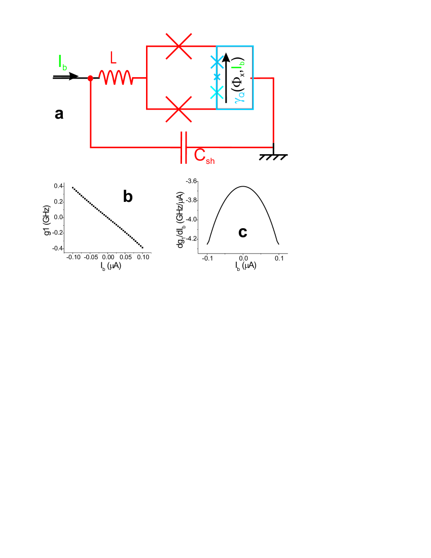
Figure 4: (Color online) Flux qubit parametrically coupled to an LC oscillator via a DC SQUID. a) Electrical scheme : the qubit (blue loop) is inductively coupled to a DC SQUID shunted by a capacitor and thus forming a LC oscillator. b) Dependence of the coupling constant $g_{1}$ as a function of the bias current $I_{b}$ Bertet05_condmat . At the current $I_{b}^{*}$ the coupling constant vanishes. c) Derivative $dg_{1}/dI_{b}$ as a function of $I_{b}$. It stays nearly at a constant value on the current range considered.

It is straightforward to extend the scheme discussed above to the case of a qubit coupled to a harmonic oscillator of widely different frequency. As an example we consider the circuit studied in Chiorescu04 ; Burkard04 ; Bertet05_condmat which is shown in figure 4a. A flux qubit is coupled to the plasma mode of its DC SQUID shunted by an on-chip capacitor $C_{sh}$ (resonance frequency $\nu_{p}$) via the SQUID circulating current $J$. As discussed in Bertet05_condmat , the coupling between the two systems can be written $H_{I}=[g_{1}(I_{b})(a+a^{\dagger})+g_{2}(I_{b})(a+a^{\dagger})^{2}]\sigma_{x}$. We evaluated $g_{1}(I_{b})$ for the following parameters : $\Phi_{S}=0.45\Phi_{0}$, $I_{0}=1\mu A$, qubit-SQUID mutual inductance $M=10pH$, qubit persistent current $I_{p}=240nA$, $\Delta=5.5GHz$, $\nu_{p}=9GHz$ as shown in figure 4b. At $I_{b}=I_{b}^{*}=0$, the coupling constant $g_{1}$ vanishes. It has been shown in Bertet05_condmat that when biased at $I_{b}=I_{b}^{*}$ and at its flux-insensitive point, the flux-qubit could reach remarkably long spin-echo times (up to $4\mu s$). On the other hand, the derivative of $g_{1}$ is shown in figure 4b to be nearly constant with a value $dg_{1}/dI_{b}\simeq-4GHz/\mu A$. Therefore, inducing a modulation of the SQUID bias current $\delta i\cos(2\pi(\nu_{p}-\Delta)t)$ with amplitude $\delta i=50nA$ would be enough to reach an effective coupling constant of $100MHz$. The state of the qubit and of the oscillator are thus swapped in $5ns$ for reasonable circuit parameters. This process is very similar to the sideband resonances which have been predicted Marlies04 and observed Chiorescu04 . However, in order to use these sideband resonances for quantum information processing, the quality factor of the harmonic oscillator must be as large as possible, contrary to the experiments described in Chiorescu04 where $Q\simeq 100$. This can be achieved by superconducting distributed resonators for which quality factors in the $10^{6}$ range have been observed Wallraff04 . Employing this harmonic oscillator as a bus allows the extension of the scheme to an arbitrary number of qubits, each of them coupled to the bus via a SQUID-based parametric coupling scheme.

In conclusion, we have presented a scheme to entangle two quantum systems of different fixed frequencies coupled by a $\sigma_{x}\sigma_{x}$ interaction. By modulating the coupling constant at the sum (difference) of their resonance frequencies, we recover a Jaynes (anti-Jaynes) -Cummings interaction hamiltonian. It also yields an intrinsic protection against 1/f noise in the coupling circuit. Our proposal is well suited for qubits based on Josephson junctions, since they readily allow tunable coupling constants to be implemented. The idea can be extended to the interaction between a qubit and a harmonic oscillator and could provide the basis for a scalable architecture for a quantum computer based on qubits, all biased at their optimal points.

We thank I. Chiorescu, A. Lupascu, B. Plourde, D. Estève, D. Vion, M. Devoret and N. Boulant for fruitful discussions. This work was supported by the Dutch Foundation for Fundamental Research on Matter (FOM), the E.U. Marie Curie and SQUBIT2 grants, and the U.S. Army Research Office.

References

- (1) Y. Nakamura, Yu. A. Pashkin, and J. S. Tsai, Nature (London) 398, 786 (1999) ; J. M. Martinis, S. Nam, J. Aumentado, and C. Urbina, Phys. Rev. Lett. 89, 117901 (2002) ; T. Duty, D. Gunnarsson, K. Bladh, P. Delsing, Phys. Rev. B 69, 140503 (2004) ; J. Claudon, F. Balestro, F. W. Hekking, O. Buisson, Phys. Rev. Lett. 93, 187003 (2004).
- (2) D. Vion, A. Aassime, A. Cottet, P. Joyez, H. Pothier, C. Urbina, D. Estève, and M. H. Devoret, Science 296, 886 (2002).
- (3) I. Chiorescu, Y. Nakamura, C. J. P. M. Harmans, and J. E. Mooij, Science 299, 1869 (2003).
- (4) Y. Pashkin et al., Nature 421, 823 (2004)
- (5) R. McDermott, R. W. Simmonds, M. Steffen, K. B. Cooper, K. Cicak, K. D. Osborn, S. Oh, D. P. Pappas, and J. M. Martinis, Science 307, 1299 (2005)
- (6) P. Bertet, I. Chiorescu, G. Burkard, K. Semba, C. J. P. M. Harmans, D.P. DiVincenzo, J. E. Mooij, Phys. Rev. Lett. 95, 257002 (2005)
- (7) J. B. Majer, F. G. Paauw, A. C. J. ter Haar, C. J. P. M. Harmans, and J. E. Mooij, Phys. Rev. Lett. 94, 090501 (2005)
- (8) J. Q. You, Y. Nakamura, and F. Nori Phys. Rev. B 71, 024532 (2005)
- (9) T. P. Orlando, J. E. Mooij, L. Tian, C. H. van der Wal, L. S. Levitov, S. Lloyd, and J. J. Mazo, Phys. Rev. B 60, 15398-15413 (1999)
- (10) J.Q. You et al., Phys. Rev. Lett. 89, 197902 (2002)
- (11) C. Cosmelli, M. G. Castellano, F. Chiarello, R. Leoni, D. Simeone, G. Torrioli, P. Carelli, cond-mat/0403690 (2004)
- (12) B. L. T. Plourde, J. Zhang, K. B. Whaley, F. K. Wilhelm, T. L. Robertson, T. Hime, S. Linzen, P. A. Reichardt, C.-E. Wu, and J. Clarke, Phys. Rev. B 70, 140501 (2004)
- (13) C. Rigetti, A. Blais, and M. Devoret, Phys. Rev. Lett. 94, 240502 (2005)
- (14) E. Collin, G. Ithier, A. Aassime, P. Joyez, D. Vion, and D. Esteve Phys. Rev. Lett. 93, 157005 (2004)
- (15) Y.-X. Liu, L.F. Wei, J.S. Tsai, and F. Nori, cond-mat/0509236 (2005)
- (16) D. Leibfried, R. Blatt, C. Monroe, D. Wineland, Rev. Mod. Phys. 75, 281 (2003)
- (17) A. Blais, R.-S. Huang, A. Wallraff, S. M. Girvin, and R. J. Schoelkopf, Phys. Rev. A 69, 062320 (2004)
- (18) J.-M. Raimond, M. Brune, S. Haroche, Review of Modern Physics 73, 565 (2003)
- (19) G. Ithier, E. Collin, P. Joyez, P. J. Meeson, D. Vion, D. Esteve, F. Chiarello, A. Shnirman, Y. Makhlin, J. Schriefl, and G. Sch n Phys. Rev. B 72, 134519 (2005)
- (20) P. Bertet, I. Chiorescu, C.J.P.M Harmans, J.E. Mooij, arXiv:cond-mat/0507290 (2005)
- (21) G. Burkard, D. P. DiVincenzo, P. Bertet, I. Chiorescu, and J. E. Mooij, Phys. Rev. B 71, 134504 (2005)
- (22) I. Chiorescu, P. Bertet, K. Semba, Y. Nakamura, C.J.P.M Harmans, and J.E. Mooij, Nature 431, 159 (2004)
- (23) A. Wallraff, D. I. Schuster, A. Blais, L. Frunzio, R.-S. Huang, J. Majer, S. Kumar, S. M. Girvin, R. J. Schoelkopf, Nature 431, 162-167 (2004)
- (24) M. C. Goorden, M. Thorwart, and M. Grifoni, Phys. Rev. Lett. 93, 267005 (2004)