Maxwell-J$\ddot{\bf u}$ttner distributions in relativistic molecular dynamics

Abstract

In relativistic kinetic theory, which underlies relativistic hydrodynamics, the molecular chaos hypothesis stands at the basis of the equilibrium Maxwell-J$\ddot{\mbox{u}}$ttner probability distribution for the four-momentum $p^{\alpha}$. We investigate the possibility of validating this hypothesis by means of microscopic relativistic dynamics. We do this by introducing a model of relativistic colliding particles, and studying its dynamics. We verify the validity of the molecular chaos hypothesis, and of the Maxwell-J$\ddot{\mbox{u}}$ttner distributions for our model. Two linear relations between temperature and average kinetic energy are obtained in classical and ultrarelativistic regimes.

I introduction

The study of relativistic fluids, both from the hydrodynamic and kinetic point of view has been widely investigated degr ; ce ; stew ; uz ; krem . In this context, the relativistic Boltzmann equation

$$p^{\,\nu}\frac{\partial f}{\partial x^{\nu}}+m_{0}\frac{\partial fF^{\nu}}{\partial p^{\,\nu}}=\int(f^{\prime}_{*}f^{\prime}-f_{*}f)\Omega\frac{d^{3}{p^{\prime}}}{{p^{\prime}}^{0}}\frac{d^{3}p_{*}}{p^{0}_{*}}\frac{d^{3}p_{*}^{\prime}}{{p^{\prime}}^{0}_{*}}\ \ ,$$ (1)

represents the best known tool, which is based on a molecular chaos hypothesis, like the Boltzmann equation in classical kinetic theory. Here $x^{\nu}$, $p^{\nu}$, $F^{\nu}$ are respectively the position, momentum and force four-vectors, $m_{0}$ is the rest mass, $\Omega$ is the interaction cross-section, and $f$ is the single particle distribution function. Collisionless relativistic plasmas are investigated by means of the relativistic Vlasov equation, obtained neglecting the collision term in Eq.(1). The equations of relativistic Hydrodynamics, which macroscopically describe relativistic fluids, are derived also from Eq.(1), similarly to the classical case.
The chaotic hypothesis, which underlies Eq.(1), explains how the microscopic components of a fluid reach a local equilibrium state. Classically, it is well established that this is a consequence of the interactions among the particles, as illustrated, for instance, by molecular dynamics aw .
In order to investigate the validity of the molecular chaos assumption in relativistic kinetic theory, we propose a simple model of $N$ relativistic colliding particles, and investigate the properties of its dynamics.
In fact, to the best of our knowledge, many particle relativistic systems have only been studied either from a kinetic or hydrodynamic point of view, because the microscopic dynamics of such particle systems presents many difficulties. For instance, it is highly problematic to write covariant hamiltonians (and the related 4-vector equations of motion) for the systems. Other difficulties concern: the choice of the reference frame, since every particle has a different proper time; the form of the interaction potential, since the action and reaction principle holds only for contact interactions; the effects of length contraction and time dilation. The consequence of this is that, as far as we know, no direct microscopic evidence for the molecular chaos hypothesis in relativistic dynamics has been provided.
To overcome this difficulty, we propose a non-covariant hamiltonian written with respect to the center of mass frame, taken as the Lorentz rest frame, which yields the non-covariant equations of motion

$$\left\{\begin{array}[]{ll}&\dfrac{d\mbox{\boldmath$x$}_{j}}{dt}=\dfrac{c\,\mbox{\boldmath$p$}_{j}}{\sqrt{\mbox{\boldmath$p$}_{j}^{2}+m_{0}^{2}c^{2}}}\\ &\\ &\dfrac{d\mbox{\boldmath$p$}_{j}}{dt}=\mbox{\boldmath$F$}_{j}^{WCA}(\mbox{\boldmath$x$})\,\,\,\,\,\,\,\,\,\,\,\,\,\ j=1,2,...,N\ \ ,\end{array}\right.$$ (5)

where $N$ is the number of particles. For the force $\mbox{\boldmath$F$}_{j}^{WCA}$ we propose to use

$$\mbox{\boldmath$F$}_{j}^{WCA}=-\sum_{i\neq j}\frac{\mbox{\boldmath$r$}_{ij}}{r_{ij}}\frac{\partial\Phi^{WCA}_{ij}}{\partial r_{ij}}=\left\{\begin{array}[]{ll}&\sum_{i\neq j}\dfrac{24\epsilon}{\sigma}\dfrac{\mbox{\boldmath$r$}_{ij}}{r_{ij}}\left[2\left(\dfrac{\sigma}{r_{ij}}\right)^{13}-\left(\dfrac{\sigma}{r_{ij}}\right)^{7}\right];\,\,\ r_{ij}<2^{1/6}\sigma\\ &0\,\,\,\,\,\,\,\,\,\,\,\,\,\,\,\,\,\,\,\,\,\,\,\,\,\,\,\,\,\,\,\,\,\,\,\,\,\,\,\,\,\,\,\,\,\,\,\,\,\,\,\,\,\,\,\,\,\,\,\,\,\,\,\,\,\,\,\,\,\,\,\,\,\,\,\,\,\,\,\,\,\,\ ;\,\,\ r_{ij}\geq 2^{1/6}\sigma\end{array}\right.$$ (8)

where $\mbox{\boldmath$r$}_{ij}=(\mbox{\boldmath$r$}_{i}-\mbox{\boldmath$r$}_{j})$, $r_{ij}=|\mbox{\boldmath$r$}_{ij}|$, $\Phi^{WCA}_{ij}$ is the Weeks-Chandler-Andersen interaction potential evmor ; the quantities $\epsilon$ and $\sigma$ are obtained from the Lennard-Jones (LJ) potential which defines $\Phi^{WCA}_{ij}$, and represent respectively the depth of the LJ potential, and the distance at which it changes sign.
Therefore, particles move according to the relativistic dynamics when they do not interact, while their interactions are modelled classically, so that the total momentum and the total kinetic energy of particles are preserved by the collision process. Although this is not completely rigorous, our procedure meets all the microscopic requirements of relativistic kinetic theory, i.e. the invariance of the momentum 4-vectors.
In this paper we simulate a 2D system of $N$ relativistic particles (with $N=28$), through a MD algorithm, which implements the equations of motion (5,8) with periodic boundary conditions, for a density $\rho=N/A=0.2$ (with $A$ the cell area), which is not a low density case. The simulations are performed for different initial kinetic energies corresponding to classical, relativistic and ultrarelativistic regimes. Furthermore, we take $\epsilon=\sigma=1$.
In the low density limit, the contribution of the collisions is expected to become negligible, and the dynamics to tend to a fully covariant dynamics.

II Results

Our results show that the simulated systems all reach an equilibrium state since their observables, such as the pressure, converge to an equilibrium value, while the probability distribution functions (PDFs) of the values of microscopic quantities like momentum $p_{x}$ and kinetic energy $\xi$ reach an invariant form. In particular, we find that the PDFs of $p_{x}$ reduce to the Maxwell-Boltzmann (MB) distribution in the classical limit, as desired. This is due to chaos in the dynamics, which is evidenced by the fact that the numerically evaluated largest Lyapounov exponents are positive.

II.1 Probability Distribution Functions

The standard relativistic kinetic theory predicts that the PDF of $p^{\alpha}$ has the form of the Maxwell-J$\ddot{\mbox{u}}$ttner (MJ) distribution, $f_{MJ}=d\exp{(-U^{\alpha}p_{\alpha}/k_{B}T)}$, with $d$ a normalization constant and $U^{\alpha}$ the hydrodynamic four-velocity (with $U^{z}=0$) degr ; ce . In the local rest frame, $f_{MJ}$ can be written as

$$f_{MJ}(p_{x},p_{y})=d\,\exp{\left(-a\sqrt{\frac{p_{x}^{2}+p_{y}^{2}}{m_{0}^{2}c^{2}}+1}\right)}\ \ ,$$ (9)

where $p_{x}$, $p_{y}$ are the spatial components of $p_{\alpha}$, $c$ is the speed of light, and where $d$ and $a$ are two constants related by the normalization condition

$$d=\left(\frac{1}{2\pi m_{0}^{2}c^{2}}\right)\frac{a^{2}e^{a}}{1+a}\ \ .$$ (10)

As well known degr ; ce , $a$ involves the temperature of the system , because

$$a=m_{0}c^{2}/k_{B}T\ \ .$$ (11)

Integrating Eq.(9) over $p_{y}$, one obtains the PDF for $p_{x}$ only:

$$g_{MJ}(p_{x})=2m_{0}cd\,\sqrt{\frac{p_{x}^{2}}{m_{0}^{2}c^{2}}+1}\,\,\cdot K_{1}\left(a\sqrt{\frac{p_{x}^{2}}{m_{0}^{2}c^{2}}+1}\right)\ \ ,$$ (12)

where $K_{1}(x)$ is the modified K-Bessel function of first order. Considering the kinetic energy $\xi=c\sqrt{\mbox{\boldmath$p$}^{2}+m_{0}^{2}c^{2}}-m_{0}c^{2}$, Eq.(9) can also be rewritten as

$$h_{MJ}(\xi)=\frac{2\pi}{c^{2}}d\,(\xi+m_{0}c^{2})\cdot\exp{\left(-a\frac{\xi+m_{0}c^{2}}{m_{0}c^{2}}\right)}\ \ .$$ (13)

It is interesting to observe that, if an expression like the MB distribution was written for the relativistic $p_{x}$, i.e. if one started from

$$f_{MB}(p_{x},p_{y})=f_{MB}(p_{x})f_{MB}(p_{y})=\frac{\tilde{a}}{\pi m_{0}^{2}c^{2}}\,\exp{\left(-\tilde{a}{\frac{p_{x}^{2}+p_{y}^{2}}{m^{2}_{0}c^{2}}}\right)}\ \ ,$$ (14)

the PDF of the relativistic kinetic energy $\xi$, after some calculations, would take the form

$$h_{MB}(\xi)=\frac{2\tilde{a}e^{\tilde{a}}}{m_{0}^{2}c^{4}}\,(\xi+m_{0}c^{2})\,\exp{\left(-\tilde{a}\frac{(\xi+m_{0}c^{2})^{2}}{m_{0}^{2}c^{4}}\right)}\ \ .$$ (15)

Comparing Eq.s ($\ref{mb},\ref{mbe}$) with Eq.s ($\ref{mjpx},\ref{mje}$), one notices that the MJ distribution is not merely the MB distribution with the relativistic $p_{x}$ and $\xi$ in place of the classical momentum and kinetic energy.
We fit the histograms constructed through our MD simulations to the PDFs given above, and for simplicity we take $m_{0}=c=1$.
The following figures are obtained for different mean kinetic energies, where the mean kinetic energy is the time average of the total kinetic energy divided by the number of particles. The histograms are constructed recording the instantaneous values of momentum $p_{x}$ and kinetic energy $\xi$ for a given particle. This operation is repeated every 200 timesteps, in order to decorrelate the recorded data.

Mean kinetic energy per particle = $9.87\times 10^{-2}$

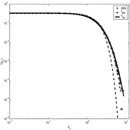
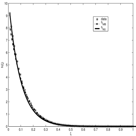
Figure 1: Fit of the data for momentum $p_{x}$ on a log scale (left panel). Fitted histograms of the kinetic energy $\xi$ in linear scale (right panel). The parameter of the Maxwell-J$\ddot{\mbox{u}}$ttner PDFs takes the value $a=10.4875$ for the PDF of$p_{x}$ yielding $k_{B}T=0.095$ (left panel), and $a=11.2595$ for the PDF of $\xi$ leading to $k_{B}T=0.089$ (right panel). The classical Maxwell Boltzmann PDFs fits well the data only in the low energy cases.

Mean kinetic energy per particle = $9.83\times 10^{-1}$

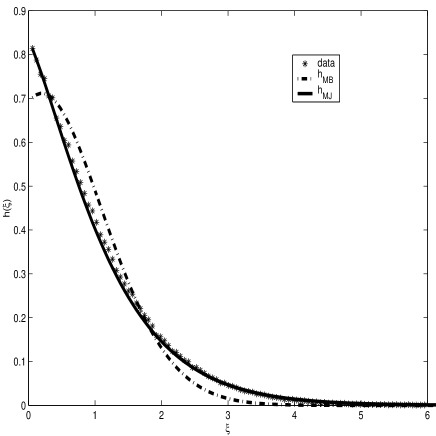
Figure 2: Fit of the data for momentum $p_{x}$ on a log scale (left panel). Fitted histograms of the kinetic energy $\xi$ in linear scale (right panel). The parameter of the Maxwell-J$\ddot{\mbox{u}}$ttner PDFs takes the value $a=1.4067$ for the PDF of $p_{x}$ yielding $k_{B}T=0.711$ (left panel), and $a=1.4225$ for the PDF of $\xi$ leading to $k_{B}T=0.703$ (right panel). The classical MJ distributions fits better the data than the MB ones at these energies.

Mean kinetic energy per particle = $6.87$

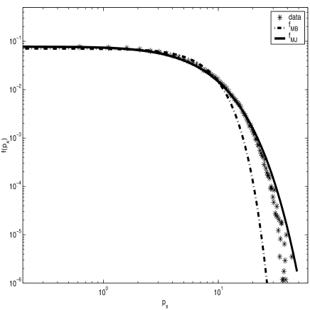
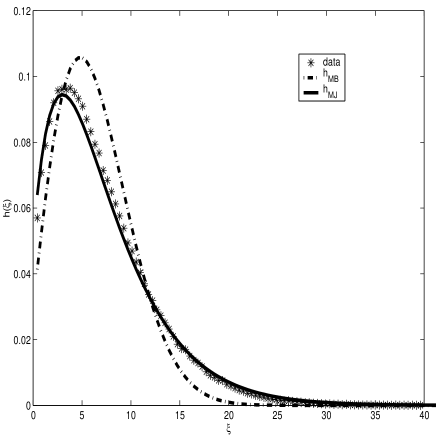
Figure 3: Fit of the data for momentum $p_{x}$ on a log scale (left panel). Fitted histograms of the kinetic energy $\xi$ in linear scale (right panel). The parameter of the Maxwell-J$\ddot{\mbox{u}}$ttner PDFs takes the value $a=0.2540$ for the PDF of $p_{x}$ yielding $k_{B}T=3.937$ (left panel), and $a=0.2501$ for the PDF of $\xi$ leading to $k_{B}T=3.998$ (right panel). The MB does not fit the data at these ultrarelativistic energies.

For the Maxwell-J$\ddot{\mbox{u}}$ttner PDFs, if the parameters $a$ and $d$ are obtained as independent parameters by fitting the numerical data to Eq.s (12,13), the normalization condition (10) both for $p_{x}$ and $\xi$ is verified. This indicates that the MJ-PDF is indeed appropriate for our data, and that the data are consistent.

II.2 Measurement of temperature for a relativistic system

The microscopic definition of the temperature of a system composed by relativistic particles is an open issue lands . However, the Maxwell-J$\ddot{\mbox{u}}$ttner PDF contains one parameter, which, in analogy with the classical Maxwell-Boltzmann PDF is identified with the quantity $k_{B}T$. Therefore, observing that the Maxwell-J$\ddot{\mbox{u}}$ttner PDFs fit well our histograms, it becomes reasonable to assume for our system $a^{-1}=k_{B}T$ as a definition of temperature obtained from the microscopic dynamics.

Temperature vs Mean kinetic energy per particle

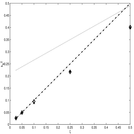
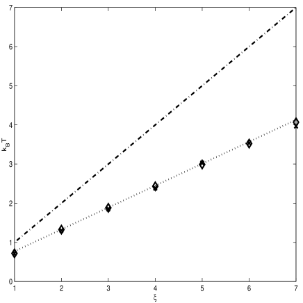
Figure 4: Plot of temperature vs mean kinetic energy per particle. Temperatures are calculated through Eq.(11) from the fitting parameter $a^{-1}=k_{B}T$, obtained both for the kinetic energy($*$) and the $p_{x}$ ($\diamond$). The two different calculations yield indistinguishable values in this figure. In the left panel the classical regime is plotted, while in the right one the ultrarelativistic limit is shown. In both panels the dotted lines represent the relation between $k_{B}$T and $\xi$ valid in the low energy cases; the dash-dotted lines the relation between $k_{B}$T and $\xi$ valid in the high energy cases.

A linear relation between this temperature and the mean value of the kinetic energy per particle has been found for the classical and ultrarelativistic cases. For $k_{B}T=a^{-1}\lesssim 0.1$ (classical regime), the relation was found to be, as expected, $k_{B}T=\xi$, while for $k_{B}T=a^{-1}\gtrsim 1$ (relativistic and ultrarelativistic regimes), we verified a linear relation of the form $k_{B}T=0.56\xi+0.21$. The transition between the two regimes takes place in a small range of kinetic energy values.

III Conclusions

In this paper we have tested a 2D molecular dynamics model intended to simulate the microscopic dynamics of $N$ relativistic colliding particles, with total constant energy $E$, and have observed its relaxation to an equilibrium state.
Our model satisfies the requirements of momentum and kinetic energy conservation before and after the collisions, underlying the equilibrium relativistic kinetic theory. The histograms found by these simulations for the momentum $p_{x}$, and for the kinetic energy $\xi$ are well fitted by the PDFs of the standard relativistic kinetic theory, i.e. by the PDFs derived from the MJ distributions. In addition to this, the statistics of the dynamics of our model reduces to the classical one when the kinetic energy takes small values.
Our model suffers from the difficulties of not being fully relativistic, because the particle interactions are treated classically; therefore, it becomes more and more acceptable as the particle density decreases, or the collision rate tends to zero making the dynamics tend to a fully covariant form. Moreover, as we are going to report in alron , reducing densities does not produce any qualitatively different result, which indicates that in the limit of low collision rates the macroscopic behaviour of our systems is not substantially different from that of the higher density cases. This, together with the observed validity of the MJ distributions, provides a justification for our model, as a tool to simulate relativistic many particle systems. Otherwise, if this model is accepted, it affords a microscopic justification of the relativistic molecular chaos hypothesis, underlying relativistic kinetic theory and relativistic hydrodynamics.
Furthermore, linear relations of temperature and mean kinetic energy have been found both in classical and ultrarelativistic regimes. This allows us to obtain a definition of temperature in a relativistic system, something rather problematic in general lands , which deserves further investigations.

References

- (1) S.R. de Groot, W.A. van Leeuwen, and Ch.G. van Weert, Relativistic Kinetic Theory North-Holland, Amsterdam , (1980)
- (2) C. Cercignani, G.M.Kremer, The Relativistic Boltzmann Equation: Theory and Application, Birkhuser Progress in mathematical Physics Vol. 22 (2000)
- (3) J.M. Stewart, Non-equilibrium relativistic kinetic theory (Lecture notes in Physics 10), Berlin:Springer, (1971)
- (4) J.P. Uzan, Dynamics of relativistic interacting gases: from a kinetic to a fluid description, Class. Quantum Grav., 15, 1063-1088, (1998)
- (5) G.M. Kremer, F.P. Devecchi, Thermodynamics and kinetic theory of relativistic gases in 2-D cosmological models, Phys.Rev. D65 083515 (2002)
- (6) B.J. Alder, T.E. Wainwright, J. Chem. Phys. 27, 1208, (1957)
- (7) D.J. Evans, G.P.Morriss, Statistical Mechanics of Nonequilibrium Liquid, Academic Press, London, Theoretical Chemistry Monograph Series, (1990)
- (8) Ingo Meller, Tommaso Ruggeri, Extended Thermodynamics, Springer Tracts in Natural Philosophy vol. 37, Springer Verlag (1993)
- (9) P.T. Landsberg, G.E.A. Matsas, Laying the ghost of the relativistic temperature transformation, Phys. Lett. A 223, 401-403, (1996)
- (10) A. Aliano, L. Rondoni, (in preparation)