Crystalline Particle Packings on a Sphere with Long Range Power Law Potentials

Abstract

The original Thomson problem of “spherical crystallography” seeks the ground state of electron shells interacting via the Coulomb potential; however one can also study crystalline ground states of particles interacting with other potentials. We focus here on long range power law interactions of the form $1/r^{\gamma}$ ($0<\gamma<2$), with the classic Thomson problem given by $\gamma=1$. At large $R/a$, where $R$ is the sphere radius and $a$ is the particle spacing, the problem can be reformulated as a continuum elastic model that depends on the Young’s modulus of particles packed in the plane and the universal (independent of the pair potential) geometrical interactions between disclination defects. The energy of the continuum model can be expressed as an expansion in powers of the total number of particles, $M\sim(R/a)^{2}$, with coefficients explicitly related to both geometric and potential-dependent terms. For icosahedral configurations of twelve 5-fold disclinations, the first non-trivial coefficient of the expansion agrees with explicit numerical evaluation for discrete particle arrangements to 4 significant digits; the discrepancy in the 5th digit arises from a contribution to the energy that is sensitive to the particular icosadeltahedral configuration and that is neglected in the continuum calculation. In the limit of a very large number of particles, an instability toward grain boundaries can be understood in terms of a “Debye–Huckel” solution, where dislocations have continuous Burgers’ vector “charges”. Discrete dislocations in grain boundaries for intermediate particle numbers are discussed as well.

I Introduction

The Thomson problem of constructing the ground state of (classical) electrons interacting with a repulsive Coulomb potential on a sphere [1] has a rich, approximately one hundred year old history [2, 3, 4]. Determining crystalline particle packings in curved geometries has a number of interesting applications in physics, mathematics, chemistry and biology particularly if one allows more general interactions amongst the particles.

An almost literal realization of the Thomson problem is provided by multi-electron bubbles [5, 6]. Electrons trapped on the surface of liquid helium by a submerged, positively charged capacitor plate have long been used to investigate two dimensional melting [7, 8]. Multi-electron bubbles result when a large number of electrons ($10^{5}{-}10^{7}$) at the helium interface subduct in response to an increase in the anode potential and coat the inside wall of a helium vapor sphere of radius $10{-}100$ microns. Typical electron spacings, both at the interface and on the sphere, are of order 2000 Angstroms, so the physics is entirely classical, in contrast to the quantum problem of electron shells which originally motivated J.J. Thomson [1]. Information about electron configurations on these bubbles can, in principle, be inferred from studying capillary wave excitations [9]. Similar electron configurations should arise on the surface of liquid metal drops confined in Paul traps [10].

A Thomson-like problem also arises in determining the arrangements of the protein subunits which comprise the shells of spherical viruses [11, 12]. Here, the “particles” are clusters of protein subunits arranged on a shell. Although the proteins interact predominantly with short range Van der Waals potentials, the same issues of spherical crystallography arise in these protein shells as in the original Thomson problem. In spherical viruses, 12 of these protein clusters sit at the vertices of a regular icosahedron in a 5-fold symmetric environment. The remaining “particles” have 6 neighboring clusters. This problem of protein arrangements was solved in a beautiful paper by Caspar and Klug [11] for intermediate values of $R/a$, where $R$ is the sphere radius and $a$ is the mean particle spacing. Caspar and Klug constructed icosadeltahedral particle packings characterized by integers $P$ and $Q$, which provide regular tessellations of

$$M=10(P^{2}+PQ+Q^{2})+2\ ,$$ (1)

protein clusters, or “particles”, on the sphere. Most known viruses (examples with $M$ as large as 1472 are known [13, 14, 15]) fall into this classification scheme, and can be studied by use of the continuum methods discussed in this paper [16]. The Caspar-Klug tessellations of the sphere provide an excellent starting point for finding low energy particle configurations on the sphere for intermediate values of $M\approx\frac{8\pi}{3}(R/a)^{2}$. Particles numbers $M$ not in the form of Eq.(1) can be accommodated by introducing vacancies or interstitials into these regular packings (see [17] for a discussion of vacancy and interstitial energies with power law potentials in flat space). New ground states involving grain boundaries are needed, however, for $M>M_{c}\approx 400-600$, and in particular in the limit $M\rightarrow\infty$ [18, 19, 20, 21, 57].

Other realizations of Thomson-like problems include regular arrangements of colloidal particles in “colloidosome” cages [22, 23, 24] proposed for protection of cells or drug-containing vesicles [25] and fullerene patterns of carbon atoms on spheres [26] and other geometries. An example with long range (logarithmic) interactions is provided by the Abrikosov lattice of vortices which would form at low temperatures in a superconducting metal shell with a large monopole at the center [27]. In practice, the “monopole” could be approximated by the tip of a long thin solenoid.

The problem of best possible packing on spheres has also applications in the micropatterning of spherical particles [28] relevant for photonic crystals or Clathrin cages, responsible for the vesicular transport of cargo in cells [29] (see [30] for a detailed theoretical study). Crystalline domains covering a fraction of the sphere are also of experimental interest. In the context of lipid rafts [31], confocal fluorescence microscopy studies have revealed the coexistence of fluid and solid domains on giant unilamellar vesicles made of lipid mixtures. The shapes of these solid domains include stripes of different widths and orientations [32, 33, 34]. The application of spherical elasticity to predict shapes of lipid mixtures domains has been discussed in [35, 36].

In the continuum approach used here, details associated with different particle interactions for the system discussed above are parameterized by a bulk and shear elastic constant and a defect core energy. In practice, defect patterns involving dislocations and disclinations depend only on the Young’s modulus and a core energy [21], which can be determined from flat particle configurations. Although we concentrate on the computationally challenging problem of long range power law potentials, explicating and complementing previous results [37], it would be straightforward to treat short range potentials as well [4].

The organization of the paper is as follows. In Sect. II, some known results for crystals on curved surfaces are reviewed and several new results are obtained. The free energy of the system is described in Sect. III. The particular case of the sphere, the Thomson problem, is discussed in Sect. IV, and several predictions for spherical lattices with icosahedral symmetry are obtained and compared with the results of direct minimizations of discrete icosadeltahedral particle arrays. The solution of the Thomson problem for a very large number of particles is discussed in Sect. V. Sect. VI contains a summary and conclusions, and some technical results are discussed in the appendices.

II Crystals of point particles

Consider a collection of classical point particles constrained to a frozen (non-dynamical) two-dimensional surface ${\cal K}$ embedded in three-dimensional Euclidean space. The particles interact through a general potential defined in the three dimensional embedding space or solely within the 2d curved surface itself. This paper focuses primarily on the potential

$$V({\vec{R}})=\frac{e^{2}}{|{\vec{R}}|^{\gamma}}\ .$$ (2)

Here, $e$ is an “electric charge” such that if $R$ is some quantity with dimensions of length,

$$e^{2}/R^{\gamma}=\mbox{dimension of energy}\ .$$

The case $\gamma=1$ corresponds to the Coulomb potential in three dimensions. Allowing we do not treat this problem explicitly here, the replacement

$$V({\vec{R}})\rightarrow\frac{e^{2}}{\gamma}(|{\vec{R}}|^{-\gamma}-1)\ ,$$ (3)

allows us to treat the two dimensional Coulomb potential by taking the limit $\gamma\rightarrow 0$,

$$V({\vec{R}})\rightarrow-e^{2}\log(|{\vec{R}}|)\ .$$ (4)

The electrostatic energy of a system of $M$ particles at positions ${\vec{R}}({\bf l})$, interacting via Eq.(2), with ${\bf l}=(l_{1},l_{2})$, $l_{1},l_{2}\in{\cal Z}$, becomes

$$2E_{0}=\sum_{{\bf l}\neq{\bf l^{\prime}}}^{M}\frac{e^{2}}{|{\vec{R}}({\bf l})-{\vec{R}}({\bf l^{\prime}})|^{\gamma}}\ .$$ (5)

Note that with this definition the power law interaction acts across a cord of the sphere, as would be the case for electron bubbles in helium. The focus of this paper is the study of crystals on curved surfaces, in particular spherical crystals. There are, however, some quantities which are insensitive to the curvature of the surface, and the simpler geometry of the plane can be used to compute them. The following two subsections hence focus on planar crystalline arrays of particles interacting via the potential Eq.(2).

II.1 Planar Crystals

The electrostatic energy Eq.(5) and the corresponding elastic tensor, from which follows the elastic constants of the system, may be explicitly computed for crystalline orderings of particles in a triangular lattice.

For any non-compact surface ${\cal K}$, like the plane, the energy Eq.(5) is divergent for all $\gamma\leq 2$. If $\gamma>0$, the divergence comes exclusively from the zero mode ${\vec{G}}=0$ associated with the thermodynamic limit of infinite system size. This term (which would be subtracted off if a uniform background charge were present) can be isolated by setting ${\vec{G}}\equiv\varepsilon\ll 1$ for this mode. The detailed calculation is somewhat involved and is given in Appendix A. The final result for the ground state energy reads

$$2E_{0} = -\frac{Me^{2}}{\Gamma(\gamma/2)}(\frac{\pi}{A_{C}})^{\frac{\gamma}{2}}\left(\frac{4}{\gamma(2-\gamma)}-\sigma(\gamma)\right)+$$

$$+ Me^{2}\frac{\pi}{A_{C}}\frac{\Gamma(1-\frac{\gamma}{2})}{\gamma/2}\lim_{{\vec{G}}\rightarrow\varepsilon}\frac{2^{2-\gamma}}{|{\vec{G}}|^{2-\gamma}}$$

$$\equiv Me^{2}\theta(\gamma){\left(\frac{4\pi}{A_{C}}\right)}^{\gamma/2}$$

$$+ Me^{2}\frac{\pi}{A_{C}}\frac{\Gamma(1-\frac{\gamma}{2})}{\gamma/2}\lim_{{\vec{G}}\rightarrow\varepsilon}\frac{2^{2-\gamma}}{|{\vec{G}}|^{2-\gamma}}\ .$$

$A_{C}$ is the area of the unit cell of the triangular Bravais lattice ($A_{C}=\frac{\sqrt{3}}{2}a^{2}$) and $\Gamma$ is the Euler Gamma function. The coefficient $\sigma$ is a sum over Misra functions, defined in Eq.(77) of Appendix B. The coefficient $\theta(\gamma)$ parameterizes the nonsingular part of the energy; its dependence on the exponent $\gamma$ is shown in Table 1. This negative quantity parameterizes the binding energy of the triangular lattice after the positive “zero mode” contribution is subtracted off. For $\gamma=1$, we have a two dimensional “jellium” model. In the problem considered in the introduction, no neutralizing background is present, and the energy is rendered finite by restricting the crystal to a compact surface, like the sphere. The maximum distance between points in the surface will then provide an infrared cut-off.

For small displacements of the particles from their equilibrium positions, one has

$$E-E_{0} = \frac{e^{2}}{2}\sum_{{\bf l}\neq{\bf l}^{\prime}}\left(\frac{1}{|{\vec{R}}({\bf l})+{\vec{u}}({\bf l})-{\vec{R}}({\bf l}^{\prime})-{\vec{u}}({\bf l}^{\prime})|^{\gamma}}\right.$$ (7)

$$- \left.\frac{1}{|{\vec{R}}({\bf l})-{\vec{R}}({\bf l}^{\prime})|^{\gamma}}\right)\ ,$$

where ${\vec{u}}({\bf l})$ is a small displacement of the particle ${\bf l}$ in the plane of the surface from its equilibrium position ${\vec{R}}({\bf l})$, and therefore a tangent vector to the surface ${\cal K}$. The elastic tensor $\Pi_{\alpha,\beta}({\bf l},{\bf l^{\prime}})$ is defined as the leading term in an expansion of Eq.(7),

$$E-E_{0}=\frac{e^{2}}{2}\sum_{{\bf l},{\bf l}^{\prime}}\Pi_{\alpha\beta}({\bf l},{\bf l}^{\prime})u_{\alpha}({\bf l})u_{\beta}({\bf l}^{\prime})\ .$$ (8)

In deriving Eq.(7), we assume a constraint of fixed area per particle, enforced by a uniform background charge density or boundary conditions. This eliminates the term linear in $u_{\alpha}({\bf l})$. The physical properties of response functions are better studied in Fourier space. The detailed calculation is given in Appendix A. The final result is

$$\Pi_{\alpha\beta}({\vec{p}}) = A_{C}\sum_{l}e^{i{\vec{p}}\cdot{\vec{R}}({\bf l})}\Pi_{\alpha\beta}({\bf l},{\bf 0})$$ (9)

$$= \frac{2^{2-\gamma}\pi}{A_{C}}\frac{\Gamma(1-\gamma/2)}{\Gamma(\gamma/2)}\frac{p_{\alpha}p_{\beta}}{|{\vec{p}}|^{2-\gamma}}+$$

$$+ \frac{\eta(\gamma)}{A_{C}^{\gamma/2}}\left[|{\vec{p}}|^{2}\delta_{\alpha\beta}+\rho(\gamma)(\delta_{\mu\alpha}\delta_{\nu\beta}+\delta_{\mu\beta}\delta_{\nu\alpha})p_{\mu}p_{\nu}\right]$$

$$+ {\cal O}(|\vec{p}|^{4}).$$

The coefficients $\eta(\gamma)$ and $\rho(\gamma)$ depend only on the potential. In Table 1, some values of the coefficients for a range of potentials with $0<\gamma<2$ are listed.

$\gamma$ $\eta$ $\rho$ $-\theta$ $\gamma$ $\eta$ $\rho$ $-\theta$ $1.875$ $0.699652$ $31$ $47.763$ $0.875$ $0.199772$ $23/9$ $3.2471$ $1.75$ $0.619256$ $15$ $22.647$ $0.75$ $0.159010$ $11/5$ $2.7138$ $1.625$ $0.544152$ $87/9$ $14.288$ $0.625$ $0.122622$ $21/11$ $2.283$ $1.5$ $0.474268$ $7$ $10.118$ $0.5$ $0.090439$ $5/3$ $1.9294$ $1.375$ $0.409548$ $27/5$ $7.625$ $0.375$ $0.062279$ $1.46154^{\ast}$ $1.6352$ $1.25$ $0.349812$ $13/3$ $5.9701$ $0.25$ $0.037955$ $9/7$ $1.3881$ $1.125$ $0.295033$ $25/7$ $4.7955$ $0.125$ $0.017265$ $43/30$ $1.1787$ $1$ $0.245065$ $3$ $3.9210$

Table 1: Coefficients of the response function Eq.(9) and the energy Eq.(II.1). Results are accurate up to six digits.The coefficient $\rho$ is a rational function of $\gamma$. In ^∗ ($\gamma=0.375$)a rational number for $\rho$ accurate to six digits could not be guessed.

II.2 Continuum free energy

When the deviations from the ground state are small, the long wavelength lattice deformations may be described by a continuous Landau elastic energy

$$F(u)=\int d^{2}{\bf r}\left[\mu u^{2}_{\alpha\beta}+\frac{\lambda}{2}u_{\alpha\alpha}^{2}\right]\ .$$ (10)

The couplings $\lambda$ and $\mu$ are the usual Lamé coefficients. The strain tensor $u_{\alpha\beta}$ is defined by

$$u_{\alpha\beta}=\frac{1}{2}(\partial_{\alpha}u_{\beta}+\partial_{\beta}u_{\alpha})\ ,$$ (11)

where ${\vec{u}}({\bf x})$ are the small displacements of Eq.(8). The elastic tensor Eq.(8), within Landau elastic theory, is then

$$e^{2}\Pi_{\alpha\beta}({\vec{p}})=A_{C}(\mu|{\vec{p}}|^{2}\delta_{\alpha\beta}+(\lambda+\mu)p_{\alpha}p_{\beta})\ .$$ (12)

A comparison with Eq.(9) immediately yields an explicit expression for the elastic constants of the crystal

$$\mu = \eta(\gamma)\frac{e^{2}}{A_{C}^{1+\gamma/2}}\ \ ,\ \ \lambda=\infty$$ (13)

$$Y = \frac{4\mu(\lambda+\mu)}{2\mu+\lambda}=4\eta(\gamma)\frac{e^{2}}{A_{C}^{1+\gamma/2}}\ ,$$ (14)

where $Y$ is Young’s modulus. The result $\lambda=\infty$ is equivalent to a divergent compressional sound velocity as ${\vec{p}}\rightarrow 0$ and for $\gamma=1$ is just a statement of the incompressibility of a two-dimensional Wigner crystal. Alternatively, we can allow for wavevector-dependent elastic constants $\mu(p)$ and $\lambda(p)$ in Eq.(12). In this case $\lambda(p)$ diverges as $p\rightarrow 0$, $\lambda(p)\approx\frac{2^{2-\gamma}\pi}{A_{C}}\frac{\Gamma(1-\gamma/2)}{\Gamma(\gamma/2)}\frac{1}{p^{2-\gamma}}$, while $\rm{lim}_{p\rightarrow 0}\mu(p)$ is given by Eq.(13).

II.3 Spherical Crystals

Spherical crystals have many properties not shared by planar ones, one of the most remarkable being that there is an excess of twelve positive (five-fold) disclinations. These disclinations repel, and the simplest spherical crystals will be those having the minimum number of defects (12) located at the vertices of an icosahedron. Triangular lattices on the sphere with an icosahedral defect pattern are classified by a pair of integers $(n,m)$, as illustrated in Fig. 1. The path from one disclination to a neighboring disclination for an $(n,m)$ icosadeltahedral lattice consists of $n$ straight steps, a subsequent $60^{\circ}$ turn, and $m$ final straight steps. The geodesic distance between nearest-neighbor disclinations on a sphere of radius $R$ is $d=R\cos^{-1}(1/\sqrt{5})$. The total number of particles $M$ on the sphere described by this $(n,m)$-lattice is given by [11]

$$M=10(n^{2}+m^{2}+nm)+2\ .$$ (15)

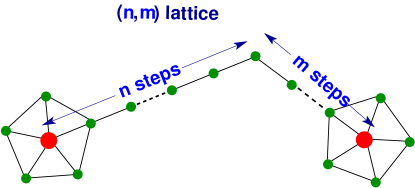
Figure 1: (Color online:)Construction of an $(n,m)$ icosadeltahedral lattice. The filled circles indicate two nearest-neighbor five fold disclinations. Because these defects sit on the vertices of an icosahedron, they are separated by a geodesic distance $R\cos^{-1}(1/\sqrt{5})$, where $R$ is the sphere radius.

.

Such $(n,m)$ configurations are believed to be ground states for relatively small numbers ($M\leq 300$, say) of particles interacting through a Coulomb potential [38, 39, 41, 42, 43]. The energy of discrete particle arrays described by Eq.(5) can be evaluated by starting with some configuration close to an $(n,m)$ one and relaxing it to find a minimum. It is found that the $(n,m)$ configurations are always local minima. Whether these icosahedral configurations are global minima as well will be analyzed later. Results for the energy E(M) are shown in the inset to Fig. 2.

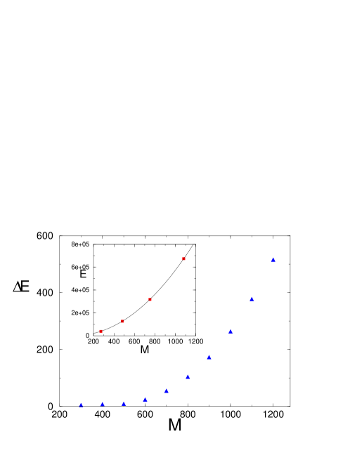
Figure 2: (Color online:)Difference in energy of $(n,n)$ and $(n,0)$ configurations. As the number of particles in the two configurations is always different (at least for relatively small n), we fitted the energy dependence on the number of particles for the two configurations, and then we computed the energy difference from the fitting curves. The energies are plotted in the inset to give an idea of the relative scale of the energy difference. Results are for a power law potential with $\gamma=1.5$ and energies are plotted in units of $\frac{e^{2}}{R^{\gamma}}$.

From Fig. 2 it is clear that energies grow very fast for increasing volume. More interestingly, the $(n,0)$ and $(n,n)$ configurations show a growing difference in energy for increasing volume size, implying that the energy of icosahedral configurations does not tend to a universal value for large numbers of particles but rather remains sensitive to the $(n,m)$ configuration, a result also noted by other authors [19, 39]. Further insight comes from investigating the distribution of energy. Plots of the local electrostatic energy, the electrostatic energy at point ${\bf x}$ on the sphere, as defined in Eq.(5) are shown in Fig. 3 [40].

Figure 3: (Color online:) Potential energy distribution for a $(n,0)$ configuration with n=10 and M=1002 (top) and a $(n,n)$ configuration with n=6 and M=1082 (bottom).

From Fig. 3 it should be noted that the triangles obtained by the Voronoi-Delaunay construction, after minimization of the potential Eq.(5), are very close to equilateral.

The distribution of the local energies for the $(n,0)$ and $(n,n)$ configurations are very different. The $(n,0)$ configuration shows maximum energies along the paths joining the defects. The $(n,n)$ configuration, on the other hand, has its maximum energies along the directions defined by the triangles formed by three nearest neighbor disclinations. The size of these regions of differing electrostatic energy turns out to scale with system size, making it very plausible that there might be small differences in the energy per particle for $(n,0)$ and $(n,n)$ configurations in the limit $n\rightarrow\infty$. This point will be discussed in more detail in coming sections.

III The Geometric Approach

The minimization of functional forms like Eq.(5) is hampered by the computational complexity of the problem, which is exponential in the particle number for spherical crystals [41]. This difficulty, which is made worse by the “geometric frustration” associated with packing particles on the sphere, limits direct approaches to minimizing the energy to systems having a small number of particles, even if much larger computer resources become available.

One way to overcome these difficulties is to substantially reduce the number of degrees of freedom that need to be considered. An approach focusing on the topological defects as degrees of freedom, rather than on the actual particles, was proposed in Refs.[21, 45]. Some aspects of this formalism are now described. The conceptual issues and developments presented in this section are applicable to crystals in any topography. Some of the results given here have already appeared in brief form in Ref.[37].

III.1 Effective free energy

The elastic energy of a curved crystal may be obtained by writing in a parametrization-invariant way the results for a flat crystal. If the metric of the curved surface is $g_{\alpha\beta}$ (with determinant $g$), the energy reads

$${\cal H}/T=E_{0}+\frac{Y}{8}(\rho|\frac{1}{\Delta^{2}}\rho)+\frac{K_{A}}{2}(\rho|\frac{1}{\Delta}\rho)+E_{s}a^{2}(s|s)\ ,$$ (16)

where $E_{0}$ is the energy of a defect-free monolayer, $(A|B)=\int d^{2}{\bf x}\sqrt{g}AB$, $\rho({\bf x})=K({\bf x})-s({\bf x})$ with $K({\bf x})$ the Gaussian curvature and $s({\bf x})$ the disclination density $s({\bf x})=\frac{\pi}{3\sqrt{g}}\sum_{i=1}q_{i}\delta({\bf x}-{\bf x}_{i})$. Here $Y$ is a Young’s modulus and $K_{A}$ is a hexatic stiffness constant. We have added a core energy term to account for the short-distance physics of disclination defects. The quantity $\frac{1}{\Delta^{2}}\rho({\bf x})$ has the meaning

$$\frac{1}{\Delta^{2}}\rho({\bf x})=\int d^{2}{\bf x}\sqrt{g}\bigl{(}\frac{1}{\Delta^{2}}\bigr{)}_{{\bf x},{\bf x^{\prime}}}\rho({\bf x^{\prime}})\,.$$ (17)

A similar expression can be defined for $\frac{1}{\Delta}\rho({\bf x})=\frac{1}{\nabla^{2}}\rho({\bf x})$. Here, $G({\bf x},{\bf x^{\prime}})\equiv\bigl{(}\frac{1}{\Delta^{2}}\bigr{)}_{{\bf x},{\bf x^{\prime}}}$ is a shorthand notation for a Green’s function which obeys $\nabla^{2}G({\bf x},{\bf x}^{\prime})=\sqrt{g}\delta({\bf x}-{\bf x}^{\prime})$, where $\nabla^{2}$ is the covariant Laplacian. Positive/negative disclinations are attracted to positive/negative curvature regions respectively. We note that at finite temperature, an additional term proportional to

$$(K|\frac{1}{\Delta}K)\ ,$$ (18)

arises from the short distance behavior of the measure (the Liouville anomaly) [46]. This term can be safely ignored in the present analysis which focuses on zero temperature.

The defect part of the free energy Eq.(16) will be used in a simplified form in the crystalline phase. In that phase the hexatic term can be incorporated into a core energy contribution proportional to the total number of defects. The energy we need to minimize becomes

$$E=E_{0}+\frac{Y}{8}(\rho|\frac{1}{\Delta^{2}}\rho)+NE_{c}\ ,$$ (19)

where $N$ is the total number of disclinations of core energy $E_{c}$.

If the disclination density were continuous, instead of being composed of discrete objects, configurations of defects such that

$$\rho=0\Rightarrow s({\bf x})=K({\bf x})\ ,$$ (20)

would be absolute minima of the free energy Eq.(19). In general, defects tend to arrange themselves on curved surfaces to screen the Gaussian curvature as efficiently as possible consistent with their discrete topological charges.

The free energy just discussed can also be applied to fluctuating geometries, as in the case of fluid or hexatic membranes (see [49, 50, 51, 52] for reviews). If Young’s modulus vanishes, corresponding to a proliferation of unbound dislocations, one obtains the free energy of an hexatic membrane [54, 46].

IV Geometric Formalism on the Sphere

Spherical substrates provide the simplest example of the problem of crystals on curved surfaces. The study of spherical crystals is simplified by two important properties: there is a unique scale with dimensions of length, the radius $R$, and there is a fixed excess disclinicity of twelve following from the Gauss-Bonnet theorem

$$\int d^{2}{\bf x}\sqrt{g({\bf x})}s({\bf x})=4\pi\rightarrow\sum_{i=1}^{N}q_{i}=12\ .$$ (21)

The free energy Eq.(19), applied to the sphere, is tractable analytically because the inverse square-Laplacian operator on a sphere of radius $R$ can be computed explicitly. It is shown in [21] that the Green’s function for the square Laplacian, in spherical coordinates $(\theta,\phi)$, has the following simple form on a unit sphere:

$$\chi(\theta^{a},\phi^{a};\theta^{b},\phi^{b})=1+\int^{\frac{1-cos\beta}{2}}_{0}dz\,\frac{\ln z}{1-z}\ ,$$ (22)

where $\beta$ is the geodesic distance between two disclinations located at $(\theta^{a},\phi^{a})$ and $(\theta^{b},\phi^{b})$,

$$\cos\beta=\cos\theta^{a}\cos\theta^{b}+\sin\theta^{a}\sin\theta^{b}\cos(\phi^{a}-\phi^{b})\ .$$ (23)

The total energy of a spherical crystal with an arbitrary number of disclinations follows from Eq.(19) and Eq.(22) and has the simple form [21]

$$2E(Y)=E_{0}+\frac{\pi Y}{36}R^{2}\sum_{i=1}^{N}\sum_{j=1}^{N}q_{i}q_{j}\chi(\theta^{i},\phi^{i};\theta^{j},\phi^{j})+N\,E_{c}\ ,$$ (24)

where $\{\theta_{i},\phi_{i}\}_{i=1,\cdots,N}$ are the coordinates of $N$ defects and we restrict ourselves to 5-fold ($q_{i}=+1$)and 7-fold ($q_{i}=-1$) defects. The quantity $E_{0}$ is the zero point energy and is defined in Eq. (II.1). Although $5$ and $7$-fold disclinations will in general have different core energies [56], we assume equal core energies here for simplicity. What matters for our calculations in any case is the dislocation core energy $E_{d}$, which we take to be $E_{d}=E_{5}+E_{7}\equiv 2E_{c}$.

The value of the Young’s modulus and the flat space ground state energy $E_{0}$ have been computed in Sect. II.1. When the sphere radius $R$ is large compared to the particle spacing $a$, we can use flat space values of $Y$ and the flat space energy $E_{0}(M)$ associated with a finite number of particles $M$. To obtain the leading terms in the expansion of the ground state energy for large but finite $M$, the precise compactification of the plane employed is irrelevant – it may be achieved by periodic boundary conditions, for example. For a sufficiently large plane the finite size effects will be negligible. The density $\sigma$ of particles is then $M$ divided by the total surface of the compact plane, taken to be the surface area of the sphere of radius $R$,

$$\sigma=1/A_{C}=\frac{M}{S}\ ,\ S=4\pi R^{2}\ .$$ (25)

From Eq.(13) the expression for the Young’s modulus suitable for $M$ particles on a spherical crystal of radius $R$ with $0<\gamma<2$ is then

$$Y=4\mu=\frac{4\eta(\gamma)M^{1+\gamma/2}}{(4\pi)^{1+\gamma/2}}\frac{e^{2}}{R^{2+\gamma}}\ .$$ (26)

One remaining detail is the divergent contribution to the energy $E_{0}$ in Eq.(II.1). Since the divergent part comes solely from the zero mode, the spatial variations in the density of the actual distribution are irrelevant. It may therefore be computed for a uniform density of charges. The divergent part is identical to the energy of a constant continuum of charges as described by the density Eq.(25). We now evaluate this divergent part of the energy on a sphere, instead of a plane.

$$E_{D} \equiv Me^{2}\frac{\pi}{A_{C}}\frac{\Gamma(1-\frac{\gamma}{2})}{\gamma/2}\lim_{\vec{G}\rightarrow\varepsilon}\frac{2^{2-\gamma}}{|\vec{G}|^{2-\gamma}}$$

$$\rightarrow \int\sqrt{g}({\bf x})\rho({\bf x})\frac{e^{2}}{|{\bf x}-{\bf x}^{\prime}|^{\gamma}}\rho({\bf x^{\prime}})\sqrt{g}({\bf x}^{\prime})$$

$$= \frac{M^{2}}{2^{\gamma-1}(2-\gamma)}\frac{e^{2}}{R^{\gamma}}\ .$$

The divergent part has thus been regularized, and the energy is finite and well-defined for all $M<\infty$.

Note that for the case $\gamma<2$ of primary interest to us here, $E_{D}\sim M^{2-\gamma/2}(M/S)^{\gamma/2}$. Hence $E_{D}$ is not simply a function of the particle density $M/S$, as one would expect for a short range interaction.

IV.1 The Energy of Spherical Crystals

Upon substituting the elastic constant of Eq.(26) into Eq.(24), one arrives at

$$2E = E_{0}+\frac{\pi Y}{36}R^{2}\sum_{i=1}^{N}\sum_{j=1}^{N}q_{i}q_{j}\chi(\theta^{i},\varphi^{i};\theta^{j},\varphi^{j})+NE_{c}$$

$$= E_{0}+\frac{4\eta(\gamma)}{(4\pi)^{1+\gamma/2}}\frac{\pi}{36}C(i_{1}\cdots i_{N})M^{1+\gamma/2}\frac{e^{2}}{R^{\gamma}}+NE_{c}\ ,$$

where $E_{0}$ is defined in Eq. (II.1) and the function $C(i_{1}\cdots i_{N})$ depends on the position $i_{1}=(\theta_{1},\phi_{1})$ etc. of the $N$ disclination charges and is universal with respect to the potential. The total energy of a spherical crystal, including the contributions to $E_{0}$ is then

$$2E_{TOT}(M) = \left(\frac{M^{2}}{2^{\gamma-1}(2-\gamma)}\right.+\Biggl{[}\frac{\theta(\gamma)}{(4\pi)^{\gamma/2}}+$$ (29)

$$\left.\frac{4\eta(\gamma)}{({4\pi})^{1+\gamma/2}}\frac{\pi}{36}C(i_{1},\cdots,i_{N})\Biggr{]}M^{1+\gamma/2}\right)\frac{e^{2}}{R^{\gamma}}$$

$$+ NE_{c}\ .$$

Note that the leading correction to the zero mode energy proportional to $M^{2}$ varies as $M^{1+\gamma/2}$, and depends both on the flat space function $\theta(\gamma)$ and on the $C$-coefficient

$$C(i_{1},\cdots,i_{N})=\sum_{j=1}^{N}\sum_{i=1}^{N}q_{i}q_{j}\chi(\theta^{i},\psi^{i};\theta^{j},\psi^{j})\ ,$$ (30)

associated with a particular configuration of disclinations.

Note that the core energies contribute to the second sub-leading coefficient. For short-range potentials, such as $\gamma>2$, the ground energy is extensive, and the leading term varies as $M^{1+\gamma/2}$.

The extensive nature of the $M^{1+\gamma/2}$ term becomes clear upon noting that

$$M^{1+\gamma/2}\frac{e^{2}}{R^{\gamma}}\propto R^{2}\times\frac{e^{2}}{a^{\gamma+2}}\ ,$$ (31)

where $a$ is the particle spacing. Comparison with Eq.(24) shows that the dimension of Young’s modulus $Y$ arises solely from the lattice constant $a$ and the electric charge $e$, consistent with elastic constants arising from physics on the scale of the lattice constant in an essentially flat geometry. This observation is now generalized to the rest of the couplings discussed in the previous section.

For the hexatic term, in Eq.(16), we have

$$\frac{K_{A}}{2}(\rho|\frac{1}{\Delta}\rho)\sim K_{A}R^{0}\sim\frac{e^{2}}{a^{\gamma}}\sim M^{\gamma/2}\frac{e^{2}}{R^{\gamma}}\ .$$ (32)

Since core energies arise as short-distance divergence’s similar to the hexatic term, they are a sub-leading contribution. For a fluid membrane not on a frozen topography, Helfrich terms arising from the extrinsic curvature $\vec{H({\bf x})}$ as well as the Gaussian curvature can be important. These scale in a way similar to the hexatic term,

$$\kappa\int d{\bf x}\sqrt{g}{\vec{H}}^{2} \sim \kappa\int d{\bf x}\sqrt{g}\frac{1}{R^{2}}\equiv\kappa R^{0}\sim M^{\gamma/2}\frac{e^{2}}{R^{\gamma}}\ ,$$

$$\kappa_{G}\int d{\bf x}\sqrt{g}K({\bf x}) \sim \kappa\int d{\bf x}\sqrt{g}\frac{1}{R^{2}}\equiv\kappa R^{0}\sim M^{\gamma/2}\frac{e^{2}}{R^{\gamma}}$$ (33)

.

Both terms would therefore contribute to the same order in the $M$ expansion as the hexatic term, although the last term is purely topological. For crystals embedded in a frozen topography we expect an expansion along the lines of Eq.(29),

$$2E_{TOT}(M)=\left(a_{0}M^{2}-\sum_{i=1}a_{i}M^{\gamma/2+1-i}\right)\frac{e^{2}}{R^{\gamma}}\ .$$ (34)

The nonextensive term $a_{0}M^{2}$ arises from the long range interactions. The next extensive contribution comes from the interaction between Gaussian curvature and defects as well as the extensive energy per particle in flat space. Hexatic terms and bending rigidity contributions are higher order in $1/M$ and can be absorbed into a redefinition of the disclination core energy. Core energies also depend on non-universal details of the short-distance physics. Core energies are included explicitly in Eqs.(19) and (29).

The results presented so far are strictly for systems at zero temperature. In systems with short range interactions, the elastic constants can be strongly temperature-dependent. An extreme example is hard disks of radius $a_{0}$, which may be viewed as a limiting case of a power law potential of the form $V(r)\simeq\epsilon_{0}\left(a_{0}/r\right)^{\gamma}$, with $\gamma\rightarrow\infty$. In this case, the elastic constants are strictly proportional to temperature. It is straightforward, however, to adapt the techniques of this paper to the simpler problem of short range pair potentials.

Figure 4: (Color Online:) Illustration of the calculation done in the text. The energy of the discrete $(n,n)$ configuration on the left is extrapolated for large $M$ and compared to the energy computed with the continuum model on the right. While in the continuum model only twelve degrees of freedom (the 12 disclinations) need to be considered, the direct calculation of a family of discrete models requires the consideration of the full lattice and a careful extrapolation of the energies to large $M$.

IV.2 Energies of Icosahedral configurations

The configuration on a sphere with the minimum number of charge $\pm 1$ defects is twelve $+1$ (5-valent) disclinations, which minimize their energy by sitting at the vertices of an icosahedron ${\cal Y}$. The energies of such configurations will be computed for the discrete spherical tessellations described in Sect. II.3 and compared with the predictions of continuum elastic theory, as illustrated in Fig. 4. It is well established that for sufficiently large values of $M$ configurations with more than 12 disclinations (i.e., those with “grain boundary scars”) have lower energies [18, 19, 21]. It is of interest, however, to study simple icosahedral configurations for large $M$, as metastable states with a well defined energy.

Within the continuum elastic theory it can be shown that twelve disclinations at the vertices of an icosahedron minimize the energy [21] when no further defects are allowed. The $C$-coefficient of Eq.(29) for this configuration of defects has been computed in [21]

$$C({\cal Y})=0.6043\ .$$ (35)

${\cal Y}$ here stands for a particle configuration with 12 defects at the vertices of an icosahedron. Using the energy of Eq.(29), the coefficient $a_{1}(\gamma,{\cal Y})$ appearing in the expansion of Eq.(34) may be computed, with the results shown in Fig. 5 and Table 2.

Figure 5: (Color online:) Energy coefficient $a_{1}$ as a function of gamma (solid line) and from the numerical results with $(n,m)$ configurations (filled circles), for the icosahedral configurations. Plot of $a_{1}(\gamma,{\cal Y})$ - $a_{1}(\gamma,{\cal Y})^{(n,n)}$ (circles), $a_{1}(\gamma,{\cal Y})$ - $a_{1}(\gamma,{\cal Y})^{(n,0)}$ (diamonds), $a_{1}(\gamma,{\cal Y})^{(n,n)}$ - $a_{1}(\gamma,{\cal Y})^{(n,0)}$ (squares).

From the results described in Sect. II.3, the $a_{1}$ coefficient may be extrapolated to very large numbers of particles using the expansion derived from Eq.(34). Indeed, as shown in Fig. 6, plots of

$$\epsilon(M)\equiv\frac{2R^{\gamma}E_{TOT}(M)/e^{2}-a_{0}(\gamma)M^{2}}{M^{1+\gamma/2}}$$ (36)

vs $1/M$ are linear, with a slope that determines $a_{1}(\gamma)$ and an intercept related to the higher order core energy-like contribution. The results of these extrapolations are shown in Table 2. The agreement between the continuum elastic theory and the explicit computation for the $(n,n)$ configuration is remarkable, holding to almost five significant figures. For the $(n,0)$ lattice there is agreement to four significant figures. This agreement is even more striking when it is recalled that the $a_{1}$-coefficient is obtained after subtraction of the term $a_{0}(\gamma)M^{2}$, as illustrated in Fig. 2. Furthermore, in the range from $\gamma=0.125$ to $\gamma=1.875$, all the significant digits vary and yet the accuracy of the calculation is virtually independent of $\gamma$.

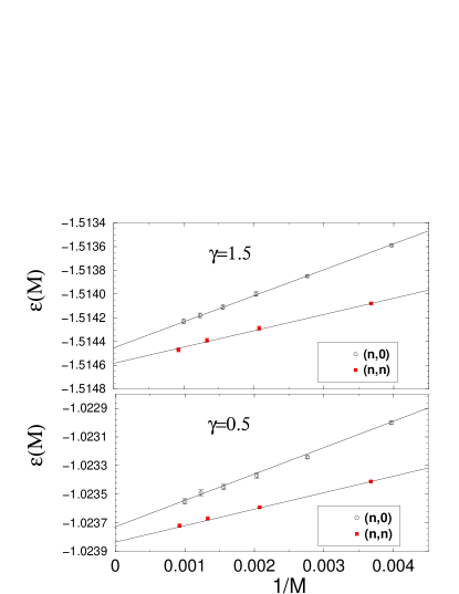
Figure 6: (Color online:) Numerical estimate of $\varepsilon(M)$ as a function of $1/M$ for $(n,0)$ and $(n,n)$ icosadeltahedral lattices with $\gamma=(1.5,0.5)$.

$\gamma$ $a_{1}(\gamma,{\cal Y})$ $(n,n)$ $(n,0)$ $1.875$ $4.45118$ $4.45110(4)$ $4.45095(4)$ $1.75$ $2.47175$ $2.47166(3)$ $2.47150(3)$ $1.625$ $1.82629$ $1.82621(2)$ $1.82603(2)$ $1.5$ $1.51473$ $1.51454(2)$ $1.51445(2)$ $1.375$ $1.33695$ $1.33683(4)$ $1.33667(4)$ $1.25$ $1.22617$ $1.22599(7)$ $1.22589(7)$ $1.125$ $1.15366$ $1.1535(2)$ $1.15340(2)$ $1.0$ $1.10494$ $1.10482(3)$ $1.10464(3)$ $0.875$ $1.07187$ $1.07174(3)$ $1.07160(3)$ $0.75$ $1.04940$ $1.04921(6)$ $1.04910(6)$ $0.625$ $1.03421$ $1.03413(5)$ $1.03398(5)$ $0.5$ $1.02392$ $1.02390(4)$ $1.02372(4)$ $0.375$ $1.01672$ $1.01663(6)$ $1.01656(6)$ $0.25$ $1.01115$ $1.01106(3)$ $1.01103(3)$ $0.125$ $1.00595$ $1.00592(2)$ $1.00589(2)$

Table 2: Numerical values of the coefficient $a_{1}(\gamma,{\cal Y})$ (twelve disclinations on the vertices of an icosahedron) using the $C$-coefficient from Eq.(35). The same coefficients from the $(n,n)$ and $(n,0)$ lattices.

IV.3 The Energy difference of the $(n,m)$ lattices

The $a_{1}$-coefficient computed within our continuum elastic approach above does not depend on the icosadeltahedral class $(n,m)$. Results from the direct minimization of particles do, however, show a weak dependence (in the $4th$ significant digit) on the particular $(n,m)$ configuration, as is apparent from Fig. 2 and Table 2. It should be noted that the discrepancy from the continuum result has a well defined sign, and is therefore reasonably attributed to a term not present in the energy expansion.

V Thomson problem with a continuous distribution of dislocations

When the number of particles is extremely large, the minimum energy configurations can be approximated by a closed analytical form, upon assuming a continuous distribution of defects. Only the sphere will be worked out here, but other curved surfaces can be treated in a very similar fashion.

The formal elimination of the geometric frustration introduced by the Gaussian curvature may be formulated as a concrete set of equations in the case of the sphere. We shall use the identity

$$s({\bf x}) = \frac{\pi}{3\sqrt{g}}\sum_{i=1}^{N}q_{i}\delta({\bf x},{\bf x}_{i})$$

$$= \frac{1}{R^{2}}+\frac{\pi}{3R^{2}}\sum_{l=1}^{\infty}\sum_{m=-l}^{l}Y^{l\ast}_{m}(\theta,\phi)\sum_{i=1}^{N}q_{i}Y^{l\ast}_{m}(\theta_{i},\phi_{i})$$

$$= K({\bf x})+\frac{\pi}{3R^{2}}\sum_{l=1}^{\infty}\sum_{m=-l}^{l}Y^{l\ast}_{m}(\theta,\phi)\sum_{i=1}^{N}q_{i}Y^{l}_{m}(\theta_{i},\phi_{i}),$$

which follows from the topological constraint Eq.(21). Provided a disclination configuration exists such that

$$\sum_{i=1}^{N}q_{i}Y^{l}_{m}(\theta_{i},\phi_{i})=0\ ,$$ (38)

for each $(l\geq 1,m)$, the disclination density completely screens the Gaussian curvature. A configuration of defects satisfying Eq.(38) is an absolute minimum of the elastic energy, a result easily understood by writing the energy in the form

$$E=E_{0}+\frac{\pi^{2}Y}{9}R^{2}\sum_{l=1}^{\infty}\sum_{m=-l}^{l}\frac{\left|\sum_{i=1}^{N}q_{i}Y^{l}_{m}(\theta_{i},\phi_{i})\right|^{2}}{l^{2}(l+1)^{2}}+N\,E_{c}\ ,$$ (39)

where the zero point energy $E_{0}$ in Eq.(16) is kept. A configuration satisfying Eq.(38) will be denoted by ${\cal G}$. For this hypothetical configuration, the $C$-coefficient in Eq.(29) vanishes, although there is now a large contribution (linear in $R$) from the dislocation core energies represented by the last term of Eq.(39).

$\gamma$ $a_{1}(\gamma,{\cal G})$ $\gamma$ $a_{1}(\gamma,{\cal G})$ $\gamma$ $a_{1}(\gamma,{\cal G})$ $\gamma$ $a_{1}(\gamma,{\cal G})$ $1.875$ $4.45227$ $0.875$ $1.07297$ $1.75$ $2.47289$ $0.75$ $1.05044$ $1.625$ $1.82746$ $0.625$ $1.03515$ $1.5$ $1.51592$ $0.5$ $1.02473$ $1.375$ $1.33815$ $0.375$ $1.01737$ $1.25$ $1.22737$ $0.25$ $1.01161$ $1.125$ $1.15485$ $0.125$ $1.00620$ $1$ $1.10610$

Table 3: Value of the $a_{1}$ coefficients for the ${\cal G}$ configuration Eq.(38).

The ${\cal G}$ configuration may be characterized more explicitly. It consists of a density of dislocations that converges to the local Gaussian curvature. It can be shown that upon approximating the dislocations (each regarded as a disclination dipole with spacing $a$) as a continuum distribution, this dislocation density for a sphere becomes

$${\vec{\bf b}}(\theta,\varphi)=\frac{1}{6R}\sum_{k=1}^{6}\cot[\alpha_{k}(\theta,\varphi)]e^{k}_{\varphi}\ .$$ (40)

The summation here runs over the six coordinates of the northern hemisphere of an icosahedron ($(0,0)$ and $(\theta_{\cal Y},\frac{2\pi k}{5})$, where $\theta_{\cal Y}=\arccos(\frac{1}{\sqrt{5}})$ and $\alpha_{k}$ is the angle $\theta$ relative to a coordinate system with the north pole located at $(\theta_{\cal Y},\frac{2\pi k}{5})$ for $k=1,\cdots,5$. This angle is given implicitly by

$$\cos[\alpha_{k}(\theta,\varphi)]=\cos(\theta)\cos(\theta_{\cal Y})-\sin(\theta)\sin(\theta_{\cal Y})\cos(\frac{2\pi}{5}k+\varphi)\ .$$ (41)

The implicit form of Eq.(40) can be further simplified

$${\vec{\bf e}^{k}_{\varphi}} = f^{k}(\theta,\varphi)\left[-\sin(\theta_{\cal Y})\sin(\frac{2\pi}{5}k+\varphi){\vec{\bf e}_{\theta}}\right.$$

$$+ \left.[\{\cos(\theta_{\cal Y})\sin\theta+\sin(\theta_{\cal Y})\}\cos\theta\cos(\varphi+\frac{2\pi}{5}k)]{\vec{\bf e}_{\varphi}}\right]$$

where $f^{k}(\theta,\varphi)=\frac{1}{\sin(\alpha_{k}(\theta,\varphi))}\ .$

Close to one of the 12 disclinations with charge$s=+\frac{2\pi}{6}$ Eq.(40) predicts a singularity in the dislocation density [45]

$$b\approx\frac{s}{2\pi Ra}\ .$$ (43)

For small angles, close to each disclination, there is a short-distance singularity

$$b(\theta)=\frac{\pi}{3R\theta}+\cdots\ ,$$ (44)

in agreement with known results in flat space.

Eq.(40) represents a continuous distribution of dislocations, and neglects both dislocation discreteness and their mutual interactions. It represents six families of dislocations with azimuthal Burgers’ vectors associated with antipodal pairs of the 12 original disclinations in the icosahedron. When discreteness and interactions are taken in account, we expect these dislocations to condense into grain boundary arms, containing with quantized Burgers’ vectors and variable spacing in the radial direction [21, 44, 57]. The total number of discrete arms remains, therefore, the variable that needs to be determined for a discrete solution of the Thomson problem.

V.1 The intermediate regime

Within the continuum elastic approach, the dominant configurations for a small number of particles are 12 defects with an icosahedral symmetry [21]. We have just seen, however, that adding a continuous distribution of dislocations, as might be appropriate when the particle number is large, can more efficiently screen the Gaussian curvature on a sphere. The natural problem then becomes to determine the precise structure of the defect arrays for intermediate numbers of particles when the discreteness of interacting dislocations is taken into account.

Figure 7: Results of a minimization of 500 particles interacting with a Coulomb potential, showing the appearance of scars.

We note first that the particular arrangement of defects dominating in this regime will not be fully universal. The particular array structure favored can vary from system to system with fixed particle number, depending, e.g., on details such as the dislocation core energy. This result may be traced back to the $M$-expansion of Eq.(34), in which the sub-leading terms which depend on non-universal properties influence the dominant terms for finite values of $M$. Some typical defect configurations obtained by direct minimization of particles on the sphere are shown in Fig. 7 and show incipient scars, already at number of particles of 500 (in [21, 53] the minimum number of particles where scars are systematically found is predicted around 400). By using the geometrical model described in this paper, where the energy is parameterized just by a Young’s modulus and a dislocation core energy [21, 22] one can simulate larger particle numbers and one obtains results as in Fig. 8. Note the occurrence of low energy configurations with scars ($m=2$) in one instance and pentagonal buttons ($m=5$) in another. The dislocation spacing decreases the further a dislocation is from the central disclination.

Figure 8: Ground state configurations for $M\approx 2000$ particles obtained from the continuum elastic formalism. In the top figure one finds scars ($m=2$) and in the bottom pentagonal buttons ($m=5$) forming a rhombic tricontahedron.

An overview of previous results involving grain boundary scars is presented in Fig. 9. If a disclination is placed on a perfect crystal, no additional defects will appear if the disclination is located on the tip of a cone with total Gaussian curvature equal to the disclination charge. If a disclination is forced into a flat monolayer, then $m$ low angle grain boundaries, with constant spacing between dislocations as shown in Fig. 9 and grains going all the way to the boundary, will be favored (see [44] for a detailed discussion). In the intermediate situation where a finite Gaussian curvature is spread over a finite area, as in the case of a spherical cap, a disclination arises at the center of the cap, and finite length grain boundaries stretched out over an area of $\frac{\pi}{3}R^{2}$ with variable spacing dominate, again as illustrated in Fig. 9. Since several non-universal features, related to the size of the core energies, commensurability properties and so on, will have an important effect in this regime of $M$, the previous argument should describe the general trends and will be realized in an approximate form only.

Figure 9: Schematic illustrating the genesis of grain boundary scars. A disclination is first constructed from a perfect lattice. If this disclination is placed on a tip of a cone, with a delta function of Gaussian curvature balancing the defect charge, then no additional defects form. If the crystal is forced into a monolayer, grain boundaries radiating out of the disclination radiate all the way to the boundary. In the intermediate regime of constant non-zero Gaussian curvature, $m$ grain boundaries of finite length and variable spacing of dislocations form.

Additional results may be obtained for the number of arms within the grain boundary, the actual variable spacing between dislocations within the grain and the length of the grains as a function of the number of particles. The detailed study of these questions will be reported elsewhere.

When grain boundary scars appear, we can estimate the number of excess dislocations which decorate each of the 12 curvature-induced disclinations on the sphere using ideas from Ref.[21]. This estimate is in reasonable agreement with experiments probing equilibrated assemblies of polystyrene beads on water droplets [22]. Consider the region surrounding one of the 12 excess disclinations, with charge $s=2\pi/6$, centered on the north pole. As discussed in Ref.[21], we expect the stresses and strains at a fixed geodesic distance $r$ from the pole on a sphere of radius $R$ to be controlled by an effective disclination charge

$$s_{eff}(r) = s-\int^{2\pi}_{0}{\rm d}\phi\int^{r}_{0}{\rm d}r^{\prime}\sqrt{g(r)}\,K$$ (45)

$$= \pi/3-4\pi{\rm sin}^{2}(\frac{r}{2R})\,.$$

Here the Gaussian curvature is $K=1/R^{2}$ and the metric tensor associated with spherical polar coordinates $(r,\phi)$, with distance element $ds^{2}=d^{2}r+R^{2}\sin^{2}(r/R)d^{2}\phi$, gives $\sqrt{g(r)}=R\sin(r/R)$. Suppose m grain boundaries radiate from the disclination at the north pole. Then, in an approximation which neglects interactions between the individual arms, the spacing between the dislocations in these grains is [21]

$$l(r)=\frac{am}{s_{eff}(r)}\ ,$$ (46)

which implies an effective dislocation density

$$n_{d}(r) = \frac{1}{l(r)}$$ (47)

$$= \frac{1}{ma}\bigg{[}\frac{\pi}{3}-4\pi\sin^{2}(r/2R)\bigg{]}$$

$$= \frac{2\pi}{ma}\bigg{[}\cos\frac{r}{R}-5/6\bigg{]}\ .$$

This density vanishes when $r\rightarrow r_{c}$, where

$$r_{c}=R\cos^{-1}5/6\approx R(33.56^{\circ})\ ,$$ (48)

which is the distance at which the $m$ grain boundaries terminate. The total number of dislocations residing within this radius is thus

$$N_{d} = m\int^{r_{c}}_{0}n_{d}(r)dr$$ (49)

$$= \frac{r_{c}}{a}\frac{\pi}{3}-\frac{4\pi}{a}\int^{r_{c}}_{0}\sin^{2}(r/2R)dr$$

$$= \frac{\pi}{3}\bigg{[}\sqrt{11}-5\cos^{-1}(5/6)\bigg{]}(R/a)$$

$$\approx 0.408(R/a)\ .$$

As discussed in Ref.[37], it is also of interest to consider $2\pi$ disclination defects (appropriate to crystals of tilted molecules [59]) on the sphere. The icosahedral configuration of 12 $s=2\pi/6$ disclinations is now replaced by just two $s=2\pi$ disclinations at the north and south poles. Using the approximation discussed above, it is straightforward to show that the density of dislocations in each of $m$ (noninteracting) grain boundary arms now reads

$$n_{d}(r)=\frac{2\pi}{ma}\cos\big{(}\frac{r}{R}\big{)}\ .$$ (50)

This density vanishes at $r_{c}=\frac{\pi}{2}R$, corresponding to a hemisphere of area on the sphere for each cluster of arms.

It is of considerable interest to repeat the above calculation for a square lattice, as found for example in the protein surface layers (s-layers) of some bacteria [47, 48]. In this case the basic disclination has $s=2\pi/4$. The effective dislocation density becomes

$$n_{d}(r) = \frac{1}{l(r)}$$ (51)

$$= \frac{1}{ma}\bigg{[}\frac{\pi}{2}-4\pi\sin^{2}(r/2R)\bigg{]}$$

$$= \frac{2\pi}{ma}\bigg{[}\cos\frac{r}{R}-3/4\bigg{]}\ .$$

This density vanishes when $r\rightarrow r_{c}$, where

$$r_{c}=R\cos^{-1}3/4\approx R(41.4^{\circ})\ ,$$ (52)

which is the distance at which the $m$ grain boundaries terminate. The longer angular length of square lattice scars reflects the larger initial disclination charge ($90^{\circ}$) that must be screened. The total number of dislocations residing within this radius is thus

$$N_{d} = m\int^{r_{c}}_{0}n_{d}(r)dr$$ (53)

$$= \frac{r_{c}}{a}\frac{\pi}{2}-\frac{4\pi}{a}\int^{r_{c}}_{0}\sin^{2}(r/2R)dr$$

$$= \frac{\pi}{2}\bigg{[}\sqrt{7}-3\cos^{-1}(3/4)\bigg{]}(R/a)$$

$$\approx 0.75(R/a)\ .$$

Thus the angular length of scars and the total number of excess dislocations is a measure of the underlying topology of the lattice tiling the sphere.

VI Conclusions

VI.1 Summary of Results

In this section we summarize the most relevant results obtained from the analysis presented earlier.

In Sect. II we treated several properties of planar and spherical crystals which were subsequently used to test our continuum elastic formalism. We computed the energy Eq.(II.1) and elastic tensor Eq.(9) for triangular lattices in flat space for a general long range power law potential of the type Eq.(2). The continuum elastic formalism, where defects such as disclinations and disclination dipoles $\equiv$ dislocations are the relevant degrees of freedom and six-coordinated particles are treated as a continuous elastic background, was discussed in Sect. III. It was shown that the total energy is expressible as an expansion in powers in the total number of particles [Eq.(29)]:

$$2E = \left(\frac{M^{2}}{2^{\gamma-1}(2-\gamma)}-a_{1}(\gamma|\{q_{i}\}_{i=1,\cdot,N})M^{1+\gamma/2}\right.$$

$$- \left.a_{2}(\gamma|\{q_{i}\}_{i=1,\cdot,N})M^{\gamma/2}\right)\frac{e^{2}}{R^{\gamma}}$$

where each coefficient has a clear geometric interpretation in terms of continuum results.

Our approach was illustrated for the generalized Thomson problem in Sect IV. Using the elastic constants computed in flat space, the continuum elastic theory gives concrete energy predictions, with no fitting parameters, as a series expansion in the total number of particles $M$, which can be compared with the energies obtained numerically for spherical crystals. We find agreement to 5 significant figures for $(n,n)$ icosadeltahedral lattices and to 4 significant figures for $(n,0)$ lattices, as presented in Table 2. Only a small discrepancy, of order the difference between $(n,0)$ and $(n,n)$ tessellations, separates the continuum results from results for actual spherical crystals.

The limit of a very large number of particles $M$ was dealt with in Sect V. A “Debye-Huckel” type formulation where dislocations are treated in a smeared continuum density of Burgers’ vectors was proposed. In Ref.[57] an explicit solution for the actual defect distribution without assuming a continuum of dislocations was proposed and it was shown that certain dislocation grain boundaries have a $C$-coefficient that vanishes in the limit of a very large number of particles ($R/a\rightarrow\infty)$. This solution is a discrete version of the continuum solution presented in this paper, and incorporates the discreteness of the dislocation positions and charges and their mutual interactions. We should mention that an alternative scenario for the Thomson problem has been proposed [58], where at some finite value of number of particles an instability to a “spontaneously magnetized” state is predicted. Based on the results presented in this paper and in Ref.[57, 36] we conclude that such instability does not appear for the generalized Thomson problem. It is possible that an instability of the type predicted in [58] may appear for charges on spheres under other type of constraints.

The intermediate regime was discussed in the last section and it was shown that the underlying universality of the result competes with several non-universal features of the problem.

VI.2 Outlook

The main goal of this paper was to introduce a continuum elastic approach to address the problem of two-dimensional crystals in frozen topographies. The formalism has been explicitly applied to the sphere, but it appears general enough to be applicable to a variety of other geometries. The case of crystalline order on a torus is currently under exploration.

We hope this presentation will inspire further work on the problem of crystals on curved topographies. The long range pair interactions on a sphere studied here certainly do not exhaust the possible problems.

ACKNOWLEDGMENTS

Our interest in this problem is the result of numerous discussions with Alar Toomre. MJB would like to thank Cris Cecka and Alan Middleton for discussions and for extensive work on Java simulations of the generalized Thomson problem. The work of MJB was supported by the NSF through Grant No. DMR-0219292 (ITR). The work of DRN was supported by the NSF through Grant No. DMR-0231631 and through the Harvard Material Research Science and Engineering Laboratory via Grant No. DMR-0213805. The work of AT was supported by the NSF through Grant No. DMR-0426597 and partially supported by the US Department of Energy (DOE) under contract No. W-7405-ENG-82 and Iowa State Start-up funds.

Appendix A The evaluation of Potentials

The details of the computation of the energy and the elastic tensor, Eqs.(II.1) and Eq.(9) are described in detail. The approach followed is a generalization of the one used by Bonsall and Maradudin [60]. See also ref [61].

A.1 Computation of the energy

The energy for a system of $M$ particles located at positions ${\vec{R}}({\bf l})$ of a 2d Bravais lattice, defined by vectors ${\bf a}_{i}$ and ${\bf e}_{i}$ in direct and reciprocal space

$${\vec{R}}({\bf l}) = l_{1}{\bf a}_{1}+l_{2}{\bf a}_{2}$$ (55)

$${\vec{G}}({\bf h}) = h_{1}{\bf e}_{1}+h_{2}{\bf e}_{2}$$ (56)

is given by Eq.(5)

$$E_{0} = \frac{e^{2}}{2}\sum_{{\bf l}\neq{\bf l}^{\prime}}^{M}\frac{1}{|{\vec{R}}({\bf l})-{\vec{R}}({\bf l}^{\prime})|^{\gamma}}$$ (57)

$$= M\frac{e^{2}}{2}\lim_{\vec{x}\rightarrow 0}\sum_{l\neq 0}\frac{1}{|\vec{x}-{\vec{R}}({\bf l})|^{\gamma}}\equiv\frac{M}{2}E(\gamma)\ .$$

To efficiently perform the sum (a generalization of the Ewald method), we separate short and long distances contributions, since they give rise to different singular behavior. This may be achieved by the identity Eq.(76)

$$\frac{1}{|{\vec{x}}-{\vec{R}}({\bf l})|^{\gamma}} = \frac{1}{\Gamma(\frac{\gamma}{2})}\left\{\int^{\infty}_{\sigma}dtt^{-1+\gamma/2}e^{-t|{\vec{x}}-{\vec{R}}({\bf l})|^{2}}\right.$$

$$+ \left.\int^{\sigma}_{0}dtt^{-1+\gamma/2}e^{-t|{\vec{x}}-{\vec{R}}({\bf l})|^{2}}\right\}$$

$$= \frac{\sigma^{\gamma/2}}{\Gamma({\frac{\gamma}{2}})}\varphi_{\gamma/2-1}(\sigma|{\vec{x}}-{\vec{R}}({\bf l})|^{2})$$

$$+ \frac{\sigma^{\gamma/2}}{\Gamma({\frac{\gamma}{2}})}\int^{1}_{0}dtt^{-1+\frac{\gamma}{2}}e^{-t\sigma|{\vec{x}}-{\vec{R}}({\bf l})|^{2}}$$

The definition of the Misra functions $\varphi_{n}$ is given below in Eq.(77).

Using the Poisson summation formula Eq.(• ‣ B.1), the last term in Eq.(A.1) can also be expressed in terms of Misra functions,

$$\sum_{l}\int^{1}_{0}dtt^{-1+\gamma/2}e^{-t\sigma|{\vec{x}}-{\vec{R}}({\bf l})|^{2}} =$$ (59)

$$\frac{\pi}{A_{C}\sigma}\sum_{\vec{G}}e^{i{\vec{G}}\cdot{\vec{x}}}\int^{\infty}_{1}dtt^{-\frac{\gamma}{2}}e^{-t\frac{|{\vec{G}}|^{2}}{4\sigma}} =$$

$$\frac{\pi}{A_{C}\sigma}\sum_{\vec{G}}e^{i{\vec{G}}\cdot{\vec{x}}}\varphi_{-\gamma/2}(\frac{|{\vec{G}}|^{2}}{4\sigma})$$

where ${\vec{G}}$ are the vectors in reciprocal space of the Bravais lattice, and $A_{C}$ is the area of the unit cell.

Upon combining Eq.(A.1) and Eq.(59), the energy Eq.(57) becomes

$$E(\gamma) = \frac{\sigma^{\gamma/2}e^{2}}{\Gamma(\frac{\gamma}{2})}\sum_{l\neq 0}\varphi_{\gamma/2-1}(\sigma|{\vec{x}}-{\vec{R}}({\bf l})|^{2})-\frac{2\sigma^{\gamma/2}}{\gamma\Gamma(\gamma/2)}e^{2}$$ (60)

$$+ \frac{\pi e^{2}\sigma^{\gamma/2-1}}{A_{C}\Gamma(\gamma/2)}\sum_{\vec{G}}e^{i{\vec{G}}\cdot{\vec{x}}}\varphi_{-\gamma/2}(\frac{|{\vec{G}}|^{2}}{4\sigma})$$

Although the limit ${\vec{x}}\rightarrow 0$ is in general convergent, the term ${\vec{G}}=0$ requires special attention. This term has to be treated separately by considering $|\vec{G}|$ small but non-vanishing,

$$\frac{\pi e^{2}\sigma^{\gamma/2-1}}{\Gamma(\gamma/2)}e^{i{\vec{G}}{\bf x}}\varphi_{-\gamma/2}(\frac{|{\vec{G}}|^{2}}{4\sigma}) = \frac{\pi 2^{2-\gamma}\Gamma(1-\gamma/2)}{|{\vec{G}}|^{2-\gamma}\Gamma(\gamma/2)}e^{2}$$ (61)

$$- \frac{\pi\sigma^{\gamma/2-1}}{A_{C}\Gamma(\gamma/2)(1-\gamma/2)}e^{2}$$

$$+ {\cal O}(|{\vec{G}}|).$$

Thus, the singularity as ${\vec{G}}\rightarrow 0$, associated with the large distance behavior, has been explicitly isolated.

The results derived so far are completely general, valid for any Bravais lattice. Since only the triangular lattice is relevant to this paper, complete results for other Bravais lattices will be published elsewhere. The two vectors ${\bf a}_{1},{\bf a}_{2}$ defining the triangular lattice in direct space, and the two vectors ${\bf e}_{1},{\bf e}_{2}$ in reciprocal space are taken as

$${\bf a}_{1}=(a,0) {\bf e}_{1}=\frac{2\pi}{a}(1,-\frac{\sqrt{3}}{3})$$ ,

$${\bf a}_{2}=(\frac{a}{2},\frac{\sqrt{3}a}{2}) {\bf e}_{2}=\frac{2\pi}{a}(0,2\frac{\sqrt{3}}{3})\ ,$$ , (62)

where $a$ is the lattice constant. Further simplification is achieved by choosing $\sigma$ as $\sigma=\frac{\pi}{A_{C}}$ (where $A_{C}=\frac{\sqrt{3}}{2}a^{2}$), so that the argument in the Misra functions has a similar form for the sums in both direct and reciprocal space. Thus,

$$\sigma{\vec{R}}^{2}({\bf l}) = \frac{\pi}{A_{0}}(l_{1}^{2}{\bf a}_{1}^{2}+2l_{1}l_{2}{\bf a}_{1}{\bf a}_{2}+l_{2}^{2}{\bf a}_{2}^{2})$$ (63)

$$\frac{{\bf G}^{2}(h)}{4\sigma} = \frac{1}{4\sigma}(h_{1}^{2}{\bf e}_{1}^{2}+2h_{1}h_{2}{\bf e}_{1}{\bf e}_{2}+h_{2}^{2}{\bf e}_{2}^{2})$$

$$= \frac{\pi}{A_{0}}(h_{1}^{2}{\bf a}_{1}^{2}-2h_{1}h_{2}{\bf a}_{1}{\bf a}_{2}+h_{2}^{2}{\bf a}_{2}^{2})\ .$$

Our final form for the energy is then

$$E(\gamma) = -\frac{e^{2}}{\Gamma(\gamma/2)}\left\{(\frac{\pi}{A_{C}})^{\gamma/2}\{\frac{4}{\gamma(2-\gamma)}\right.$$ (65)

$$- \left.\sum_{l\neq 0}\varphi_{-\gamma/2}(\frac{\pi}{A_{C}}{\vec{R}}^{2}({\bf l}))-\sum_{l\neq 0}\varphi_{\gamma/2-1}(\frac{\pi}{A_{C}}{\vec{R}}^{2}({\bf l}))\}\right\}$$

$$+ \lim_{|{\vec{G}}|\rightarrow 0}\frac{\pi 2^{2-\gamma}\Gamma(1-\gamma/2)}{A_{C}|{\vec{G}}|^{2-\gamma}\Gamma(\gamma/2)}e^{2}.$$

The summation over the Misra functions is exponentially convergent; just a few terms give a very accurate result.

A.2 Computation of the elastic tensor

The response function is defined in Eq.(8). Using some simple algebra, the explicit form for this tensor response function $\Pi$ follows

$$\Pi_{\alpha,\beta}({\bf l},{\bf l}^{\prime})=\left\{\begin{array}[]{l c}-\gamma(\gamma+2)\frac{({\vec{R}}({\bf l})-{\vec{R}}({\bf l}^{\prime}))_{\alpha}({\vec{R}}({\bf l})-{\vec{R}}({\bf l}^{\prime}))_{\beta}}{|({\vec{R}}({\bf l})-{\vec{R}}({\bf l}^{\prime})|^{\gamma+4}}+&\\ +\gamma\frac{\delta_{\alpha\beta}}{|({\vec{R}}({\bf l})-{\vec{R}}({\bf l}^{\prime})|^{\gamma+2}}&{\bf l\neq l^{\prime}}\\ -\sum_{l\neq l^{\prime}}\Pi_{\alpha\beta}({\bf l},{\bf l}^{\prime})&{\bf l=l^{\prime}}\end{array}\right.$$ (66)

The property ${\vec{R}}({\bf l})-{\vec{R}}({\bf l}^{\prime})={\vec{R}}({\bf l}-{\bf l}^{\prime})-{\vec{R}}(0)$ implies translational invariance $\Pi({\bf l},{\bf l}^{\prime})=\Pi({\bf l}-{\bf l}^{\prime},0)$. The response function is better studied in Fourier space. The Fourier transformed elastic tensor can be computed from the identity

$$\Pi_{\alpha\beta}(\vec{p})=-(S_{\alpha\beta}(\vec{p})-S_{\alpha\beta}(\vec{0}))\ ,$$ (67)

with $S_{\alpha\beta}$ defined as

$$S_{\alpha\beta}(\vec{p}) = \lim_{{\vec{x}}\rightarrow 0}\frac{\partial^{2}}{\partial_{\alpha}\partial_{\beta}}\left(e^{-i{\vec{p}}\cdot{\vec{x}}}\sum_{l\neq 0}e^{i{\vec{p}}({\vec{x}-\vec{R}}({\bf l}))}\frac{1}{|{\vec{x}}-{\vec{R}}({\bf l})|^{\gamma}}\right)$$ (68)

$$= \lim_{\vec{x}\rightarrow 0}\frac{\partial^{2}}{\partial_{\alpha}\partial_{\beta}}{\cal F}({\vec{x}},{\vec{p}})$$

$${\cal F}({\vec{x}},{\vec{p}})\equiv\sum_{l}\frac{e^{i{\vec{p}}\cdot({\vec{x}}-{\vec{R}}({\bf l}))}}{|{\vec{x}}-{\vec{R}}({\bf l})|^{\gamma}}\ ,$$

The function ${\cal F}$ can be computed by further using Eq.(A.1), Eq.(59) and Eq.(• ‣ B.1), with essentially the same steps as in previous computations, leading to the expression

$${\cal F}({\vec{x}},{\vec{p}}) = \frac{\sigma^{\gamma/2}}{\Gamma(\gamma/2)}\sum_{l\neq 0}e^{-i{\vec{p}}{\vec{R}}({\bf l})}\varphi_{\gamma/2-1}(\sigma|{\vec{x}}-{\vec{R}}({\bf l})|^{2})$$ (69)

$$- \frac{\sigma^{\gamma/2}}{\Gamma(\gamma/2)}\int^{1}_{0}dtt^{-1+\gamma/2}e^{-t|{\vec{x}}|^{2}\sigma}$$

$$+ \frac{\pi\sigma^{\gamma/2-1}}{A_{C}\Gamma(\gamma/2)}\sum_{{\vec{G}}\neq 0}e^{i({\vec{p}}+{\vec{G}})\cdot{\vec{x}}}\varphi_{-\gamma/2}(\frac{|{\vec{p}}+{\vec{G}}|^{2}}{4\sigma})$$

$$+ \frac{\pi\sigma^{\gamma/2-1}}{A_{C}\Gamma(\gamma/2)}\varphi_{-\gamma/2}(\frac{|{\vec{p}}+{\vec{G}}|^{2}}{4\sigma})\ .$$

Upon inserting the derivatives of the Misra functions obtained from Eq.(78), Eq.(• ‣ B.1) and using Eq.(68), we have

$$S_{\alpha\beta}({\vec{p}}) = -\frac{\pi\sigma^{\gamma/2-1}}{A_{C}\Gamma(\gamma/2)}\sum_{\vec{G}}(\vec{p}+\vec{G})_{\alpha}(\vec{p}+\vec{G})_{\beta}\;\varphi_{-\gamma/2}(\frac{|{\vec{p}}+{\vec{G}}|^{2}}{4\sigma})$$ (70)

$$- \frac{2\sigma^{\gamma/2+1}}{\Gamma(\gamma/2)}\sum_{l\neq 0}e^{-i{\vec{p}}\cdot{\vec{R}}({\bf l})}\;\varphi_{\gamma/2}(\sigma|{\vec{R}}({\bf l})|^{2})$$

$$- \frac{4\sigma^{\gamma/2+2}}{\Gamma(\gamma/2)}\sum_{l\neq 0}{\vec{R}}({\bf l})_{\alpha}{\vec{R}}({\bf l})_{\beta}\;\varphi_{1+\gamma/2}(\sigma|{\vec{R}}({\bf l})|^{2})\$$

$$+ \frac{4}{2+\alpha}\frac{\sigma^{\gamma/2+1}}{\Gamma(\gamma/2)}.$$

The full expression for the response function is then

$$\Pi_{\alpha\beta}({\vec{p}}) = \frac{\pi\sigma^{\gamma/2-1}}{A_{C}\Gamma(\gamma/2)}\sum_{\bf G}(\vec{p}+\vec{G})_{\alpha}(\vec{p}+\vec{G})_{\beta}\varphi_{-\gamma/2}(\frac{|{\vec{p}}+{\vec{G}}|^{2}}{4\sigma})-\frac{\pi\sigma^{\gamma/2-1}}{A_{C}\Gamma(\gamma/2)}\sum_{\vec{G}}\vec{G}_{\alpha}\vec{G}_{\beta}\;\varphi_{-\gamma/2}(\frac{|{\vec{G}}|^{2}}{4\sigma})$$ (71)

$$+ \frac{2\sigma^{\gamma/2+1}}{\Gamma(\gamma/2)}\sum_{l\neq 0}(e^{-i{\vec{p}}\cdot{\vec{R}}({\bf l})}-1)\;\varphi_{\gamma/2}(\sigma|{\vec{R}}({\bf l})|^{2})-\frac{4\sigma^{\gamma/2+2}}{\Gamma(\gamma/2)}\sum_{l\neq 0}(e^{-i{\vec{p}}\cdot{\vec{R}}({\bf l})}-1){\vec{R}}({\bf l})_{\alpha}{\vec{R}}({\bf l})_{\beta}\varphi_{1+\gamma/2}(\sigma|{\vec{R}}({\bf l})|^{2}\ .$$

As in the computation of the energy, it is convenient to isolate the ${\vec{G}}\rightarrow 0$ contribution since it usually gives raise to non-analyticities. A Taylor expansion for the ${\bf G}\rightarrow 0$ contribution leads to a final expression

$$\Pi_{\alpha\beta}({\vec{p}}) = \frac{2^{2-\gamma}\pi\Gamma(1-\gamma/2)}{A_{C}\Gamma(\gamma/2)}\frac{\vec{p}_{\alpha}\vec{p}_{\beta}}{|{\vec{p}}|^{2-\gamma}}+\frac{2^{2-\gamma}\pi\Gamma(1-\gamma/2)}{A_{C}\Gamma(\gamma/2)}\frac{\vec{p}_{\alpha}\vec{p}_{\beta}}{|{\vec{p}}|^{2-\gamma}}\left(\frac{1}{\Gamma(1-\gamma/2)}(\frac{{\vec{p}}^{2}}{4\sigma})^{1-\gamma/2}\varphi_{-\gamma/2}(\frac{{\vec{p}}^{2}}{4\sigma})-1\right)$$

$$+ \frac{\pi\sigma^{\gamma/2-1}}{A_{C}\Gamma(\gamma/2)}\sum_{\vec{G}}(\vec{p}+\vec{G})_{\alpha}(\vec{p}+\vec{G})_{\beta}\varphi_{-\gamma/2}(\frac{|{\vec{p}}+{\vec{G}}|^{2}}{4\sigma})-\frac{\pi\sigma^{\gamma/2-1}}{A_{C}\Gamma(\gamma/2)}\sum_{\vec{G}}\vec{G}_{\alpha}\vec{G}_{\beta}\;\varphi_{-\gamma/2}(\frac{|{\vec{G}}|^{2}}{4\sigma})]$$

$$- \frac{2\sigma^{\gamma/2+1}}{\Gamma(\gamma/2)}\sum_{{\bf l}\neq 0}[1-\cos({\vec{p}}\cdot{\vec{R}}({\bf l}))]\;\varphi_{\gamma/2}(\sigma|{\vec{R}}({\bf l})|^{2})+\frac{4\sigma^{\gamma/2+2}}{\Gamma(\gamma/2)}\sum_{{\bf l}\neq 0}[1-\cos({\vec{p}}\cdot{\vec{R}}({\bf l}))]{\vec{R}}({\bf l})_{\alpha}{\vec{R}}({\bf l})_{\beta}\varphi_{1+\gamma/2}(\sigma|{\vec{R}}({\bf l})|^{2})\ .$$

Since all the terms in the previous expression but the first one are analytical functions of the momentum, the response function at large distances goes like

$$\Pi_{\alpha\beta}({\vec{p}}) = \frac{2^{2-\gamma}\pi\Gamma(1-\gamma/2)}{A_{C}\Gamma(\gamma/2)}\frac{\vec{p}_{\alpha}\vec{p}_{\beta}}{|{\vec{p}}|^{2-\gamma}}$$

$$+ A_{\alpha\beta\mu\nu}\vec{p}^{\mu}\vec{p}^{\nu}+B_{\alpha\beta\mu\nu\rho\zeta}{\vec{p}}^{\mu}\vec{p}^{\nu}\vec{p}^{\rho}\vec{p}^{\zeta}+{\cal O}(\vec{p}^{6})\$$

The results derived are valid for any Bravais lattice. Again, only the triangular lattice is of interest in this paper. The tensor $A_{\alpha\beta\mu\nu}$ for the triangular lattice is

$$A_{\alpha\beta\mu\nu} = -\frac{\delta_{\mu\nu}}{4\Gamma(\gamma/2)}(\frac{\pi}{A_{c}})^{\gamma/2-1}\sum_{{\bf l}\neq 0}G_{\alpha}({\bf l})G_{\beta}({\bf l})\varphi_{1-\gamma/2}(\frac{\pi}{A_{C}}{\vec{R}}^{2}({\bf l}))$$

$$- \frac{\delta_{\alpha\mu}\delta_{\beta\nu}+\delta_{\alpha\nu}\delta_{\beta\mu}}{2\Gamma(\gamma/2)}(\frac{\pi}{A_{C}})^{\gamma/2}\left[\frac{2}{2-\gamma}-\sum_{l\neq 0}\varphi_{-\gamma/2}(\frac{\pi}{A_{C}}{\vec{R}}^{2}({\bf l}))\right]$$

$$- \frac{1}{4^{\ddagger}\Gamma(\gamma/2)}(\frac{\pi}{A_{C}})^{\gamma/2-1}\sum_{{\bf l}\neq 0}\left[(G_{\alpha}({\bf l})G_{\mu}({\bf l})\delta_{\beta\nu}+G_{\beta}({\bf l})G_{\nu}({\bf l})\delta_{\alpha\mu}+G_{\alpha}({\bf l})G_{\nu}({\bf l})\delta_{\beta\mu}+G_{\beta}({\bf l})G_{\mu}({\bf l})\delta_{\alpha\nu})\;\varphi_{1-\gamma/2}(\frac{\pi}{A_{C}}{\vec{R}}^{2}({\bf l}))\right]$$

$$+ \frac{1}{8\Gamma(\gamma/2)}(\frac{\pi}{A_{C}})^{\gamma/2-2}\sum_{{\bf l}\neq 0}G_{\alpha}({\bf l})G_{\beta}({\bf l})G_{\mu}({\bf l})G_{\nu}({\bf l})\;\varphi_{2-\gamma/2}(\frac{\pi}{A_{C}}{\vec{R}}^{2}({\bf l}))$$

$$+ \frac{2}{\Gamma(\gamma/2)}(\frac{\pi}{A_{C}})^{\gamma/2+2}\sum_{{\bf l}\neq 0}R_{\alpha}({\bf l})R_{\beta}({\bf l})R_{\mu}({\bf l})R_{\nu}({\bf l})\;\varphi_{1+\gamma/2}(\frac{\pi}{A_{C}}{\vec{R}}^{2}({\bf l}))$$

$$- \frac{\delta_{\mu\nu}}{\Gamma(\gamma/2)}(\frac{\pi}{A_{C}})^{\gamma/2+1}\sum_{{\bf l}\neq 0}R_{\alpha}({\bf l})R_{\beta}({\bf l})\;\varphi_{\gamma/2}(\frac{\pi}{A_{C}}{\vec{R}}^{2}({\bf l}))\$$

The form of the elastic tensor can be parameterized by two coefficients $\theta(\gamma)$ and $\eta(\gamma)$

$$A_{\alpha\beta\mu\nu}=\frac{\eta(\gamma)}{A^{\gamma/2}}[\delta_{\mu\nu}\delta_{\alpha\beta}+\rho(\gamma)(\delta_{\mu\alpha}\delta_{\nu\beta}+\delta_{\mu\beta}\delta_{\nu\alpha}]\ ,$$ (75)

a result that can just follows from the symmetry properties of the triangular lattice [62]

Appendix B Mathematical identities used

In this section useful mathematical identities are listed without further remarks to make the paper as self-contained as possible and for the purpose of fixing the notation.

B.1 Identities present in Ewald Sums

• The Gamma identity

  $$\frac{1}{|{\vec{x}}|^{\gamma}}=\frac{1}{\Gamma(\frac{\gamma}{2})}\int^{\infty}_{0}dtt^{-1+\frac{\gamma}{2}}e^{-t|{\vec{x}}|^{2}}$$ (76)

• Misra function definition

  $$\varphi_{n}(z)=\int^{\infty}_{1}dt\,t^{n}e^{-zt}$$ (77)

• Misra function derivatives

  $$\nabla_{\vec{x}}\varphi_{n}(a|{\vec{x}}-{\vec{m}}|^{2})=-2a({\vec{x}}-{\vec{m}})\varphi_{1+n}(a|{\vec{x}}-{\vec{m}}|^{2})$$ (78)

  $$\frac{\partial^{2}}{\partial_{\alpha}\partial_{\beta}}\varphi_{n}(a|{\vec{x}}-{\vec{m}}|^{2})=-2a\delta_{\alpha\beta}\varphi_{1+n}(a|{\vec{x}}-{\vec{m}}|^{2})$$

  $$+4a^{2}(\vec{x}-\vec{m})_{\alpha}(\vec{x}-\vec{m})_{\beta}\varphi_{n+2}(a|{\vec{x}}-{\vec{m}}|^{2})$$ (79)

• Poisson summation formula for Gaussian integrals

  $$\sum_{l}e^{i{\vec{q}}\cdot({\vec{x}}-{\vec{R}}(n))}e^{-t\sigma|{\vec{x}}-{\vec{R}}({\bf l})|^{2}} =$$

  $$\frac{\pi}{A_{C}t\sigma}\sum_{\vec{G}}e^{i({\vec{G}}+{\vec{q}})\cdot{\vec{x}}}e^{-\frac{|{\vec{q}}+{\vec{G}}|^{2}}{4t\sigma}}$$ (80)

References

- [1] J. J. Thomson, Philos. Mag. 7, 237 (1904).
- [2] E.B. Saff and A.B.J. Kuijlaars, Math. Intelligencer 19, 5 (1997).
- [3] D.P. Hardin and E.B. Saff, Notices of the Amer. Math. Soc. 51, 1186 (2005).
- [4] D.P. Hardin and E.B. Saff, Adv. in Mathematics 193, 174 (2005) [http://arxiv.org/abs/math-ph/0311024].
- [5] U. Albrecht and P. Leiderer, J. Low Temp. Phys. 86, 131 (1992).
- [6] P. Leiderer, Z. Phys. B 98, 303 (1993).
- [7] C.C. Grimes and G. Adams, Phys. Rev. Lett. 42, 795 (1979).
- [8] D.C. Glattli, E.Y. Andrei, and F.I.B. Williams, Phys. Rev. Lett. 60, 420 (1998).
- [9] P. Lenz and D.R. Nelson, Phys. Rev. Lett. 87, 125703 (2001) [http://arxiv.org/abs/cond-mat/0104062]; Phys. Rev. E 67, 031502 (2003) [http://arxiv.org/abs/cond-mat/0211140].
- [10] E.J. Davis, Aerosol Sci. Techn. 26, 212 (1997).
- [11] D.L.D. Caspar and A. Klug, Cold Spring Harb Symp. Quant Biol. 27, 1 (1962).
- [12] C.J. Marzec and L. A. Day, Biophys. J. 255, 1 (1993).
- [13] X. Yan, N.H. Olson, J.L. Van Etten, M. Bergoin, M.G. Rossmann, and T.S. Baker, Nature Structural Biol. 7, 101 (2000).
- [14] T.S. Baker, N.H. Olson and S.D. Fuller, Microbiol. Mol. Biol. Rev. 63, 862 (1999).
- [15] R. Zandi, D. Reguera, R.F. Bruinsma, W.M. Gelbart, and J. Rudnick, Proc. Natl. Acad. Sci. USA 101, 15556 (2004).
- [16] J. Lidmar, L. Mirny and D. R. Nelson, Phys. Rev. E 68, 051910 (2003) [http://arxiv.org/abs/cond-mat/0306741].
- [17] S. Jain and D.R. Nelson, Phys. Rev. E 61, 1599 (2000) [http://arxiv.org/abs/cond-mat/9904102].
- [18] A. Pérez-Garrido, M.J.W. Dodgson, and M.A. Moore, Phys. Rev. B 56, 3640 (1997) [http://arxiv.org/abs/cond-mat/9701090].
- [19] A. Toomre, private communication.
- [20] A. Pérez-Garrido and M. A. Moore, Phys. Rev. B 60, 15628 (1999) and references therein [http://arxiv.org/abs/cond-mat/9905217].
- [21] M. J. Bowick, D. R. Nelson, and A. Travesset, Phys. Rev. B 62, 8738 (2000) [http://arxiv.org/abs/cond-mat/9911379].
- [22] A.R. Bausch, M.J. Bowick, A. Cacciuto, A.D. Dinsmore, M.F. Hsu, D.R. Nelson, M.G. Nikolaides, A. Travesset, and D.A. Weitz, Science 299, 1716 (2003) [http://arxiv.org/abs/cond-mat/0303289].
- [23] P. Lipowsky, M.J. Bowick, J.H. Meinke, D.R. Nelson, and A.R. Bausch, Nature Mat. 4, 407 (2005) [http://arxiv.org/abs/cond-mat/0506366].
- [24] T. Einert, P. Lipowsky, J. Schilling, M.J. Bowick, and A.R. Bausch, submitted to Langmuir (2005) [http://arxiv.org/abs/cond-mat/0506741].
- [25] A.D. Dinsmore, Ming F. Hsu, M.G. Nikolaides, Manuel Marquez, A.R. Bausch, and D.A. Weitz, Science 298, 1006 (2002).
- [26] H.W. Kroto, J.R. Heath, S.C. O’Brien, R.F. Curl, and R.E. Smalley, Nature 318, 162 (1985).
- [27] M.J.W. Dodgson and M.A. Moore, Phys. Rev. B 55, 3816 (1997) [http:arXiv:cond-mat/9512123].
- [28] Y. Masuda, T. Itoh and K. Koumoto, Adv. Mat. 17, 841 (2005).
- [29] B. Alberts et al., Molecular Biology of the Cell, (Garland Science, New York 2002).
- [30] T. Kohyama, D.M. Kroll and G. Gompper, Phys. Rev. E 68, 61905 (2003).
- [31] K. Simons and W.L.C. Vaz, Annu. Rev. Biophys. Biomol. Struct. 33, 269 (2004) [doi:10.1146/annurev.biophys.32.110601.141803].
- [32] J. Korlach, P. Schwille, W.W. Webb, and G.W. Feigenson, Proc. Natl. Acad. Sci. USA 96, 8461 (1999).
- [33] G.W. Feigenson and J.T. Buboltz, Biophysical J. 80, 2775 (2001).
- [34] D. Scherfeld, N. Kahya, and P. Schwille, Biophysical J. 85, 3758 (2003).
- [35] S. Schneider and G. Gompper G., Europhys. Lett. 70, 136 (2005).
- [36] S. Chushak and A. Travesset, submitted to Europhys. Lett. (2005).
- [37] M.J. Bowick, A, Cacciuto, D.R. Nelson, and A. Travesset, Phys. Rev. Lett. 89, 185502 (2002) [http://arxiv.org/abs/cond-mat/0206144].
- [38] E. L. Altschuler, T. J. Williams, E. R. Ratner, F. Dowla, and F. Wooten, Phys. Rev. Lett. 72, 2671 (1994).
- [39] E.L. Altschuler, T. J. Williams, E. R. Ratner, R. Tipton, R. Stong, F. Dowla, and F. Wooten, Phys. Rev. Lett. 78, 2681 (1997).
- [40] M.J. Bowick, C. Cecka, and A.A. Middleton: see Java applet at http://physics.syr.edu/condensedmatter/thomson/
- [41] T. Erber and G.M. Hockney, Adv. Chem. Phys. 98, 495 (1997).
- [42] J.R. Morris, K.M. Ho, D.M. Deaven, and N. Tit, Chem. Phys. Lett. 256, 195 (1996).
- [43] E.L. Altschuler and A. Perez-Garrido, Phys. Rev. E 71, 047703 (2005).
- [44] A. Travesset, Phys. Rev. B 68, 115421 (2003) [http://arxiv.org/abs/cond-mat/0310122].
- [45] M.J. Bowick and A. Travesset, J. Phys. A:Math. Gen. 34, 1535 (2001) [http://arxiv.org/abs/cond-mat/0005356].
- [46] F. David, E. Guitter, and L. Peliti, J. de Physique 48, 1085 (1987).
- [47] U.B. Sleytr, M. Sára, D. Pum, and B. Schuster, Prog. Surf. Sci. 68, 231 (2001).
- [48] D. Pum, P. Messner, and U.B. Sleytr, J. Bacteriology 173, 6865 (1991).
- [49] D.R. Nelson, Chapters 1 and 6 in Statistical Mechanics of Membranes and Surfaces (2nd Edition), Edited by D. Nelson, T. Piran and S. Weinberg (World Scientific, Singapore 2004).
- [50] F. David, Chapter 7 in Statistical Mechanics of Membranes and Surfaces (2nd Edition), Edited by D. Nelson, T. Piran and S. Weinberg (World Scientific, Singapore 2004).
- [51] K. J. Wiese, “Polymerized Membranes, a Review”, in Phase Transitions and Critical Phenomena, Vol. 19 253: Edited by C. Domb and J.L. Lebowitz (Academic Press 2001).
- [52] M. J. Bowick and A. Travesset, Phys. Rep. 344, 255 (2001) [http://arxiv.org/abs/cond-mat/0002038].
- [53] M. J. Bowick, Chapter 11 in Statistical Mechanics of Membranes and Surfaces (2nd Edition), Edited by D. Nelson, T. Piran and S. Weinberg (World Scientific, Singapore 2004).
- [54] D.R. Nelson and L. Peliti, J. Phys. (Paris) 48, 1085 (1987).
- [55] W. Helfrich, Z. Naturforsch 28 C, 693 (1973).
- [56] D.R. Nelson, Chapter 6 in Defects and Geometry in Condensed Matter Physics, David R. Nelson (Cambridge University Press, Cambridge 2002).
- [57] A. Travesset, Phys. Rev. E 72, 036110 (2005).
- [58] J. De Luca, S.B. Rodrigues, and Y. Levin, Europhys. Lett. 71, 84 (2005) [http://arxiv.org/abs/cond-mat/0506616].
- [59] S.B. Dierker, R. Pindak, and R.B. Meyer, Phys. Rev. Lett. 56, 1819 (1986); by introducing a pressure difference across the free standing liquid crystal film, one could study the disclinations and grain boundaries of this reference in a hemispherical environment (R. Pindak and C.C. Huang, private communication).
- [60] L. Bonsall and A.A. Maradudin, Phys. Rev. B 15, 1959 (1977).
- [61] D.S. Fisher, B.I. Halperin, and R. Morf, Phys. Rev. B 20, 4692 (1979).
- [62] L. Landau and E. Lifshitz, Theory of Elasticity, Vol.7 (Butterworth Heinemann, 1992).