A Model for Transits in Dynamic Response Theory

Abstract

The first goal of Vibration-Transit (V-T) theory was to construct a tractable approximate Hamiltonian from which the equilibrium thermodynamic properties of monatomic liquids can be calculated. The Hamiltonian for vibrations in an infinitely extended harmonic random valley, together with the universal multiplicity of such valleys, gives an accurate first-principles account of the measured thermodynamic properties of the elemental liquids at melt. In the present paper, V-T theory is extended to non-equilibrium properties, through an application to the dynamic structure factor $S(q,\omega)$. It was previously shown that the vibrational contribution alone accurately accounts for the Brillouin peak dispersion curve for liquid sodium, as compared both with MD calculations and inelastic x-ray scattering data. Here it is argued that the major effects of transits will be to disrupt correlations within the normal mode vibrational motion, and to provide an additional source of inelastic scattering. We construct a parameterized model for these effects, and show that it is capable of fitting MD results for $S(q,\omega)$ in liquid sodium. A small discrepancy between model and MD at large $q$ is attributed to multimode vibrational scattering. In comparison, mode coupling theory formulates $S(q,\omega)$ in terms of processes through which density fluctuations decay. While mode coupling theory is also capable of modeling $S(q,\omega)$ very well, V-T theory is the more universal since it expresses all statistical averages, thermodynamic functions and time correlation functions alike, in terms of the same motional constituents, vibrations and transits.

I Introduction

Vibration-Transit (V-T) theory is a Hamiltonian formulation of the dynamics of monatomic liquids. It is based on the idea that a liquid system moves on a potential energy surface making jumps between valleys, that these jumps are approximately instantaneous, and that the dominant majority of visited valleys are all random in structure and are equivalent in energy and vibrational properties. The zeroth order approximation to the Hamiltonian expresses the liquid motion in terms of normal mode vibrations in a single infinitely-extended harmonic random valley, and can be explicitly calculated from first principles for actual systems. It is now well known that this vibrational motion gives a very good account of the equilibrium thermodynamics of monatomic elemental liquids at melt Wallace (1997); Chisolm and Wallace (2001); Wallace (2002). This result is conceptually fundamental, not only because it supports the potential energy landscape picture of liquid dynamics, but also because it validates the basic assumptions of V-T theory. Moreover, it was obtained by V-T theory without adjustable parameters, a result that no other tractable theory has achieved. Following this success, in the present work we look into a deeper level of the dynamical behavior in liquids, namely its nonequilibrium properties, and apply V-T theory to time correlation functions, which express nonequilibrium properties in linear response theory Hansen and McDonald (1986). Again without adjustable parameters, the vibrational contribution to any time correlation function can be calculated from the zeroth order Hamiltonian. Once more the vibrational contribution turns out to play a central role and precisely gives the location of the Brillouin peak in the inelastic scattering data for liquid sodium Wallace et al. . However, the width of the Brillouin peak is larger than the vibrational width alone. This broadening of the Brillouin peak results from the transit contribution, for which an explicit evaluation is not yet available. The purpose of this paper is to construct and test a model for the contribution of transits to inelastic scattering. The model is shown to be very successful for our case study, and thus provides a new description of the scattering process.

The dynamics of liquids and supercooled liquids, studied with the aid of MD calculations for glass forming systems, is a currently active research field. We have presented extensive comparison of V-T theory with a broad range of potential-energy-landscape theories Chisolm et al. . In a paper of particular relevance here, Mazzacurati, Ruocco, and Sampoli Mazzacurati et al. (1996) (see also Ruocco et al. (2000)) have shown that a vibrational analysis is in excellent agreement with MD calculations of $S(q,\omega)$ for a Lennard-Jones glass. Beyond this result, extensive theoretical analysis of the complete atomic motion is required before a vibrational contribution can be incorporated into a theory of liquid dynamics. This analysis contitues the foundation of V-T theory Wallace (1997); Chisolm and Wallace (2001); Wallace (2002) and provides the following stipulations: (a) potential energy valleys used in liquid theory must be random valleys, and not some other symmetry; (b) because all random valleys of a given system are equivalent in vibrational properties, the liquid vibrational contribution can be calculated from a single random valley; (c) the representative random valley has to be extended to infinity so that the vibrational statistical averages are defined; (d) for thermodynamic functions, corrections for anharmonicity and valley-valley intersections must be recognized; and (e) for time correlation functions, the vibrational motion has to be supplemented with transits in the liquid. These stipulations are crucial to the present theoretical development.

Starting from the exact first-principles vibrational contribution, our model for transits in dynamic response theory is constructed in Sec. II. In Sec. III, the model parameters are adjusted to achieve agreement with MD calculations for a system representing liquid sodium at melt. The quality of the fitting is discussed, as well as the interpretation of the fitted parameters. For this example of dynamic response in monatomic liquids, we present in Sec. IV a detailed comparison of our V-T theory with mode coupling theory, which is at present the most successful in accounting for time correlation functions in liquids. Our conclusions are summarized in Sec. V, and the unifying nature of V-T theory is noted.

II Construction of the Transit Model

Let us consider a system of $N$ atoms in a cubic box with the motion governed by periodic boundary conditions. The position of atom $K$ at time $t$ is $\bm{r}_{K}(t)$, $K=1,\dots,N$. The density autocorrelation function is

$$F(q,t)=\frac{1}{N}\left<\sum_{K}e^{-i\bm{q}\cdot\bm{r}_{K}(t)}\sum_{L}e^{i\bm{q}\cdot\bm{r}_{L}(0)}\right>,$$ (1)

where $\left<\dots\right>$ represents a thermal average over the motion, plus an average over the star of $\bm{q}$, which converts the right side to a function of $q$ for finite systems. In V-T theory of the liquid state, the motion consists of normal mode vibrations within a single extended (harmonic) random valley, plus transits between valleys. We shall neglect anharmonicity, and will consider classical motion so that position coordinates may be commuted at will.

Let us neglect transits for the moment, and consider motion in a single random valley. It is convenient to write

$$\bm{r}_{K}(t)=\bm{R}_{K}+\bm{u}_{K}(t),$$ (2)

where $\bm{R}_{K}$ is the equilibrium position and $\bm{u}_{K}(t)$ the displacement. The contribution to $F(q,t)$ is the vibrational contribution, given by

$$F_{vib}(q,t)=\frac{1}{N}\sum_{KL}e^{-i\bm{q}\cdot\bm{R}_{KL}}\left<e^{-i\bm{q}\cdot(\bm{u}_{K}(t)-\bm{u}_{L}(0))}\right>,$$ (3)

where $\bm{R}_{KL}=\bm{R}_{K}-\bm{R}_{L}$. The motional average is now a harmonic vibrational average $\left<\dots\right>_{h}$, and Eq. (3) simplifies to (see e.g. Chisolm et al. )

$$F_{vib}(q,t)=\frac{1}{N}\Bigg{<}\sum_{KL}e^{-i\bm{q}\cdot\bm{R}_{KL}}\;e^{-W_{K}(\bm{q})}e^{-W_{L}(\bm{q})}\;\left[1+\left<\bm{q}\cdot\bm{u}_{K}(t)\;\bm{q}\cdot\bm{u}_{L}(0)\right>_{h}+\dots\right]\Bigg{>}_{\bm{q}^{\ast}},$$ (4)

where $W_{K}(\bm{q})$ is the Debye-Waller factor for atom $K$,

$$W_{K}(\bm{q})=\frac{1}{2}\left<(\bm{q}\cdot\bm{u}_{K})^{2}\right>_{h},$$ (5)

and where $\left<\dots\right>_{q^{\ast}}$ is the $\bm{q}$-star average. The series in brackets in Eq. (4) is the expansion of an exponential. Since $\left<\bm{q}\cdot\bm{u}_{K}(t)\;\bm{q}\cdot\bm{u}_{L}(0)\right>_{h}$ vanishes as $t\rightarrow\infty$, the constant term in Eq. (4) is $F_{vib}(q,\infty)$, given by

$$F_{vib}(q,\infty)=\frac{1}{N}\left<\sum_{KL}\cos(\bm{q}\cdot\bm{R}_{KL})\;e^{-W_{K}(\bm{q})}e^{-W_{L}(\bm{q})}\right>_{\bm{q}^{\ast}},$$ (6)

where $\cos(\bm{q}\cdot\bm{R}_{KL})$ appears because of the star average. To leading order in the expansion in Eq. (4), the time dependence of $F_{vib}(q,t)$ is contained in the function

$$F_{vib}(q,t)-F_{vib}(q,\infty)=\frac{1}{N}\Bigg{<}\sum_{KL}\cos(\bm{q}\cdot\bm{R}_{KL})\;e^{-W_{K}(\bm{q})}e^{-W_{L}(\bm{q})}\;\left<\bm{q}\cdot\bm{u}_{K}(t)\;\bm{q}\cdot\bm{u}_{L}(0)\right>_{h}\Bigg{>}_{\bm{q}^{\ast}}.$$ (7)

To evaluate the dynamic structure factor $S(q,\omega)$, the displacements are written as a sum over normal modes $\lambda$, which have frequencies $\omega_{\lambda}$ and eigenvector components $\bm{w}_{K\lambda}$, for $\lambda=1,\dots,3N$. The result is Chisolm et al.

$$S_{vib}(q,\omega)=F_{vib}(q,\infty)\delta(\omega)+S_{vib}^{(1)}(q,\omega),$$ (8)

where

$$S_{vib}^{(1)}(q,\omega)=\frac{3kT}{2M}\frac{1}{3N}\sum_{\lambda}f_{\lambda}(q)[\delta(\omega+\omega_{\lambda})+\delta(\omega-\omega_{\lambda})],$$ (9)

$$f_{\lambda}(q)=\frac{1}{\omega_{\lambda}^{2}}\Bigg{<}\left|\sum_{K}e^{-i\bm{q}\cdot{\bm{R}}_{K}}\;e^{-W_{K}(\bm{q})}\bm{q}\cdot\bm{w}_{K\lambda}\right|^{2}\Bigg{>}_{\bm{q}^{\ast}}.$$ (10)

The first term in Eq. (8) describes elastic scattering, while $S_{vib}^{(1)}(q,\omega)$ describes inelastic scattering from the vibrational normal modes in the one-mode approximation. Multimode scattering will arise from the higher order terms in Eq. (4), and are neglected in the present work. It is understood that the three modes of uniform translation, for which $\omega_{\lambda}=0$, are omitted from all statistical mechanics equations.

We now allow for transits. When atom $K$ is involved in a transit, both $\bm{R}_{K}$ and $\bm{u}_{K}$ change in a very short time, in such a way that $\bm{R}_{K}+\bm{u}_{K}$ remains continuous and differentiable in time. A detailed model of transits in the atomic trajectory may be found in Chisolm et al. Chisolm et al. (2001); Chisolm and Wallace (2001). Here we seek a simpler approximation. If the time segments between transits involving atom $K$ are denoted $\gamma_{K}=1,2,\dots$, then the position of atom $K$ at time $t$ is $\bm{R}_{K}(\gamma_{K}(t))+\bm{u}_{K}(\gamma_{K}(t),t)$. $F(q,t)$ for the liquid is then written, from Eq. (1),

$$F_{liq}(q,t)=\frac{1}{N}\left<\sum_{KL}e^{-i\bm{q}\cdot[\bm{R}_{K}(\gamma_{K}(t))-\bm{R}_{L}(t=0)]}\;e^{-i\bm{q}\cdot[\bm{u}_{K}(\gamma_{K}(t),t)-\bm{u}_{L}(t=0)]}\right>.$$ (11)

Our numerical studies provide evidence, described below in connection with Eq. (14), that transits can be approximately neglected in the displacements $\bm{u}_{K}(\gamma_{K}(t),t)$. We therefore make this approximation, and separately average the displacement terms in Eq. (11) over harmonic vibrations. The result is Eq. (4) with $\bm{R}_{K}$ replaced by $\bm{R}_{K}(\gamma_{K}(t))$,

$$F_{liq}(q,t)\approx\frac{1}{N}\Bigg{<}\sum_{KL}e^{-i\bm{q}\cdot[\bm{R}_{K}(\gamma_{K}(t))-\bm{R}_{L}(0)]}\;e^{-W_{K}(\bm{q})}e^{-W_{L}(\bm{q})}\;\left[1+\left<\bm{q}\cdot\bm{u}_{K}(t)\;\bm{q}\cdot\bm{u}_{L}(0)\right>_{h}+\dots\right]\Bigg{>}_{\bm{q}^{\ast}}.$$ (12)

Our next step is to modify this equation so as to model the presence of transits in $\bm{R}_{K}$.

There are two ways in which transits contribute to $F_{liq}(q,t)$. First, transits introduce a fluctuating phase in the complex exponential in Eq. (12), and this causes additional time decay through decorrelation along each atomic trajectory. We model this with a relaxation function of the form $e^{-\alpha t}$. Second, transits give rise to inelastic scattering, in addition to the vibrational mode scattering already present in Eq. (12), and this increases the total scattering cross section. We model this with a multiplicative factor.

The leading term in Eq. (12) gives rise to the liquid Rayleigh peak, and so is denoted $F_{R}(q,t)$. Without transits, $F_{R}(q,t)$ reduces to $F_{vib}(q,\infty)$, Eq. (6), so we model $F_{R}(q,t)$ as

$$F_{R}(q,t)=C(q)\;F_{vib}(q,\infty)\;e^{-\alpha_{1}(q)\;t}.$$ (13)

This function decays to zero with increasing time, in accord with the liquid property $F_{liq}(q,t)\rightarrow 0$ as $t\rightarrow\infty$. The relaxation rate $\alpha_{1}(q)$ is expected to be around the mean single-atom transit rate. $C(q)$ is positive, and greater than $1$ because of the inelastic scattering associated with transits (notice the total scattering cross section is not affected by the factor $e^{-\alpha_{1}t}$).

The displacement-displacement correlation function in Eq. (12) gives rise to the Brillouin peak, and so is denoted $F_{B}(q,t)$. Without transits $F_{B}(q,t)$ reduces to $F_{vib}(q,t)-F_{vib}(q,\infty)$, Eq. (7). Empirically, we have found that this vibrational contribution alone gives an excellent account of the location of the Brillouin peak, and the total cross section within it, as compared with MD calculations and with experimental data for liquid sodium Wallace et al. . This suggests keeping the vibrational contribution intact, as we did in going to Eq. (12), and also suggests that we model $F_{B}(q,t)$ by

$$F_{B}(q,t)=[F_{vib}(q,t)-F_{vib}(q,\infty)]\;e^{-\alpha_{2}(q)\;t}.$$ (14)

Note $F_{vib}(q,t)-F_{vib}(q,\infty)$ decays to zero with time, because of the decay of the vibrational correlation function in Eq. (7), and this decay gives the Brillouin peak its natural width Wallace et al. . The right side of Eq. (14) decays faster with time, hence broadens the Brillouin peak from its natural width, but leaves its total cross section unchanged.

Figure 1: Vibrational mode frequency distribution for a single random valley (1497 modes).

From the above equations, our model for the dynamic structure factor is

$$S_{liq}(q,\omega)=S_{R}(q,\omega)+S_{B}(q,\omega),$$ (15)

$$S_{R}(q,\omega)=\frac{C(q)\;\alpha_{1}\;F_{vib}(q,\infty)}{\pi(\omega^{2}+\alpha_{1}^{2})},$$ (16)

$$S_{B}(q,\omega)=\frac{3kT}{2M}\frac{1}{3N}\sum_{\lambda}f_{\lambda}(q)\frac{1}{\pi}\left[\frac{\alpha_{2}}{(\omega+\omega_{\lambda})^{2}+\alpha_{2}^{2}}+\frac{\alpha_{2}}{(\omega-\omega_{\lambda})^{2}+\alpha_{2}^{2}}\right].$$ (17)

The model has three adjustable parameters for each $q$, namely $C(q),\alpha_{1}(q)$, and $\alpha_{2}(q)$.

We note the presence of a short-time error in $F_{liq}(q,t)$. The correct short-time behavior is $F_{liq}(q,0)+b\;t^{2}+\dots$, with known coefficient $b$ (Hansen and McDonald (1986), Eq. (7.4.41)). The vibrational contribution, Eq. (7), has the correct limiting behavior, but the model functions in Eq. (13) and (14) are linear in time, since $e^{-\alpha t}=1-\alpha t+\dots$. The linear term is important up to a time $t_{C}$, which is very small, and beyond $t_{C}$ the time dependence of $F_{vib}(q,t)$ dominates. In our system we estimate the linear time dependence contributes to $S_{liq}(q,\omega)$ only at frequencies above $50$ps^-1, which is above the largest $\omega_{\lambda}$ present. For reference, the normal mode frequency distribution $g(\omega)$ is shown in Fig. 1.

To complete this Section, let us estimate the average rate $\nu$ at which an individual atom is involved in a transit. From studies of the velocity autocorrelation function Wallace (1998); Chisolm et al. (2001), our general estimate for monatomic liquids at melt is $\nu\approx\left<\omega\right>/2\pi$, where $\left<\omega\right>$ is the rms vibrational mode frequency. For liquid sodium at melt, this gives $\nu\approx 2.5$ ps^-1.

III Results and Discussion

The system we study has $N=500$ atoms with an interatomic potential representing metallic sodium at the density of the liquid at melt. The potential gives an accurate account of the vibrational and thermodynamic properties of crystal and liquid phases, and a good account of self diffusion in the liquid (for summaries see Wallace (2002); Chisolm and Wallace (2001)). Here we use the sodium potential to see how well our transit model can be made to fit MD results for $S(q,\omega)$. We study $q$-values in the range from $0.12$ a${}_{0}^{-1}$, the smallest allowed $q$ for our system, up to $0.81$ a${}_{0}^{-1}$, beyond which the Brillouin peak is poorly discernable. In comparison, the first peak in $S(q)$ is at $q_{m}=1.05$ a${}_{0}^{-1}$. The model is evaluated from Eqs. (15-17) for a single random valley, and the results show scatter due to the small system size. To reduce this scatter we used a graphically smoothed curve of $F_{vib}(q,\infty)$ in Eq. (16) for $S_{R}(q,\omega)$, where the smoothed data are listed in Table I. In comparison, the MD results show little finite-$N$ scatter, since the MD system visits a very large number of random valleys during the decay time of $F(q,t)$.

Table 1: Quantities associated with our liquid $S(q,\omega)$ model.

$\bm{q}$	$q$ (a${}_{0}^{-1}$)	$F_{vib}(q,\infty)$	$F_{vib}^{(1)}(q,0)/F_{vib}(q,0)$	$C(q)$
(0,0,1)	0.12129	0.0043	1.00	2.0
(1,1,1)	0.21009	0.0033	0.98	2.3
(1,1,2)	0.29711	0.0026	0.94	2.9
(1,1,3)	0.40229	0.0021	0.90	4.0
(0,1,4),(2,2,3)	0.50011	0.0021	0.84	5.1
(0,3,5),(3,3,4)	0.70726	0.0044	0.72	8.3
(0,3,6),(2,4,5)	0.81367	0.0110	0.70	9.4

Figure 2: $S(q,\omega)$ for $q=0.12129$ a${}_{0}^{-1}$, from the model (solid line) and from MD (circles). The Rayleigh (broken line) and the Brillouin (dotted line) contributions to the model are also shown separately.

The individual functions $S_{R}(q,\omega)$, $S_{B}(q,\omega)$, their sum $S_{liq}(q,\omega)$, and $S_{MD}(q,\omega)$ are shown in Fig. 2 for a representative $q$. The slight decrease in $S_{B}(q,\omega)$ at small $q$ appears because our system has no vibrational modes with frequencies below 1.7 ps^-1 (see Fig. 1). In the fitting process, we adjusted $C$ and $\alpha_{1}$ to get fits of the intercept at $\omega=0$, and of the slope in the steeply decreasing range at $\omega\approx$ 1–3 ps^-1, and we adjusted $\alpha_{2}$ to get an overall fit to the Brillouin peak.

The fitted $S_{liq}(q,\omega)$ and $S_{MD}(q,\omega)$ are shown for the remaining $q$-values in Figs. 3-8. For each $q$, the shapes of the components $S_{R}(q,\omega)$ and $S_{B}(q,\omega)$ are qualitatively the same as those shown in Fig. 2. The overall fits of our model to MD data are very good for $q$ from 0.12 to 0.50 a${}_{0}^{-1}$, from Figs. 2-6. Except for the small undershoot of theory at the bottom of the dip between Rayleigh and Brillouin peaks, and the overshoot of theory in the high frequency tail, the model discrepancies can be attributed to scatter due to evaluation for only one random valley. But at $q$ around 0.71 and 0.81 a${}_{0}^{-1}$, Figs. 7 and 8, the model cannot be made to fit the Brillouin peak quite so well as in the preceeding five figures. The figures suggest that our overall physical description is still correct at the two highest $q$, but a small correction needs to be addressed there.

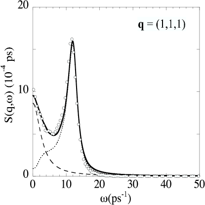
Figure 3: Same as Fig. 2 but for $q=0.21009$ a${}_{0}^{-1}$.

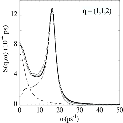
Figure 4: Same as Fig. 2 but for $q=0.29711$ a${}_{0}^{-1}$.

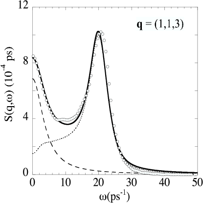
Figure 5: Same as Fig. 2 but for $q=0.40029$ a${}_{0}^{-1}$.

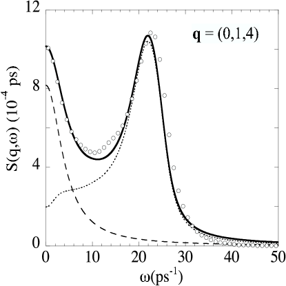
Figure 6: Same as Fig. 2 but for $q=0.50011$ a${}_{0}^{-1}$.

Figure 7: Same as Fig. 2 but for $q=0.70726$ a${}_{0}^{-1}$.

Figure 8: Same as Fig. 2 but for $q=0.81367$ a${}_{0}^{-1}$.

Experience with inelastic neutron scattering in crystals suggests that multimode scattering should become significant at temperatures close to melting and $q$ beyond the first Brillouin zone boundary. This includes our system at $q\gtrsim 0.70$ a${}_{0}^{-1}$. We note that $F_{vib}(q,\infty)$, Eq. (6), is not affected by the one-mode approximation. Since $F_{vib}(q,0)$ is the maximum magnitude of $F_{vib}(q,t)$, an estimate of the accuracy of the one-mode approximation is provided by the ratio $F_{vib}^{(1)}(q,0)/F_{vib}(q,0)$, where the numerator is the one-mode approximation and the denominator is exact. The ratio is listed for each $q$ in Table I. We interpret the results as follows. Multimode scattering, not included in Eq. (17) for $S_{B}(q,\omega)$, is present in the MD data, is small for $q\lesssim 0.50$ a${}_{0}^{-1}$, but is responsible for the discrepancy between model and MD around the Brillouin peak in Figs. 7 and 8.

Let us now consider the magnitude of the fitted parameters. The Rayleigh peak strength $C(q)$, listed in Table I, is greater than 1 and increases steadily as $q$ increases. This implies a considerable cross section for inelastic transit scattering. The Rayleigh peak relaxation rate $\alpha_{1}(q)$ is graphed in Fig. 9. From Eq. (16), $\alpha_{1}(q)$ is the Rayleigh peak half width at half max. $\alpha_{1}(q)$ extrapolates toward zero as $q\rightarrow 0$, while $\alpha_{1}(q)$ is roughly constant at $q\gtrsim 0.5$ a${}_{0}^{-1}$. The Brillouin peak relaxation rate $\alpha_{2}(q)$ is also graphed in Fig. 9, and appears to go to zero at $q$ around 0.1 a${}_{0}^{-1}$. Notice $\alpha_{2}(q)$ does not measure the width of the Brillouin peak, but measures its width beyond the natural width. Hence the $\alpha_{2}(q)$ graph suggests that the liquid Brillouin peak has its natural (vibrational only) width at small $q$, at $q\lesssim 0.1$ a${}_{0}^{-1}$ in the present work. Except where the relaxation rates approach zero at small $q$, $\alpha_{1}$ and $\alpha_{2}$ are in the range 1–5 ps^-1, in qualitative agreement with the mean transit rate $\nu\approx 2.5$ ps^-1.

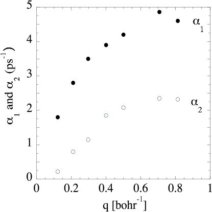
Figure 9: Relaxation rates from our liquid $S(q,\omega)$ model: $\alpha_{1}$ (filled circles) for the Rayleigh peak and $\alpha_{2}$ (empty circles) for the Brillouin peak.

IV Comparison with Mode Coupling Theory

The theory most successful to date in accounting for time correlation functions is mode coupling theory Götze and Lücke (1975). Detailed summaries of mode coupling theories of liquid dynamics are given by Boon and Yip Boon and Yip (1980), Hansen and McDonald Hansen and McDonald (1986), and Balucani and Zoppi Balucani and Zoppi (1994). Mode coupling theory has been applied to the glass transition Bengtzelius et al. (1984); Leutheusser (1984); Götze (1999), and has been shown capable of rationalizing the density correlation functions at temperatures in the vicinity of the glass transition Kob and Andersen (1994, 1995a, 1995b). The application for which we shall compare mode coupling and V-T theories is dynamic response of monatomic liquids at temperatures near and above melting.

Mode coupling theory works with the generalized Langevin equation for $F(q,t)$, and expresses the memory function in terms of processes through which density fluctuations decay Boon and Yip (1980); Hansen and McDonald (1986); Balucani and Zoppi (1994). In the viscoelastic approximation, the memory function decays with a $q$-dependent relaxation time Boon and Yip (1980); Hansen and McDonald (1986); Balucani and Zoppi (1994). This approximation provides a good fit to the combined experimental data Copley and Rowe (1974) and MD data Rahman (1974a, b) for the Brillouin peak dispersion curve in liquid Rb Copley and Lovesey (1975) (see also Fig. 9.2 of Hansen and McDonald (1986)). Going beyond the viscoelastic approximation, Bosse et al Bosse et al. (1978a, b) constructed a self-consistent theory for the longitudinal and transverse current fluctuation spectra, each expressed in terms of relaxation kernels approximated by decay integrals which couple the longitudinal and transverse excitations. This theory is in good overall agreement with extensive neutron scattering data and MD calculations for Ar near its triple point Bosse et al. (1978b). The theory was developed further by Sjögren Sjögren (1980a, b), who separated the memory function into a binary collision part, approximated with a Gaussian ansatz, and a more collective tail represented by a mode coupling term. For liquid Rb, this theory gives an “almost quantitative” agreement with results from neutron scattering experiments Copley and Rowe (1974) and MD calculations Rahman (1974a, b). More recently, inelastic x-ray scattering measurements have been done for the light alkali metals Li Scopigno et al. (2000a) and Na Scopigno et al. (2002a); Yulmetyev et al. (2003). These data have been analyzed by mode coupling theory, and the resulting fits to $S(q,\omega)$ are excellent, both for the experimental data and for MD calculations Scopigno et al. (2002a, b, c, 2000b, 2000c).

A detailed comparison of the present study with the analysis of Scopigno et al. Scopigno et al. (2002a) is of interest. They analyzed experimental data for liquid sodium at 390 K, for $q$ in the range 0.08–0.77 a${}_{0}^{-1}$. Their memory function has three relaxation terms, one for coupling between thermal and density degrees of freedom, with no adjustable parameters, and two for true viscous processes, each having adjustable weight and relaxation time. One parameter is fixed by the total weight, so Scopigno et al. have effectively three $q$-dependent parameters to fit the shape of $S(q,\omega)$. In the present work, we calibrate V-T theory by comparison with MD data for liquid sodium at 395 K, for $q$ in the range 0.12–0.81 a${}_{0}^{-1}$. Our Rayleigh peak contribution has one weight parameter and one relaxation rate, and our Brillouin peak contribution has one relaxation rate, making three adjustable $q$-dependent parameters. Our Brillouin peak weight parameter was fixed at one because we had already confirmed that the vibrational contribution alone has the correct weight. We find that our $\alpha_{1}$ is nearly the same as Scopigno et al.’s inverse relaxation time $\tau_{\alpha}^{-1}$ over the entire $q$ range: the relative difference in magnitude averages 25$\%$. Though we understand the reason, that in each case the parameter is determined by the width of the Rayleigh peak, the level of agreement is remarkable nevertheless. On the other hand, our $\alpha_{2}$ is much smaller than their $\tau_{\mu}^{-1}$, as the ratio $\alpha_{2}/\tau_{\mu}^{-1}$ varies from 0.01 at small $q$ to 0.07 at large $q$. Again the reason is clear: while $\tau_{\mu}^{-1}$ is determined by the Brillouin peak width, $\alpha_{2}$ is determined by only the width beyond the natural width. The result illustrates the important point of comparison between V-T and mode coupling theories: the two methods are based on different decompositions of the physical processes involved. While mode coupling theory analyzes $F(q,t)$ in terms of processes by which density fluctuations decay, V-T theory analyzes $F(q,t)$ in terms of the two contributions to the total liquid motion, vibrations and transits.

V Conclusions

By resolving the complete atomic motion into its constituents, vibrations and transits, V-T theory offers a unified theoretical formulation of equilibrium statistical mechanics averages, both of thermodynamic variables and of time correlation functions. The vibrations alone provide a tractable, accurate, parameter free formulation of thermodynamic properties of monatomic liquids Wallace (1997). The role of transits is merely to allow the liquid to visit the vast array of random valleys, and hence achieve the full liquid entropy Wallace (1997); Chisolm and Wallace (2001); Wallace (2002). The same vibrations provide a tractable, parameter free contribution to time correlation functions, while the same transits, which are part of the equilibrium fluctuations, complete the formulation of time correlation functions.

Our study of the dynamic structure factor exemplifies this unification. The vibrational contribution provides the nontrivial results in Eqs. (8-10) for $S_{vib}(q,\omega)$. Pure elastic scattering is given by $F_{vib}(q,\infty)\;\delta(\omega)$, where $F_{vib}(q,\infty)$ is the positive long-time limit of $F_{vib}(q,t)$. Inelastic scattering in the one-mode approximation is given by $S_{vib}^{(1)}(q,\omega)$, a sum over independent normal-mode cross sections. $S_{vib}^{(1)}(q,\omega)$ provides the natural width of the Brillouin peak Wallace et al. . For liquid sodium at melt, $S_{vib}^{(1)}(q,\omega)$ gives a highly accurate account of the location of the Brillouin peak Wallace et al. , and as we have seen in the present study, gives an accurate account of the Brillouin peak area as well.

As shown in Sec. II, transits contribute to $F_{liq}(q,t)$ in two ways. Transit-induced jumps in the atomic equilibrium positions and displacements cause decorrelation among the terms in Eq. (11), hence transits enhance the decay of time correlations. Transits also provide an additional source of inelastic scattering, hence increase the inelastic cross section. These effects are modeled by the strength parameter $C(q)$ and the relaxation function $e^{-\alpha_{1}(q)\;t}$ in Eq. (13) for $F_{R}(q,t)$, and by the relaxation function $e^{-\alpha_{2}(q)\;t}$ in Eq. (14) for $F_{B}(q,t)$. The model so constructed is a generalization of Zwanzig’s model for the velocity autocorrelation function Zwanzig (1983). The model expressions for $S_{liq}(q,\omega)$ are given in Eqs. (15-17).

As shown in Figs. 2-8, the model can be made to fit MD calculations of $S(q,\omega)$ extremely well, almost within computational errors, except for the two largest $q$ values. The small inadequacy of the model in the vicinity of the Brillouin peak in Figs. 7 and 8 is apparently due to multimode scattering, present in the MD calculation but not in the vibrational theory evaluated here. Properties of the fitting parameters are as follows. In the Rayleigh peak contribution, $C(q)$ is greater than one (Table I), indicating the presence of inelastic transit scattering in the MD calculations. The relaxation rate $\alpha_{1}(q)$ is close to the mean transit rate of 2.5 ps^-1 as expected (Fig. 9), but the figure suggests that $\alpha_{1}(q)$ approaches zero as $q\rightarrow 0$. The Brillouin peak relaxation rate $\alpha_{2}(q)$ appears to vanish at small $q$ (Fig. 9), which would mean that the Brillouin peak width in the liquid is the natural width at small $q$.

Finally, while mode coupling theory and V-T theory each provide a physically based model capable of accurately fitting $S(q,\omega)$ for the liquid at melt, the two models work with entirely different projections of the underlying liquid motion. V-T theory is the more universal, in that it applies the same motional constituents to all statistical averages, equilibrium and nonequilibrium alike.