Tunneling through nanosystems: Combining broadening with many-particle states

Abstract

We suggest a new approach for transport through finite systems based on the Liouville equation. By working in a basis of many-particle states for the finite system, Coulomb interactions are taken fully into account and correlated transitions by up to two different contact states are included. This latter extends standard rate equation models by including level-broadening effects. The main result of the paper is a general expression for the elements of the density matrix of the finite size system, which can be applied whenever the eigenstates and the couplings to the leads are known. The approach works for arbitrary bias and for temperatures above the Kondo temperature. We apply the approach to standard models and good agreement with other methods in their respective regime of validity is found.

I Introduction

Transport through nanosystems such as quantum dots and molecules has received enormous interest within the last decade Datta (1995); Ferry and Goodnick (1997); Imry (2001). Typically this problem is treated within one of two different approximations: (i) Rate equations Beenakker (1991) for electrons entering and leaving the system, which can also take into account complex many-particle states in the central region Kinaret et al. (1992); Pfannkuche and Ulloa (1995). Here broadening effects of the levels are entirely neglected. It can be shown that these rate equations become exact in the limit of high bias Gurvitz and Prager (1996). (ii) The transmission formalism, which is usually evaluated by Green function techniques Meir and Wingreen (1992); Haug and Jauho (1996) (alternatively, scattering states can be calculated directly Frensley (1990)), allows for a consistent treatment of level broadening due to the coupling to the contacts. In principle, many-particle effects can be incorporated into this formalism, but the determination of the appropriate self-energies is a difficult task, where no general scheme has been found by now. Thus, many-particle effects are usually considered on a mean-field basis including exchange and correlation potentials Di Ventra and Lang (2002); Brandbyge et al. (2002); Xue et al. (2002); P.Havu et al. (2004), which are of particular importance for the transport through molecules. Mean-field calculations are well justified for extended systems, such as double-barrier tunneling diodes Pötz (1989); Laux et al. (2004), which exhibit many degrees of freedom (e.g., in the plane perpendicular to the transport). However, the bistability frequently obtained for such structures is questionable for systems with very few degrees of freedom as studied here. See, e.g., the discussion in Sec. III.B.4 of Ref. Sprekeler et al., 2004.

In our paper we want to bridge the gap between these approaches by considering the Liouville equation for the dynamics of the central region coupled to the contacts. The approach works within a basis of arbitrary many-particle states, thus fully taking into account the interactions within the central region. While the first order in the coupling reproduces previous work using rate equations Gurvitz (1998), the second order consistently takes into account broadening effects. This is analogous to the consistent treatment of broadening for tunneling resonances in density-matrix theory. Wacker (2001)

The paper is organized as follows: We first present the formalism in section II. Then we demonstrate its application to the simple problem of tunneling through a single level, section III. We show explicitly that the exact Green function result is recovered for all biases and temperatures. In sections IV we give results for the double-dot system with Coulomb interaction where both standard approaches fail. Finally we consider the spin-degenerate single dot in section V to investigate Coulomb blockade as well as the limit of low temperatures.

II Introducing the formalism

The total Hamiltonian for the system consisting of leads and the dot can be written as

$$H=H_{D}+H_{\text{Leads}}+H_{T}.$$ (1)

The first term describes the dot. Our key issue is the assumption that the dot can be diagonalized in absence of coupling, and the (many-particle) eigenstates and eigenenergies for $H_{D}$ are denoted $|a\rangle$ and $E_{a}$. Thus we have

$$H_{D}=\sum_{a}E_{a}|a\rangle\langle a|.$$ (2)

The leads are described by free-particle states

$$H_{\mathrm{Leads}}=\sum_{k\sigma\ell}E_{k\sigma\ell}c^{\dagger}_{k\sigma\ell}c_{k\sigma\ell}$$ (3)

where $\sigma=\uparrow,\downarrow$ describes the spin, $k$ labels the spatial wave functions of the contact states and $\ell$ denotes the lead. In the following we assume two leads, i.e. $\ell=L,R$, but generalization to more leads is straightforward. Finally, the last part in the Hamiltonian expresses the tunneling between the states in the leads and the dot

$$H_{T}=\sum_{k\sigma\ell,ab}\left[T_{ba}(k\sigma\ell)|b\rangle\!\langle a|c_{k\sigma\ell}+c^{\dagger}_{k\sigma\ell}|a\rangle\!\langle b|T_{ba}^{*}(k\sigma\ell)\right].$$ (4)

The matrix element $T_{ba}(k\sigma\ell)$ is the scattering amplitude for an electron in the state $k\sigma\ell$ tunneling from the lead onto the dot, thereby changing the dot state from state $|a\rangle$ to a state $|b\rangle$. Their evaluation is sketched in App. A. Note that this amplitude vanishes unless the number of electrons in state $|b\rangle$, $N_{b}$, equals $N_{a}+1$. We will generally denote states such that the particle number increases with the position in the alphabet of the denoting letter.

Before proceeding it is important to introduce a consistent notation in order to keep track of the many-particle states in the leads. A general state vector for the entire system is written as $|ag\rangle=|a\rangle\otimes|g\rangle$, with $|g\rangle=|\{N_{k\ell\sigma}\}\rangle$ denoting the state of both leads where $N_{k\sigma\ell}\in\{0,1\}$. Throughout the derivation of the general equations we use the following notation to ensure the anti-commutator rules of the operators

• $|g-k\sigma\ell\rangle\equiv c_{k\sigma\ell}|g\rangle$ and $|g+k\sigma\ell\rangle\equiv c^{\dagger}_{k\sigma\ell}|g\rangle$.
  I.e. $|g-k\sigma\ell\rangle$ denotes the same set of indices as the state $|g\rangle$, but with $N_{k\sigma\ell}$ reduced by one. Furthermore it contains a minus sign depending on the number of occupied states to the left of the position $k\sigma\ell$.

• $|gk\sigma\ell\rangle\equiv c^{\dagger}_{k\sigma\ell}c_{k\sigma\ell}|g\rangle$ and $|g\overline{k\sigma\ell}~{}\rangle\equiv c_{k\sigma\ell}c^{\dagger}_{k\sigma\ell}|g\rangle$. I.e., $|gk\sigma\ell\rangle=\delta_{N_{k\sigma\ell},1}|g\rangle$.

• The order of indices is opposite to the order of the operators. E.g. $|g-k^{\prime}\sigma^{\prime}\ell^{\prime}+k\sigma\ell\rangle=c^{\dagger}_{k\sigma\ell}c_{k^{\prime}\sigma^{\prime}\ell^{\prime}}|g\rangle=-c_{k^{\prime}\sigma^{\prime}\ell^{\prime}}c^{\dagger}_{k\sigma\ell}|g\rangle=-|g+k\sigma\ell-k^{\prime}\sigma^{\prime}\ell^{\prime}\rangle$ for $k\sigma\ell\neq k^{\prime}\sigma^{\prime}\ell^{\prime}$, which is tacitly assumed, unless stated otherwise.

To simplify the notation, $\sigma\ell$ is only attached to $k$ the first time the index $k$ appears in the equation, and in the following it is implicitly assumed to be connected with $k$. We also use the convention that $\sum_{k\sigma(\ell)}$ means summing over $k$ and $\sigma$ with a fixed $\ell$, which is being connected to $k$ in this sum.

The matrix elements of the density operator $\hat{\rho}$ are denoted $\rho_{ag;bg^{\prime}}=\langle ag|\hat{\rho}|bg^{\prime}\rangle$ and the time evolution of the matrix elements are governed by the von Neumann equation

$${\rm i}\hbar\frac{{\rm d}}{{\rm d}t}\rho_{ag;bg^{\prime}}=\langle ag|H\hat{\rho}-\hat{\rho}H|bg^{\prime}\rangle$$ (5)

The particle current from the left lead into the structure, $J_{L}$, equals the rate of change in the occupation of the left lead. We find that

$$\begin{split}J_{L}&=-\frac{{\rm d}}{{\rm d}t}\sum_{k\sigma(L)}\left\langle c^{\dagger}_{k}c_{k}\right\rangle=-\frac{{\rm d}}{{\rm d}t}\sum_{k\sigma(L)}\rho_{bg,bgk}\\ &=-\frac{2}{\hbar}\sum_{k\sigma(L),cb}\Im\left\{\sum_{g}T^{*}_{cb}(k)\rho_{cg-k;bg}\right\}\end{split}$$ (6)

where we have used the definition of the density operator to calculate the average value of the number operator in the left lead.

The goal is to determine these elements of the density matrix, which describe the correlations between the leads and the dot. They are determined using the equation-of-motion technique, and from Eq. (5) we obtain

$${\rm i}\hbar\frac{{\rm d}}{{\rm d}t}\rho_{cg-k\sigma\ell;bg}=(E_{c}-E_{b}-E_{k})\rho_{cg-k;bg}\\ +\sum_{b^{\prime}}T_{cb^{\prime}}(k)\rho_{b^{\prime}gk;bg}-\sum_{c^{\prime}}\rho_{cg-k;c^{\prime}g-k}T_{c^{\prime}b}(k)\\ +\sum_{k^{\prime}\sigma^{\prime}\ell^{\prime}}\Big{[}\sum_{b^{\prime}}T_{cb^{\prime}}(k^{\prime})\rho_{b^{\prime}g-k+k^{\prime};bg}+\sum_{d}T_{dc}^{*}(k^{\prime})\rho_{dg-k-k^{\prime};bg}\\ -\sum_{c^{\prime}}\rho_{cg-k;c^{\prime}g-k^{\prime}}T_{c^{\prime}b}(k^{\prime})-\sum_{a}\rho_{cg-k;ag+k^{\prime}}T_{ba}^{*}(k^{\prime})\Big{]}.$$ (7)

While $\rho_{cg-k\sigma\ell;bg}$ describes the transition of an electron with quantum number $k$ and spin $\sigma$ from lead $\ell$ to the central region, terms like $\rho_{b^{\prime}g-k+k^{\prime};bg}$ describe the correlated transition of two electrons with $k$ and $k^{\prime}$. $\rho_{b^{\prime}g-k+k^{\prime};bg}$ satisfies a similar equation of motion containing also correlated transition of three electrons on the right hand side. In order to break the hierarchy we apply three approximations:

(i) We only consider coherent processes involving transitions of at most two different $k$-states. (ii) The time dependence of terms generating two-electron transition processes is neglected, which corresponds to the Markov limit. Kuhn (1998) (iii) We assume that the level occupations $f_{k\sigma\ell}$ in the leads are unaffected by the kinetics of the dot, so it is possible to factorize the density in the leads and on the dot. This is realistic for ”large” leads which are strongly coupled to reservoirs, i.e. good contacts.

Defining

$$w_{b^{\prime}b} = \sum_{g}\rho_{b^{\prime}g;bg},$$ (8)

$$\phi_{ba}(k\sigma\ell) = \sum_{g}\rho_{bg-k;ag}$$ (9)

we find the following set of coupled differential equations (see Appendix B for a detailed derivation):

$$\begin{split}{\rm i}\hbar\frac{{\rm d}}{{\rm d}t}\phi_{cb}(k\sigma\ell)=&(E_{c}-E_{b}-E_{k})\phi_{cb}(k)+\sum_{b^{\prime}}T_{cb^{\prime}}(k)f_{k}w_{b^{\prime}b}-\sum_{c^{\prime}}(1-f_{k})w_{cc^{\prime}}T_{c^{\prime}b}(k)\\ +&\sum_{a,b^{\prime},k^{\prime}\sigma^{\prime}\ell^{\prime}}\frac{\left[T_{cb^{\prime}}(k^{\prime})f_{k^{\prime}}\phi_{b^{\prime}a}(k)-(1-f_{k})\phi_{cb^{\prime}}(k^{\prime})T_{b^{\prime}a}(k)\right]T_{ba}^{*}(k^{\prime})}{E_{k}+E_{k^{\prime}}-(E_{c}-E_{a})+{\rm i}0^{+}}\\ +&\sum_{a,b^{\prime},k^{\prime}\sigma^{\prime}\ell^{\prime}}\frac{\left[(1-f_{k^{\prime}})\phi_{cb^{\prime}}(k)T_{b^{\prime}a}(k^{\prime})-T_{cb^{\prime}}(k)f_{k}\phi_{b^{\prime}a}(k^{\prime})\right]T_{ba}^{*}(k^{\prime})}{E_{k}+E_{k^{\prime}}-(E_{c}-E_{a})+{\rm i}0^{+}}\\ +&\sum_{a,b^{\prime},k^{\prime}\sigma^{\prime}\ell^{\prime}}\frac{T_{cb^{\prime}}(k^{\prime})\left[f_{k^{\prime}}\phi_{b^{\prime}a}(k)T_{ba}^{*}(k^{\prime})-T_{b^{\prime}a}(k)f_{k}\phi_{ba}^{*}(k^{\prime})\right]}{E_{k}-E_{k^{\prime}}-(E_{b^{\prime}}-E_{b})+{\rm i}0^{+}}\\ +&\sum_{b^{\prime},c^{\prime},k^{\prime}\sigma^{\prime}\ell^{\prime}}\frac{T_{cb^{\prime}}(k^{\prime})\left[T^{*}_{c^{\prime}b^{\prime}}(k^{\prime})(1-f_{k^{\prime}})\phi_{c^{\prime}b}(k)-(1-f_{k})\phi^{*}_{c^{\prime}b^{\prime}}(k^{\prime})T_{c^{\prime}b}(k)\right]}{E_{k}-E_{k^{\prime}}-(E_{b^{\prime}}-E_{b})+{\rm i}0^{+}}\\ +&\sum_{b^{\prime},c^{\prime},k^{\prime}\sigma^{\prime}\ell^{\prime}}\frac{\left[f_{k^{\prime}}\phi_{cb^{\prime}}(k)T_{c^{\prime}b^{\prime}}^{*}(k^{\prime})-T_{cb^{\prime}}(k)f_{k}\phi_{c^{\prime}b^{\prime}}^{*}(k^{\prime})\right]T_{c^{\prime}b}(k^{\prime})}{E_{k}-E_{k^{\prime}}-(E_{c}-E_{c^{\prime}})+{\rm i}0^{+}}\\ +&\sum_{c^{\prime},d,k^{\prime}\sigma^{\prime}\ell^{\prime}}\frac{\left[T_{dc}^{*}(k^{\prime})(1-f_{k^{\prime}})\phi_{dc^{\prime}}(k)-(1-f_{k})\phi^{*}_{dc}(k^{\prime})T_{dc^{\prime}}(k)\right]T_{c^{\prime}b}(k^{\prime})}{E_{k}-E_{k^{\prime}}-(E_{c}-E_{c^{\prime}})+{\rm i}0^{+}}\\ +&\sum_{c^{\prime},d,k^{\prime}\sigma^{\prime}\ell^{\prime}}\frac{T_{dc}^{*}(k^{\prime})\left[(1-f_{k^{\prime}})\phi_{dc^{\prime}}(k)T_{c^{\prime}b}(k^{\prime})-T_{dc^{\prime}}(k)f_{k}\phi_{c^{\prime}b}(k^{\prime})\right]}{E_{k}+E_{k^{\prime}}-(E_{d}-E_{b})+{\rm i}0^{+}}\\ +&\sum_{c^{\prime},d,k^{\prime}\sigma^{\prime}\ell^{\prime}}\frac{T_{dc}^{*}(k^{\prime})\left[T_{dc^{\prime}}(k^{\prime})f_{k^{\prime}}\phi_{c^{\prime}b}(k)-(1-f_{k})\phi_{dc^{\prime}}(k^{\prime})T_{c^{\prime}b}(k)\right]}{E_{k}+E_{k^{\prime}}-(E_{d}-E_{b})+{\rm i}0^{+}}\end{split}$$ (10)

$${\rm i}\hbar\frac{{\rm d}}{{\rm d}t}w_{bb^{\prime}}=(E_{b}-E_{b^{\prime}})w_{bb^{\prime}}+\sum_{a,k\sigma\ell}\left(T_{ba}(k)\phi^{*}_{b^{\prime}a}(k)-\phi_{ba}(k)T^{*}_{b^{\prime}a}(k)\right)+\sum_{c,k\sigma\ell}\left(T_{cb}^{*}(k)\phi_{cb^{\prime}}(k)-\phi^{*}_{cb}(k)T_{cb^{\prime}}(k)\right)$$ (11)

These equations are the main result of this paper. They satisfy current conservation, as shown in App. C. The numerical implementation of this approach is straightforward and we will give examples in the following sections.

If we entirely neglect the correlated two-particle transitions, only the first line of Eq. (10) remains. Applying the Markov limit we obtain a set of equations analogously to Eqs. (2a,b) of Ref. Gurvitz, 1998. This shows that our approximation scheme goes substantially beyond the rate equation scheme of Gurvitz Gurvitz (1998), which only holds in the high-bias limit.

III Single level without spin

In order to demonstrate the formalism described in the previous section we consider a single level without spin. We show that this case can be solved analytically in the stationary state and that the exact nonequilibrium Green function result is recovered.

The possible dot states are the empty state $0$ with energy $E_{0}=0$ and the occupied state $1$ with energy $E_{1}$. The coupling matrix elements between the leads and the dot are $T_{10}(k\ell)=T_{\ell}(k)$, and the others equal zero.
Inserting this in Eq. (10) with $c=1$ and $b=0$ gives

$$\begin{split}{\rm i}\hbar\frac{{\rm d}}{{\rm d}t}&\phi_{10}(k\ell)=\left[E_{1}-E_{k}+\Sigma(E_{k})\right]\phi_{10}(k\ell)\\ &-T_{\ell}(k)\sum_{k^{\prime}\ell^{\prime}}\frac{T_{\ell^{\prime}}(k^{\prime})\phi^{*}_{10}(k^{\prime}\ell^{\prime})}{E_{k}-E_{k}^{\prime}+{\rm i}0^{+}}+T_{\ell}(k)(f_{k}-w_{11}),\end{split}$$ (12)

where the self-energy

$$\Sigma(E)=\sum_{k\ell}\frac{|T_{\ell}(k)|^{2}}{E-E_{k}+{\rm i}0^{+}}$$ (13)

has been introduced, and we have used the normalization of the probability $w_{00}+w_{11}=1$.

After multiplying Eq. (12) with $T_{\ell}^{*}(k)\delta(E-E_{k})$ and summing over all $k$-states (in a fixed lead $\ell$) we obtain

$$\begin{split}{\rm i}\hbar&\frac{{\rm d}}{{\rm d}t}B^{\ell}_{10}(E)=\left[E_{1}-E+\Sigma(E)\right]B^{\ell}_{10}(E)\\ &-\frac{\Gamma_{\ell}(E)}{2\pi}\int{\rm d}E^{\prime}\frac{B_{10}^{L*}(E^{\prime})+B_{10}^{R*}(E^{\prime})}{E-E^{\prime}+{\rm i}0^{+}}\\ &+\frac{\Gamma_{\ell}(E)}{2\pi}[f_{\ell}(E)-w_{11}]\end{split}$$ (14)

for the new variable

$$B^{\ell}_{10}(E)=\sum_{k}\delta(E-E_{k})T_{\ell}^{*}(k)\phi_{10}(k\ell)$$ (15)

where $\Gamma_{\ell}(E)=2\pi\sum_{k}\delta(E-E_{k})|T_{\ell}(k)|^{2}$.
Eq. (11) becomes

$$\frac{{\rm d}}{{\rm d}t}w_{11}=-\frac{2}{\hbar}\int{\rm d}E\,\Im\left\{B^{L}_{10}(E)+B^{R}_{10}(E)\right\}\,.$$ (16)

Finally, the current formula Eq. (6) yields

$$J_{L}=-\frac{2}{\hbar}\int{\rm d}E~{}\Im\left\{B^{L}_{10}(E)\right\}\,.$$ (17)

Throughout this paper, we apply Fermi functions $f_{k\sigma\ell}=1/[\exp((E_{k}-\mu_{\ell})/k_{B}T)+1]\equiv f_{\ell}(E_{k})$ for the lead occupations with chemical potentials $\mu_{\ell}$ and temperature $T$. Except for this section, the bias $V$ is applied symmetrically around zero, i.e. $\mu_{L}=V/2$, $\mu_{R}=-V/2$. The contact functions $\Gamma_{\ell}(E)$ are assumed to be zero for $|E|>W$, while they take the constant values $\Gamma_{\ell}$, independent of spin, for $|E|<0.95W$. For $0.95W<|E|<W$ we interpolate with an elliptic behavior in order to avoid discontinuities.

The time-dependent net-current $J_{R}(t)$ flowing from the right lead into the single level has been calculated from Eqs. (14,16,17) in the following situation: For times $t<0$ the chemical potentials of both leads and the single level are aligned, i.e. $\mu_{L}^{0}=\mu_{R}^{0}=E_{1}=0$. At $t=0$ the chemical potential of the left lead is raised instantaneously to $\mu_{L}$ giving a step-like modulation of the bias. The result is shown for different values of $\mu_{L}$ in Fig. 1. Also shown is the result of an exact time-dependent Green function calculation.Stefanucci and Almbladh (2004) It is not surprising that our results do not show the exact time-dependence because the Markov limit has been invoked in the derivation of the generalized equation system in Eqs. (10,11).

In the long-time limit, we reach a stationary state with the current

$$J_{L}=J_{R}=\frac{1}{\hbar}\int\frac{{\rm d}E}{2\pi}\frac{\Gamma_{L}(E)\Gamma_{R}(E)[f_{L}(E)-f_{R}(E)]}{|E-E_{1}-\Sigma(E)|^{2}},$$ (18)

which is derived analytically in App. D. Eq. (18) is in full agreement with the exact nonequilibrium Green function result. Meir and Wingreen (1992)

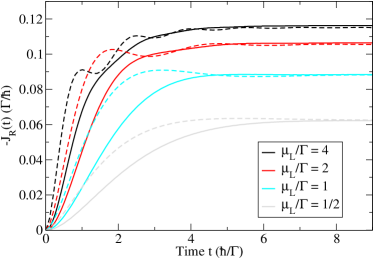
Figure 1: (Color online) The time-dependent current calculated with our method (full line) and with the time-dependent Green function method from Ref. Stefanucci and Almbladh, 2004 (dashed line) as response to a step-like modulation of the bias with step height $\mu_{L}$. The coupling is $\Gamma_{L}=\Gamma_{R}=\Gamma/2$, the temperature $k_{B}T=0.05\Gamma$, and the half-width of the band is $W=30\Gamma$.

IV Double quantum dot

The double quantum dot structure, where the dots are coupled in series, is a standard example to study tunneling through a multiple-level system. In case of Coulomb interaction and finite bias the validity of both the rate equation method and the Green function formalism is limited.

To simplify the analysis we treat the spinless case. (A possible realization is to favor one spin polarization of the electron by a high magnetic field.) Denoting the left/right dot by $\alpha/\beta$, the Hamiltonian reads

$$\begin{split}H=&E_{\alpha}d_{\alpha}^{\dagger}d_{\alpha}+E_{\beta}d_{\beta}^{\dagger}d_{\beta}+Ud_{\alpha}^{\dagger}d_{\alpha}d_{\beta}^{\dagger}d_{\beta}\\ &+\left(\Omega d_{\beta}^{\dagger}d_{\alpha}+h.c\right)+\sum_{k\ell}E_{k\ell}c^{\dagger}_{k\ell}c_{k\ell}\\ &+\sum_{k}\Big{(}t_{kL}d_{\alpha}^{\dagger}c_{kL}+t_{kR}d_{\beta}^{{{\dagger}}}c_{kR}+h.c.\Big{)}\end{split}$$ (19)

with $\Omega$ being the interdot tunneling coupling and $U$ the Coulomb energy for occupying both dots. The first four terms describe the isolated double quantum dot $H_{D}$. Diagonalizing this part of the Hamiltonian gives the following states

$$|0\rangle =|0\rangle, E_{0} =0,$$

$$|1\rangle =(\alpha_{1}d_{\alpha}^{{\dagger}}+\beta_{1}d_{\beta}^{{\dagger}})|0\rangle, \quad E_{1} =\frac{1}{2}\left[\rho-\sqrt{\Delta^{2}+4\Omega^{2}}\right],$$

$$|2\rangle =(\alpha_{2}d_{\alpha}^{{\dagger}}+\beta_{2}d_{\beta}^{{\dagger}})|0\rangle, \quad E_{2} =\frac{1}{2}\left[\rho+\sqrt{\Delta^{2}+4\Omega^{2}}\right],$$

$$|d\rangle =d_{\alpha}^{{\dagger}}d_{\beta}^{{\dagger}}|0\rangle, E_{d} =E_{\alpha}+E_{\beta}+U,$$

with $\Delta=E_{\alpha}-E_{\beta}$, $\rho=E_{\alpha}+E_{\beta}$, $C_{\pm}=\frac{\Delta\pm\sqrt{\Delta^{2}+4\Omega^{2}}}{2\Omega}$, $\alpha_{1/2}=\frac{C_{\mp}}{\sqrt{1+C^{2}_{\mp}}}$ and $\beta_{1/2}=\frac{1}{\sqrt{1+C^{2}_{\mp}}}$.

From Appendix A we find

$$\begin{split}H_{T}=&\sum_{k\ell}\Big{[}T_{10}^{\ell}(k)|1\rangle\langle 0|c_{k{\ell}}+T_{20}^{\ell}(k)|2\rangle\langle 0|c_{k{\ell}}\\ &+T_{d1}^{\ell}(k)|d\rangle\langle 1|c_{k{\ell}}+T_{d2}^{\ell}(k)|d\rangle\langle 2|c_{k{\ell}}\Big{]}+h.c.\end{split}$$ (20)

with (skipping the k-dependence of the matrix elements)

$$T_{10}^{L} =t_{L}^{*}\langle 1|d_{\alpha}^{{\dagger}}|0\rangle=t_{L}^{*}\alpha_{1}^{*}, T_{20}^{L} =t_{L}^{*}\langle 2|d_{\alpha}^{{\dagger}}|0\rangle=t_{L}^{*}\alpha_{2}^{*},$$

$$T_{10}^{R} =t_{R}^{*}\langle 1|d_{\beta}^{{\dagger}}|0\rangle=t_{R}^{*}\beta_{1}^{*}, T_{20}^{R} =t_{R}^{*}\langle 2|d_{\beta}^{{\dagger}}|0\rangle=t_{R}^{*}\beta_{2}^{*},$$

$$T_{d1}^{L} =t_{L}^{*}\langle d|d_{\alpha}^{{\dagger}}|1\rangle=t_{L}^{*}\beta_{1}, T_{d2}^{L} =t_{L}^{*}\langle d|d_{\alpha}^{{\dagger}}|2\rangle=t_{L}^{*}\beta_{2},$$

$$T_{d1}^{R} =t_{R}^{*}\langle d|d_{\beta}^{{\dagger}}|1\rangle=-t_{R}^{*}\alpha_{1}, \quad T_{d2}^{R} =t_{R}^{*}\langle d|d_{\beta}^{{\dagger}}|2\rangle=-t_{R}^{*}\alpha_{2},$$

where the signs of the coupling matrix elements are due to the order of the operators in the double-occupied state.

Applying the method in the same way as for the single level system gives eight different functions of the type $B^{\ell}_{cb}(E)$ and five different occupations $\omega_{bb^{\prime}}$. These equations have been solved and the stationary current has been recorded.

By comparing with exact Green function results, it has been verified numerically that in the non-interacting case ($U=0$) the exact transmission is obtained for various values of level splitting and interdot coupling (not shown). Furthermore, for both $U=0$ and non-zero $U$ we have calculated the stationary current in a situation where the levels are de-aligned with $E_{\alpha}=-E_{\beta}=0.5\Gamma$, and $\Omega=\Gamma$. The results for different values of $U$ are shown in Fig. 2 together with the Green function result for $U=0$. Obviously, the latter is fully recovered in the non-interacting limit. The straight dashed line in the figure is the quantum rate equation result obtained by Stoof and NazarovStoof and Nazarov (1996), which is valid in the high-bias limit ($V\to\infty$) for $U\rightarrow\infty$. The same result is found in Ref. Gurvitz and Prager, 1996 using another rate equation method. The small discrepancy between the results could be due to the finite bandwidth used in our calculation. For intermediate values of $U$ the results looks reasonable and exhibit a smooth interpolation between the limiting cases. The kink on the curve for finite $U$ is due to the single occupied state.

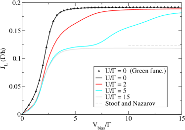
Figure 2: (Color online) Stationary current through the double quantum dot structure for different values of the interdot Coulomb repulsion $U$. The triangles are from a nonequilibrium Green function calculation, and the dotted line is the result by Stoof and Nazarov Stoof and Nazarov (1996) valid in high-bias limit for $U\rightarrow\infty$. The levels of the dot are placed symmetrically around the zero-bias with $E_{\alpha}-E_{\beta}=\Gamma$. We use the interdot tunneling coupling $\Omega=\Gamma$, $\Gamma_{L}=\Gamma_{R}=\Gamma/2$, the temperature $k_{B}T=0.1\Gamma$, and the half-width of the band $W=20\Gamma$.

V Spin-degenerate level

Now we consider a spin-degenerate single level with energy $E_{1}$ and Coulomb interaction $U$. We use the parameters $U=1.9$ meV, and $\Gamma=\Gamma_{L}+\Gamma_{R}=0.295$ meV, as experimentally determined for the structure studied in Ref. Goldhaber-Gordon et al., 1998. The conductance

$$G=e^{2}\frac{{\rm d}J}{{\rm d}(\mu_{L}-\mu_{R})}$$ (21)

is expected to reach $G_{0}=\frac{e^{2}}{h}\,8\Gamma_{L}\Gamma_{R}/(\Gamma_{L}+\Gamma_{R})^{2}$ in the zero-bias limit $\mu_{L}\to\mu_{R}$ for temperatures far below the Kondo temperature $T_{K}$ Ng and Lee (1988); Glazman and Raikh (1988). As $G_{\rm max}\approx 0.5e^{2}/h$ in the experiment we use $\Gamma_{L}=0.275$ meV and $\Gamma_{R}=0.02$ meV. Furthermore the band width $W=5$ meV is applied. In Fig. 3 we show the zero-bias conductance as a function of the dot level, which is modified by a gate bias in the experiment. We find the standard Coulomb oscillations, where the conductance exhibits peaks whenever the single-particle excitation energies are close to the Fermi edge of the contacts, $\mu=0$ (depicted by vertical dashed lines at $E_{1}=0$ and $E_{1}=-U$). The peak positions and widths are in good agreement with the data given in Fig. 2 of Ref. Goldhaber-Gordon et al., 1998. The peak heights for the peak around $E_{1}\approx 0$ agree reasonably with the experiment, if one takes into account that for elevated temperatures the presence of different levels raise the conductance which is not included in our single-level model. (The experimental level spacing corresponds to 5 K.) The experimental peak heights for the peak at $E_{1}\approx-U$ are lower, while they are exactly identical with the corresponding peaks $E_{1}\approx 0$ due to electron-hole symmetry in our calculation. Possible sources for this deviation result from an energy-dependence of the $\Gamma_{\ell}(E)$ in the experiment or the admixture of different levels.

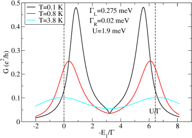
Figure 3: (Color online) Zero-bias conductance as a function of level position for different temperatures. All parameters are according to the experimental data shown in Fig. 2 of Ref. Goldhaber-Gordon et al., 1998.

Further lowering the temperature, the zero-bias conductance should increase in the region $0<E_{1}<U$, due to the Kondo effect Ng and Lee (1988); Glazman and Raikh (1988). Albeit we observe an increase in parts of this region, the (probable unphysical) dip in our curve for $T=0.1$ K at $E_{1}=-U/2$ persists even at lower temperatures. Furthermore the conductance can exceed $G_{0}$ at the peaks. This indicates that our approach fails in the Kondo limit, where strong correlations between lead and dot state require elaborated renormalization group Costi et al. (1994); Schoeller and König (2000); Rosch et al. (2003) or slave boson Wingreen and Meir (1994); Dong and Lei (2001) techniques.

In Fig. 4 we show the finite bias conductance at 0.8 K, where both the conductance peaks for $\mu_{L}\approx\mu_{R}$ discussed above as well as the excitations can be detected. We observe a strong asymmetry due to $\Gamma_{L}\gg\Gamma_{R}$. This can be understood from Fig. 5, where the current is plotted versus bias at the single-electron excitation peak $E_{1}=0$. For negative bias the electrons rapidly leave the dot via the thin left barrier and the dot is essentially empty. Thus both spin directions can tunnel through the thick right barrier, which is limiting the current. In contrast, for positive bias the dot is occupied with a single electron (as long as $\mu_{L}=V/2<E_{1}+U$) with a given spin and only this spin direction may tunnel through the thick barrier, reducing the current approximately by a factor of 2. We have shown the respective results for the rate equation model Gurvitz and Prager (1996) for comparison. The short-dashed horizontal lines refer to a bias which allows only single occupation of the dot, while the long-dashed line considers the case where both the single- and the two-particle state are located between both Fermi levels. The currents from the rate equation model slightly exceed our results, as the peaks are not completely within the bias window due to broadening.

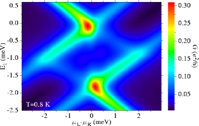
Figure 4: (Color online) Differential conductance for finite bias. Parameters as in Fig. 3.

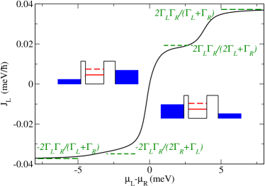
Figure 5: (Color online) Current versus bias for $E_{1}=0$ and $T=0.8$ K. Parameters as in Fig. 3. The dashed horizontal lines correspond to the rate equation model by Gurvitz and PragerGurvitz and Prager (1996), where we added the respective formulae.

VI Discussion and summary

We have presented an approach for transport through finite systems based on the Liouville equation. This approach recovers the results from the Green-function method in the noninteracting limit for the models studied. In the high-bias limit the results are consistent with the many-particle rate equations. Thus it bridges the gap between these approaches and allows for a consistent treatment of Coulomb interaction and broadening effects for arbitrary bias. E.g. Coulomb blockade peaks are correctly reproduced. The model fails below the Kondo temperature where strong correlations between the finite system and the contacts dominate the behavior.

Correlations between tunneling events have been previously studied by the method of a diagrammatic real-time technique König et al. (1997). While this work was completed we also became aware of a cumulant expansion of the tunneling Hamiltonian Li et al. (2005). It would be interesting to study the relation between these approaches and our method. A central question is here, whether the exact Green function result, such as Eq. (18), can be obtained for the noninteracting case.

The numerical implementation of our approach is straightforward and explicit results were presented for standard model systems made by up to two single-particle states. For larger systems the number of many-particle states $b,c$ increases dramatically, and so does the number of $\phi_{bc}$-functions. Thus sophisticated routines are needed for the implementation and evaluation of real systems.

Appendix A Determination of matrix elements $T_{ab}(k)$

Conventually one starts with a single-particle basis in the central region with wave functions $\Psi_{n}({\bf r})$, spin functions $\chi_{\sigma}$ and associated creation operators $d^{{\dagger}}_{n\sigma}$. Then an arbitrary many-particle state $|a\rangle$ can be written as

$$|a\rangle=\sum_{\bf j}a_{\bf j}d^{{\dagger}}_{j_{1}}d^{{\dagger}}_{j_{2}}\ldots d^{{\dagger}}_{j_{N_{a}}}|0\rangle$$

where $j_{i}=n_{i}\sigma_{i}$ determines the $i$-th single-particle state in the $N_{a}$-particle Slater determinant determined by the index set ${\bf j}=(j_{1},j_{2},\ldots j_{N_{a}})$. In order to avoid double counting, we restrict to the ordering $n_{1}\leq n_{2}\leq\ldots\leq n_{N_{a}}$, where spin-up precedes spin-down for equal $n$. The expansion coefficients $a_{\bf j}$ can be obtained by exact diagonalization of the dot Hamiltonian.

In the single-particle basis the tunneling Hamiltonian reads

$$H_{T}=\sum_{k\sigma\ell,n}\left(t^{*}_{n\ell}(k\sigma\ell)c^{{\dagger}}_{k\sigma\ell}d_{n\sigma}+t_{n\ell}(k\sigma\ell)d_{n\sigma}^{{\dagger}}c_{k\sigma\ell}\right)$$ (22)

Inserting the unit operators $\sum_{a}|a\rangle\langle a|$, $\sum_{b}|b\rangle\langle b|$ we find

$$\begin{split}H_{T}=\sum_{k\sigma\ell,a,b}&\Big{(}c^{{\dagger}}_{k\sigma\ell}|b\rangle\underbrace{\sum_{n}t^{*}_{n\ell}(k\sigma\ell)\langle b|d_{n\sigma}|a\rangle}_{=T^{*}_{ab}(k\sigma\ell)}\langle a|\\ &+|a\rangle\underbrace{\sum_{n}t_{n\ell}(k\sigma\ell)\langle a|d^{{\dagger}}_{n\sigma}|b\rangle}_{=T_{ab}(k\sigma\ell)}\langle b|c_{k\sigma\ell}\Big{)}\end{split}$$ (23)

to be used in Eq. (4).

Appendix B Derivation of Eqs. (10,11)

Using the approximation (i) we find for one of the two-electron transition terms in Eq. (7)

$${\rm i}\hbar\frac{{\rm d}}{{\rm d}t}\rho_{b^{\prime}g-k\sigma\ell+k^{\prime}\sigma^{\prime}\ell^{\prime};bg}=(E_{b^{\prime}}+E_{k^{\prime}}-E_{b}-E_{k})\rho_{b^{\prime}g-k+k^{\prime};bg}\\ -\sum_{a}T_{b^{\prime}a}(k)\rho_{agk+k^{\prime};bg}+\sum_{c^{\prime}}T_{c^{\prime}b^{\prime}}^{*}(k^{\prime})\rho_{c^{\prime}g-k\overline{k^{\prime}};bg}\\ -\sum_{c^{\prime}}\rho_{b^{\prime}g-k+k^{\prime};c^{\prime}g-k}T_{c^{\prime}b}(k)-\sum_{a}\rho_{b^{\prime}g-k+k^{\prime};ag+k^{\prime}}T_{ba}^{*}(k^{\prime})$$

Now we take the Markov limit (ii) following the standard treatment of density matrix theory for ultrafast dynamics Kuhn (1998). This implies adding $-{\rm i}0^{+}\rho_{b^{\prime}g-k\sigma\ell+k^{\prime}\sigma^{\prime}\ell^{\prime};bg}$ on the right hand side in order to guaranty the decay of initial conditions at $t=-\infty$, and neglecting the time dependence of the inhomogeneity (second and third line). Then this linear differential equation can be solved directly, yielding

$$\rho_{b^{\prime}g-k\sigma\ell+k^{\prime}\sigma^{\prime}\ell^{\prime};bg}=\frac{1}{E_{k}-E_{k^{\prime}}-(E_{b^{\prime}}-E_{b})+{\rm i}0^{+}}\\ \times\Big{[}-\sum_{a}T_{b^{\prime}a}(k)\rho_{agk+k^{\prime};bg}+\sum_{c^{\prime}}T_{c^{\prime}b^{\prime}}^{*}(k^{\prime})\rho_{c^{\prime}g-k\overline{k^{\prime}};bg}\\ -\sum_{c^{\prime}}\rho_{b^{\prime}g-k+k^{\prime};c^{\prime}g-k}T_{c^{\prime}b}(k)-\sum_{a}\rho_{b^{\prime}g-k+k^{\prime};ag+k^{\prime}}T_{ba}^{*}(k^{\prime})\Big{]}$$

In the same way the other two-electron transition terms in Eq. (7) are determined by

$$\rho_{dg-k\sigma\ell-k^{\prime}\sigma^{\prime}\ell^{\prime};bg}=\frac{1}{E_{k}+E_{k^{\prime}}-(E_{d}-E_{b})+{\rm i}0^{+}}\\ \times\sum_{c^{\prime}}\Big{[}-T_{dc^{\prime}}(k)\rho_{c^{\prime}gk-k^{\prime};bg}+T_{dc^{\prime}}(k^{\prime})\rho_{c^{\prime}g-kk^{\prime};bg}\\ -\rho_{dg-k-k^{\prime};c^{\prime}g-k}T_{c^{\prime}b}(k)-\rho_{dg-k-k^{\prime};c^{\prime}g-k^{\prime}}T_{c^{\prime}b}(k^{\prime})\Big{]},$$

$$\rho_{cg-k\sigma\ell;c^{\prime}g-k^{\prime}\sigma^{\prime}\ell^{\prime}}=\frac{1}{E_{k}-E_{k^{\prime}}-(E_{c}-E_{c^{\prime}})+{\rm i}0^{+}}\\ \times\Big{[}\sum_{b^{\prime}}T_{cb^{\prime}}(k)\rho_{b^{\prime}gk;c^{\prime}g-k^{\prime}}+\sum_{d}T_{dc}^{*}(k^{\prime})\rho_{dg-k-k^{\prime};c^{\prime}g-k^{\prime}}\\ -\sum_{d}\rho_{cg-k;dg-k^{\prime}-k}T_{dc^{\prime}}(k)-\sum_{b^{\prime}}\rho_{cg-k;b^{\prime}gk^{\prime}}T_{c^{\prime}b^{\prime}}^{*}(k^{\prime})\Big{]},$$

$$\rho_{cg-k\sigma\ell;ag+k^{\prime}\sigma^{\prime}\ell^{\prime}}=\frac{1}{E_{k}+E_{k^{\prime}}-(E_{c}-E_{a})+{\rm i}0^{+}}\\ \times\sum_{b^{\prime}}\Big{[}T_{cb^{\prime}}(k)\rho_{b^{\prime}gk;ag+k^{\prime}}+T_{cb^{\prime}}(k^{\prime})\rho_{b^{\prime}g-k+k^{\prime};ag+k^{\prime}}\\ -\rho_{cg-k;b^{\prime}g+k^{\prime}-k}T_{b^{\prime}a}(k)-\rho_{cg-k;b^{\prime}g\overline{k^{\prime}}}T_{b^{\prime}a}(k^{\prime})\Big{]}.$$

In order to obtain Eq. (10) we sum over $g$ in Eq. (7) after inserting the above approximations for the two-electron transition terms. Using the definitions (8,9) and the decoupling assumption (iii) we obtain

$$\sum_{g}\rho_{b^{\prime}gk;bg}=\sum_{g}\delta_{N_{k},1}\rho_{b^{\prime}g;bg}\approx f_{k}\sum_{g}\rho_{b^{\prime}g;bg}=f_{k}w_{b^{\prime}b}$$

Similarly

$$\begin{split}\sum_{g}\rho_{b^{\prime}g\overline{k};bg}&\approx(1-f_{k})w_{b^{\prime}b},\\ \sum_{g}\rho_{bg-k^{\prime}k;ag}&\approx f_{k}\phi_{ba}(k^{\prime}),\\ \sum_{g}\rho_{bg-k^{\prime}\overline{k};ag}&\approx(1-f_{k})\phi_{ba}(k^{\prime})\end{split}$$

Furthermore note that

$$\begin{split}\sum_{g}\rho_{bg;ag+k}=&\sum_{\tilde{g}}\rho_{b\tilde{g}-k;a\tilde{g}}=\phi_{ba}(k)\\ \sum_{g}\rho_{b^{\prime}g+k;bg+k}=&\sum_{\tilde{g}}\rho_{b^{\prime}\tilde{g}k;b\tilde{g}}\approx f_{k}w_{b^{\prime}b}\end{split}$$

as well as similar relations hold, where $|\tilde{g}\rangle$ is identical with $|g\rangle$ except for exchanging 1 and 0 in the occupation of state $k$ (including the appropriate change of sign). Particular care has to be taken in order to insure the anti-commutation rules. E.g., $\sum_{g}\rho_{b^{\prime}g-k+k^{\prime};ag+k^{\prime}}\approx-f_{k^{\prime}}\phi_{b^{\prime}a}(k)$.

In the same way

$$\begin{split}{\rm i}\hbar&\frac{{\rm d}}{{\rm d}t}\rho_{bg;b^{\prime}g}=(E_{b}-E_{b^{\prime}})\rho_{bg;b^{\prime}g}\\ &+\sum_{a,k\sigma\ell}T_{ba}(k)\rho_{ag+k;b^{\prime}g}+\sum_{c,k\sigma\ell}T_{cb}^{*}(k)\rho_{cg-k;b^{\prime}g}\\ &-\sum_{c,k\sigma\ell}\rho_{bg;cg-k}T_{cb^{\prime}}(k)-\sum_{a,k\sigma\ell}\rho_{bg;ag+k}T_{b^{\prime}a}^{*}(k).\end{split}$$

gives Eq. (11) after summing over $g$.

Appendix C Conservation of current

We will in the following show that the formalism obeys current conservation, i.e.

$$\frac{{\rm d}}{{\rm d}t}\left\langle\hat{N}_{D}\right\rangle=J_{L}+J_{R},$$ (24)

with $\hat{N}_{D}=\sum_{b}N_{b}|b\rangle\!\langle b|$ being the number operator of the dot. From the definition of the density operator we get

$$\begin{split}\frac{{\rm d}}{{\rm d}t}\left\langle\hat{N}_{D}\right\rangle&=\frac{{\rm d}}{{\rm d}t}\text{Tr}\left[\rho\hat{N}_{D}\right]=\sum_{b}N_{b}\frac{{\rm d}}{{\rm d}t}w_{bb}.\end{split}$$ (25)

The time derivative of $w_{bb}$ is obtained from Eq. (11)

$$\begin{split}\frac{{\rm d}}{{\rm d}t}w_{bb}&=-\frac{2}{\hbar}\sum_{ak\sigma\ell}\Im\left\{T_{ba}^{*}(k)\phi_{ba}(k)\right\}\\ &\quad+\frac{2}{\hbar}\sum_{ck\sigma\ell}\Im\left\{T_{cb}^{*}(k)\phi_{cb}(k)\right\}.\end{split}$$ (26)

Inserting this in Eq. (25) and renaming the summation indices in the second term leads to

$$\frac{{\rm d}}{{\rm d}t}\left\langle\hat{N}_{D}\right\rangle=-\frac{2}{\hbar}\sum_{bak\sigma\ell}(N_{b}-N_{a})\Im\left\{T_{ba}^{*}(k)\phi_{ba}(k)\right\}.$$ (27)

Now the $T_{ba}(k)$-matrix elements are vanishing for $N_{b}\neq N_{a}+1$, and the right-hand side of Eq. (27) becomes $J_{L}+J_{R}$ using the definition of the currents Eq. (6). Thus, current conservation (24) holds.

Appendix D Derivation of Eq. (18)

Defining $B_{10}=B^{L}_{10}+B^{R}_{10}$ and $\Gamma=\Gamma^{L}+\Gamma^{R}$ we find from Eq. (14)

$${\rm i}\hbar\frac{{\rm d}}{{\rm d}t}B_{10}(E)=\left[E_{1}-E+\Re\left\{\Sigma(E)\right\}\right]B_{10}(E)\\ +\Gamma(E)\Im\left\{B_{10}(E)\right\}-\frac{\Gamma(E)}{2\pi}\int{\rm d}E^{\prime}~{}{\cal P}\left\{\frac{B^{*}_{10}(E^{\prime})}{E-E^{\prime}}\right\}\\ +\frac{\Gamma_{L}(E)f_{L}(E)+\Gamma_{R}(E)f_{R}(E)}{2\pi}-w_{11}\frac{\Gamma(E)}{2\pi}$$ (28)

where $\Im\left\{\Sigma(E)\right\}=-\Gamma(E)/2$ has been used. Eq. (28) is a linear inhomogeneous differential equation which has a particular stationary real solution $B^{{\rm stat}}_{10}(E)$ determined by

$$\frac{\Gamma(E)}{2\pi}\int{\rm d}E^{\prime}~{}{\cal P}\left\{\frac{B^{\text{stat}}_{10}(E^{\prime})}{E-E^{\prime}}\right\}\\ =\left[E_{1}-E+\Re\left\{\Sigma(E)\right\}\right]B^{\rm stat}_{10}(E)\\ +\frac{\Gamma_{L}(E)f_{L}(E)+\Gamma_{R}(E)f_{R}(E)}{2\pi}-w_{11}\frac{\Gamma(E)}{2\pi}$$ (29)

Numerically, we find that this solution is indeed reached from different initial conditions in the long-time limit. Inserting the integral over $B^{\text{stat}}_{10}(E)$ from Eq. (29) into Eq. (14) gives the stationary solution

$$[E_{1}-E+\Sigma(E)]B^{L}_{10}(E)\\ =\Gamma_{L}(E)\frac{E_{1}-E+\Sigma(E)}{\Gamma(E)}B^{\rm stat}_{10}(E)\\ +\frac{\Gamma_{L}(E)\Gamma_{R}(E)[f_{R}(E)-f_{L}(E)]}{2\pi\Gamma(E)}.$$ (30)

As $B^{\text{stat}}_{10}(E)$ is real it does not contribute to the imaginary part of $B^{L}_{10}(E)$ in Eq. (17) providing the final result (18).

References

• Datta (1995) S. Datta, Electronic Transport in Mesoscopic Systems (Cambridge University Press, Cambridge, 1995).
• Ferry and Goodnick (1997) D. K. Ferry and S. M. Goodnick, Transport in Nanostructures (Cambridge University Press, Cambridge, 1997).
• Imry (2001) Y. Imry, Introduction to Mesoscopic Physics (Oxford University Press, Oxford, 2001).
• Beenakker (1991) C. W. J. Beenakker, Phys. Rev. B 44, 1646 (1991).
• Kinaret et al. (1992) J. M. Kinaret, Y. Meir, N. S. Wingreen, P. A. Lee, and X. Wen, Phys. Rev. B 46, 4681 (1992).
• Pfannkuche and Ulloa (1995) D. Pfannkuche and S. E. Ulloa, Phys. Rev. Lett. 74, 1194 (1995).
• Gurvitz and Prager (1996) S. A. Gurvitz and Y. S. Prager, Phys. Rev. B 53, 15932 (1996).
• Meir and Wingreen (1992) Y. Meir and N. S. Wingreen, Phys. Rev. Lett. 68, 2512 (1992).
• Haug and Jauho (1996) H. Haug and A.-P. Jauho, Quantum Kinetics in Transport and Optics of Semiconductors (Springer, Berlin, 1996).
• Frensley (1990) W. R. Frensley, Rev. Mod. Phys. 62, 745 (1990).
• Di Ventra and Lang (2002) M. Di Ventra and N. D. Lang, Phys. Rev. B 65, 045402 (2002).
• Brandbyge et al. (2002) M. Brandbyge, J.-L. Mozos, P. Ordejón, J. Taylor, and K. Stokbro, Phys. Rev. B 65, 165401 (2002).
• Xue et al. (2002) Y. Xue, S. Datta, and M. A. Ratner, Chemical Physics 281, 151 (2002).
• P.Havu et al. (2004) P.Havu, V. Havu, M. J. Puska, and R. M. Nieminen, Phys. Rev. B 69, 115325 (2004).
• Pötz (1989) W. Pötz, J. Appl. Phys. 66, 2458 (1989).
• Laux et al. (2004) S. E. Laux, A. Kumar, and M. V. Fischetti, J. Appl. Phys. 95, 5545 (2004).
• Sprekeler et al. (2004) H. Sprekeler, G. Kießlich, A. Wacker, and E. Schöll, Phys. Rev. B 69, 125328 (2004).
• Gurvitz (1998) S. A. Gurvitz, Phys. Rev. B 57, 6602 (1998).
• Wacker (2001) A. Wacker, in Advances in Solid State Phyics, edited by B. Kramer (Springer, Berlin, 2001), p. 199.
• Kuhn (1998) T. Kuhn, in Theory of Transport Properties of Semiconductor Nanostructures, edited by E. Schöll (Chapman and Hall, London, 1998).
• Stefanucci and Almbladh (2004) G. Stefanucci and C.-O. Almbladh, Phys. Rev. B 69, 195318 (2004).
• Stoof and Nazarov (1996) T. H. Stoof and Y. V. Nazarov, Phys. Rev. B 53, 1050 (1996).
• Goldhaber-Gordon et al. (1998) D. Goldhaber-Gordon, J. Göres, M. A. Kastner, H. Shtrikman, D. Mahalu, and U. Meirav, Phys. Rev. Lett. 81, 5225 (1998).
• Ng and Lee (1988) T. K. Ng and P. A. Lee, Phys. Rev. Lett. 61, 1768 (1988).
• Glazman and Raikh (1988) L. I. Glazman and M. E. Raikh, JETP Lett. 47, 452 (1988).
• Costi et al. (1994) T. A. Costi, A. C. Hewson, and V. Zlatić, J. Phys.: Condens. Matter 6, 2519 (1994).
• Schoeller and König (2000) H. Schoeller and J. König, Phys. Rev. Lett. 84, 3686 (2000).
• Rosch et al. (2003) A. Rosch, J. Paaske, J. Kroha, and P. Wölfle, Phys. Rev. Lett. 90, 076804 (2003).
• Wingreen and Meir (1994) N. S. Wingreen and Y. Meir, Phys. Rev. B 49, 11040 (1994).
• Dong and Lei (2001) B. Dong and X. L. Lei, J. Phys.: Condens. Matter 13, 9245 (2001).
• König et al. (1997) J. König, H. Schoeller, and G. Schön, Phys. Rev. Lett. 78, 4482 (1997).
• Li et al. (2005) X.-Q. Li, J. Y. Luo, Y.-G. Yang, P. Cui, and Y. J. Yan, Phys. Rev. B 71, 205304 (2005).