Renormalization group analysis of the one-dimensional
extended Hubbard model with a single impurity

Abstract

We analyze the one-dimensional extended Hubbard model with a single static impurity by using a computational technique based on the functional renormalization group. This extends previous work for spinless fermions to spin-$\frac{1}{2}$ fermions. The underlying approximations are devised for weak interactions and arbitrary impurity strengths, and have been checked by comparing with density matrix renormalization group data. We present results for the density of states, the density profile and the linear conductance. Two-particle backscattering leads to striking effects, which are not captured if the bulk system is approximated by its low-energy fixed point, the Luttinger model. In particular, the expected decrease of spectral weight near the impurity and of the conductance at low energy scales is often preceded by a pronounced increase, and the asymptotic power laws are modified by logarithmic corrections.
PACS: 71.10.Pm, 73.21.Hb, 72.10.-d

I Introduction

One-dimensional metallic electron systems are always strongly affected by interactions. At low energy scales many observables obey anomalous power laws, known as Luttinger-liquid behavior, which is very different from conventional Fermi-liquid behavior describing most higher dimensional metals.Gia ; Voi For spin-rotation invariant systems all power-law exponents can be expressed in terms of a single nonuniversal parameter $K_{\rho}$. For Luttinger liquids with repulsive interactions ($K_{\rho}<1$) already one static impurity has a strong effect at low energy scales, even when the impurity potential is relatively weak.LP ; Mat ; AR ; GS The asymptotic low-energy properties of Luttinger liquids with a single impurity have been investigated already in the 1990s. KF ; FN ; YGM For electron systems (spin-$\frac{1}{2}$ fermions) with $K_{\rho}<1$ the essential properties can be summarized as follows. The backscattering amplitude generated by a weak impurity is a relevant perturbation which grows as $\Lambda^{(K_{\rho}-1)/2}$ for a decreasing energy scale $\Lambda$. On the other hand, the tunneling amplitude through a weak link between two otherwise separate wires scales to zero as $\Lambda^{\alpha_{B}}$, with the boundary exponent $\alpha_{B}=(K_{\rho}^{-1}-1)/2$. At low energy scales any impurity thus effectively “cuts” the system in two parts with open boundary conditions at the end points, and physical observables are controlled by the open chain fixed point.KF In particular, the local density of states near the impurity is suppressed as $\rho\sim|\omega|^{\alpha_{B}}$ for $|\omega|\to 0$, and the conductance vanishes as $G(T)\sim T^{2\alpha_{B}}$ at low temperatures. We note that these power laws are strictly valid only in the absence of two-particle backscattering. In general they are modified by logarithmic corrections. The asymptotic behavior is universal in the sense that the exponents depend only on the properties of the bulk system, via $K_{\rho}$, while they do not depend on the impurity strength or shape, except in special cases such as resonant scattering at double barriers, which require fine-tuning of parameters.

The progress in the fabrication of artificial low-dimensional structures stimulated advanced experimental verification of the theoretical predictions.KS In an appropriate temperature and energy range Luttinger-liquid behavior can be expected in several systems with a predominantly one-dimensional character, such as organic conductors like the Bechgaard salts, artificial quantum wires in semiconductor heterostructures or on surface substrates, carbon nanotubes, and fractional quantum Hall fluids for chiral Luttinger liquids. For a correct interpretation of experimental data it would be helpful to have theoretical input beyond asymptotic power laws, which are valid only at sufficiently low energy scales. It is not always clear whether the asymptotic Luttinger-liquid behavior is well developed before finite size effects and interactions with the three-dimensional environment become important.

Recently, a functional renormalization group (fRG) method has been developed for a direct treatment of microscopic models of interacting fermions with impurities in one dimension MMSS ; AEX ; EMX which not only captures correctly the universal low-energy behavior, but allows one to compute observables on all energy scales, yielding thus also nonuniversal properties, and in particular an answer to the important question below which scale the asymptotic power laws are actually valid. The method has been applied to the spinless fermion model with nearest-neighbor interaction on a one-dimensional lattice, supplemented by various types of impurity potentials. The most relevant observables such as the local density of states,MMSS ; AEX the density profile,AEX and the linear conductance EMX ; MAX were calculated. The truncation of the fRG hierarchy of flow equations employed in these works is valid only for sufficiently weak interactions. However, a comparison with exact numerical results from the density matrix renormalization group (DMRG) dmrg showed that the truncated flow equations are generally rather accurate also for sizable interaction parameters. The fRG captures complex crossover phenomena at intermediate scales, such as the temperature dependence of the conductance through a resonant double barrier.EMX ; MEX It can also be applied to other (than chain) geometries, such as mesoscopic rings threaded by a magnetic flux MS or Y junctions.BSMS

In this work we extend the fRG method for interacting Fermi systems with a single or few impurities to spin-$\frac{1}{2}$ fermions and apply it to the extended one-dimensional Hubbard model. For fermions with spin, vertex renormalization is crucial to take into account that two-particle backscattering of fermions with opposite spins at opposite Fermi points scales to zero in the low-energy limit. By contrast, for spinless fermions the effects of a single static impurity are captured qualitatively already within the lowest order truncation of the fRG hierarchy of flow equations, where the renormalized vertex is approximated by the bare interaction. Two-particle backscattering scales to zero only logarithmically, and thus gives rise to logarithmic corrections to the asymptotic power laws.

The analysis of fixed-point models, which yields the ultimate low-energy behavior, predicts a power-law decay of the local density of states near an impurity or boundary of systems with $K_{\rho}<1$. However, a non-selfconsistent Hartree-Fock and a DMRG study of the density of states near the end of a finite Hubbard model chain with open boundary conditions revealed that the power-law suppression at the lowest scales can be preceded by a pronounced increase of spectral weight.SMX ; MMX A similar crossover behavior can therefore also be expected for the density of states near an impurity, at least for a sufficiently strong one, as we indeed obtain in this work from the fRG. For the conductance, a renormalization group analysis of the g-ology model by Matveev et al.YGM showed that two-particle backscattering can lead to an increase as a function of decreasing temperature before the asymptotic suppression sets in.

The paper is organized as follows. In Sec. II we introduce the microscopic model and derive the corresponding fRG flow equations. In Sec. III we present results for spectral properties of single-particle excitations near an impurity or boundary, the density profile, and transport properties. We conclude with a summary and an outlook in Sec. IV.

II Model and flow equations

II.1 Microscopic model

As a microscopic model for the bulk electron system we choose the one-dimensional extended Hubbard model with a nearest-neighbor hopping amplitude $t$, a local interaction $U$, and a nearest-neighbor interaction $U^{\prime}$. The bulk system is supplemented by a site or hopping impurity. The total Hamiltonian is given by

$$H=-t\sum_{j,\sigma}\big{(}\,c^{{\dagger}}_{j+1,\sigma}c_{j\sigma}^{\phantom{{\dagger}}}+c^{{\dagger}}_{j\sigma}c_{j+1,\sigma}^{\phantom{{\dagger}}}\,\big{)}\;+U\sum_{j}n_{j\uparrow}\,n_{j\downarrow}+U^{\prime}\sum_{j}n_{j}\,n_{j+1}\,+H_{\rm imp}\;,$$ (1)

where $c^{{\dagger}}_{j\sigma}$ and $c_{j\sigma}^{\phantom{{\dagger}}}$ are creation and annihilation operators for fermions with spin projection $\sigma$ on site $j$, while $n_{j\sigma}=c^{{\dagger}}_{j\sigma}\,c_{j\sigma}^{\phantom{{\dagger}}}\,$, and $n_{j}=n_{j\uparrow}+n_{j\downarrow}$ is the local density operator. For the (nonextended) Hubbard model the nearest-neighbor interaction vanishes. A local site impurity on site $j_{0}$ is modeled by $H_{\rm imp}=V\,n_{j_{0}}$, and a hopping impurity by the nonlocal potential $H_{\rm imp}=(t-t^{\prime})\sum_{\sigma}\big{(}\,c^{{\dagger}}_{j_{0}+1,\sigma}c_{j_{0},\sigma}^{\phantom{{\dagger}}}+c^{{\dagger}}_{j_{0},\sigma}\,c_{j_{0}+1,\sigma}^{\phantom{{\dagger}}}\,\big{)}$, such that the hopping amplitude $t$ is replaced by $t^{\prime}$ on the bond linking the sites $j_{0}$ and $j_{0}+1$. In the following we will set the bulk hopping amplitude $t$ equal to one, that is all energies are expressed in units of $t$.

In the absence of impurities, the Hubbard model can be solved exactly using the Bethe-ansatz,LW while the extended Hubbard model is not integrable. The Hubbard model is a Luttinger liquid for arbitrary repulsive interactions at all particle densities except half-filling, where the system becomes a Mott insulator.Gia ; Voi The phase diagram of the extended Hubbard model is more complex. Away from half-filling, it is a Luttinger liquid at least for sufficiently weak repulsive interactions.Voi For the Hubbard model the Luttinger-liquid parameter $K_{\rho}$ can be computed exactly from the Bethe ansatz solution.Sch

For the calculation of transport properties a finite interacting chain (with sites $1,\dots,L$) is coupled to noninteracting leads at both ends. The influence of the leads on the interacting chain can be taken into account by incorporating a dynamical boundary potential

$$V_{j}^{\rm lead}(i\omega_{n})=\frac{i\omega_{n}+\mu_{0}}{2}\left(1-\sqrt{1-\frac{4}{(i\omega_{n}+\mu_{0})^{2}}}\,\right)\left(\delta_{1,j}+\delta_{L,j}\right)\;,$$ (2)

in the bare propagator $G_{0}$ of the interacting chain.EMX The parameter $\mu_{0}$ is the chemical potential, which is related to the density $n$ in the leads by $\mu_{0}=-2\cos k_{F}$ with $k_{F}=n\pi/2$. Uncontrolled conductance drops due to scattering at the contacts between leads and the interacting part of the chain can be avoided by switching off the interaction potential smoothly near the contacts. In addition, interaction induced bulk shifts of the density have to be compensated by a suitable bulk potential. EMX

II.2 Flow equations

We now extend the fRG scheme derived and used previously for spinless Fermi systems with impurities MMSS ; AEX ; EMX to electrons, that is spin-$\frac{1}{2}$ fermions. We make use of equations and procedures described already in detail in the articles Ref. AEX, and Ref. EMX, , without repeating the derivations here.

We use the one-particle irreducible (1PI) version of the fRG. Wet ; Mor ; SH The starting point is an exact hierarchy of differential flow equations for the 1PI vertex functions, which is obtained by introducing an infrared cutoff $\Lambda$ in the free propagator and differentiating the effective action with respect to $\Lambda$. Since translation invariance is spoiled by the impurity, we use a Matsubara frequency cutoff instead of a cutoff on momenta. The cutoff is sharp at $T=0\,$ AEX and smooth for $T>0\,$.EMX The hierarchy is truncated by neglecting the contribution of the three-particle vertex to the flow of the two-particle vertex. The coupled system of flow equations for the two-particle vertex $\Gamma^{\Lambda}$ and the self-energy $\Sigma^{\Lambda}$ is then closed. The contribution of the three-particle vertex to $\Gamma^{\Lambda}$ is small as long as $\Gamma^{\Lambda}$ is sufficiently small.

We neglect the influence of the impurity on the flow of the two-particle vertex, such that $\Gamma^{\Lambda}$ remains translation invariant. While this is sufficient for capturing the effects of isolated impurities in otherwise pure systems, it is known that impurity contributions to vertex renormalization become important in macroscopically disordered systems.Gia We also neglect the feedback of the bulk self-energy into the flow of $\Gamma^{\Lambda}$, which yields only a very small correction at weak coupling. The two-particle vertex is parametrized approximately by a renormalized static short-range interaction AEX in order to reduce the number of variables in the flow, which would be unmanageably large otherwise. This approximation is exact at the beginning of the flow and fully captures the nonirrelevant parts of the vertex in the low-energy limit. The self-energy generated by the simplified vertex is then static (frequency independent) and its spatial dependence can be treated fully, that is without resorting to another simplified parametrization. Transport properties are computed by coupling the interacting model to noninteracting leads as described in Ref. EMX, . The conductance is obtained directly from the one-particle Green function, since current vertex corrections vanish in our approximation for $\Gamma^{\Lambda}$.

We now describe the parametrization of the spatial (or momentum) dependences of the two-particle vertex $\Gamma^{\Lambda}$ for spin-$\frac{1}{2}$ fermions, employing a natural extension of our previous parametrization for the spinless case.AEX We consider only spin-rotation invariant lattice systems with local and nearest-neighbor interactions. This includes the extended Hubbard model.

For a spin-rotation invariant system the spin structure of the two-particle vertex can be decomposed into a singlet and a triplet part:

$$\Gamma^{\Lambda}=\Gamma_{s}^{\Lambda}\,S_{\sigma^{\prime}_{1},\sigma^{\prime}_{2};\sigma_{1},\sigma_{2}}+\Gamma_{t}^{\Lambda}\,T_{\sigma^{\prime}_{1},\sigma^{\prime}_{2};\sigma_{1},\sigma_{2}}$$ (3)

with

$$S_{\sigma^{\prime}_{1},\sigma^{\prime}_{2};\sigma_{1},\sigma_{2}} = \frac{1}{2}\,\left(\delta_{\sigma_{1}\sigma^{\prime}_{1}}\delta_{\sigma_{2}\sigma^{\prime}_{2}}-\delta_{\sigma_{1}\sigma^{\prime}_{2}}\delta_{\sigma_{2}\sigma^{\prime}_{1}}\right)$$

$$T_{\sigma^{\prime}_{1},\sigma^{\prime}_{2};\sigma_{1},\sigma_{2}} = \frac{1}{2}\,\left(\delta_{\sigma_{1}\sigma^{\prime}_{1}}\delta_{\sigma_{2}\sigma^{\prime}_{2}}+\delta_{\sigma_{1}\sigma^{\prime}_{2}}\delta_{\sigma_{2}\sigma^{\prime}_{1}}\right)\;.$$ (4)

Since the total vertex is antisymmetric in the incoming and outgoing particles, the singlet part $\Gamma_{s}^{\Lambda}$ has to be symmetric and the triplet part $\Gamma_{t}^{\Lambda}$ antisymmetric.

Proceeding in analogy to the case of spinless fermions,AEX we first list momentum components of the vertex with all momenta at $\pm k_{F}$. For the triplet vertex the antisymmetry allows only one such component

$$g^{\Lambda}_{t}=\Gamma^{\Lambda}_{t|\,k_{F},-k_{F};k_{F},-k_{F}}\;.$$ (5)

For the singlet vertex there are several distinct components at $\pm k_{F}$. Since we will neglect the influence of the impurity on the vertex renormalization, the renormalized vertex remains translation invariant. Hence the momentum components are restricted by momentum conservation: $k^{\prime}_{1}+k^{\prime}_{2}=k_{1}+k_{2}$, modulo integer multiples of $2\pi$. The remaining independent (not related by obvious symmetries) components are

$$g^{\Lambda}_{s2} = \Gamma^{\Lambda}_{s|\,k_{F},-k_{F};k_{F},-k_{F}}\;,$$

$$g^{\Lambda}_{s4} = \Gamma^{\Lambda}_{s|\,k_{F},k_{F};k_{F},k_{F}}\;,$$ (6)

and in the case of half-filling, for which $k_{F}=\pi/2$, also

$$g^{\Lambda}_{s3}=\Gamma^{\Lambda}_{s|\,\pi/2,\pi/2;-\pi/2,-\pi/2}\;.$$ (7)

The labels $2,3,4$ are chosen in analogy to the conventional g-ology notation for one-dimensional Fermi systems.Sol In order to parametrize the vertex in a uniform way in all cases, we will include the umklapp component $g^{\Lambda}_{s3}$ not only at half-filling, but at any density. The effect on the other components is negligible for the range of interactions and fillings considered.

Extending our treatment of the spinless case,AEX we now parametrize the vertex by renormalized local and nearest-neighbor interactions in real space. For the triplet part, there is no local component, and only one nearest-neighbor component compatible with the antisymmetry, namely

$${U^{\prime}_{t}}^{\Lambda}=\Gamma^{\Lambda}_{t|\,j,j+1;j,j+1}\;,$$ (8)

which has the same form as the nearest-neighbor interaction in the spinless case. Note that $\Gamma^{\Lambda}_{t|\,j,j+1;j,j+1}$ does not depend on $j$, and is equal to $\Gamma^{\Lambda}_{t|\,j,j-1;j,j-1}$. For the symmetric singlet part, there is one local component

$$U_{s}^{\Lambda}=\Gamma^{\Lambda}_{s|\,j,j;j,j}\;,$$ (9)

and three different components involving nearest neighbors:

$${U^{\prime}_{s}}^{\Lambda} = \Gamma^{\Lambda}_{s|\,j,j+1;j,j+1}$$

$$P^{\Lambda}_{s} = \Gamma^{\Lambda}_{s|\,j+1,j+1;j,j}$$

$$W^{\Lambda}_{s} = \Gamma^{\Lambda}_{s|\,j+1,j;j,j}\;.$$ (10)

For the Hubbard model, the bare vertex is purely local and the initial condition for the vertex is given by $U_{s}^{\Lambda_{0}}=2U$, while all the other components vanish. For the extended Hubbard model, ${U^{\prime}_{s}}^{\Lambda_{0}}={U^{\prime}_{t}}^{\Lambda_{0}}=U^{\prime}$ are nonzero.

The triplet vertex is parametrized by only one renormalized real space coupling, which leads to a momentum representation of the form

$$\Gamma^{\Lambda}_{t|\,k^{\prime}_{1},k^{\prime}_{2};k_{1},k_{2}}=2{U^{\prime}_{t}}^{\Lambda}\,[\cos(k^{\prime}_{1}-k_{1})-\cos(k^{\prime}_{2}-k_{1})]\,\delta^{(2\pi)}_{k_{1}+k_{2},k^{\prime}_{1}+k^{\prime}_{2}}\;,$$ (11)

where the Kronecker delta implements momentum conservation (modulo $2\pi$). The flowing coupling ${U^{\prime}_{t}}^{\Lambda}$ is thus linked in a one-to-one correspondence to the Fermi momentum coupling $g^{\Lambda}_{t}$ by

$$g^{\Lambda}_{t}=2{U^{\prime}_{t}}^{\Lambda}\,[1-\cos(2k_{F})]\;,$$ (12)

as in the spinless case.AEX In the singlet channel we have found four real space couplings, that is one more than necessary to match the three singlet couplings in momentum space, $g^{\Lambda}_{s2}$, $g^{\Lambda}_{s3}$, $g^{\Lambda}_{s4}$. We choose to discard the interaction $W^{\Lambda}_{s}$, because it does not appear in the bare Hubbard model, where it is generated only at third order in $U$, while the pair hopping $P^{\Lambda}_{s}$ appears already in second order perturbation theory. Fourier transforming the remaining interactions yields the singlet vertex in k-space

$$\Gamma^{\Lambda}_{s|\,k^{\prime}_{1},k^{\prime}_{2};k_{1},k_{2}}=\left[U_{s}^{\Lambda}+2{U^{\prime}_{s}}^{\Lambda}\,[\cos(k^{\prime}_{1}-k_{1})+\cos(k^{\prime}_{2}-k_{1})]+2P^{\Lambda}_{s}\,\cos(k_{1}+k_{2})\right]\,\delta^{(2\pi)}_{k_{1}+k_{2},k^{\prime}_{1}+k^{\prime}_{2}}$$ (13)

from which we obtain a linear relation between the momentum space couplings $g^{\Lambda}_{s2}$, $g^{\Lambda}_{s3}$, $g^{\Lambda}_{s4}$ and the renormalized interaction parameters $U_{s}^{\Lambda}$, ${U^{\prime}_{s}}^{\Lambda}$, $P^{\Lambda}_{s}\,$:

$$g^{\Lambda}_{s2} = U_{s}^{\Lambda}+2{U^{\prime}_{s}}^{\Lambda}\,[1+\cos(2k_{F})]+2P^{\Lambda}_{s}$$

$$g^{\Lambda}_{s3} = U_{s}^{\Lambda}-4{U^{\prime}_{s}}^{\Lambda}-2P^{\Lambda}_{s}$$

$$g^{\Lambda}_{s4} = U_{s}^{\Lambda}+4{U^{\prime}_{s}}^{\Lambda}+2P^{\Lambda}_{s}\,\cos(2k_{F})\;.$$ (14)

The determinant of this linear system is positive for all $k_{F}$, except for $k_{F}=0$ and $\pi$. Hence the equations can be inverted for all densities except the trivial cases of an empty or completely filled band.

We can now set up the flow equations for the four independent couplings ${U^{\prime}_{t}}^{\Lambda}$, $U_{s}^{\Lambda}$, ${U^{\prime}_{s}}^{\Lambda}$, and $P^{\Lambda}_{s}$ which parametrize the vertex. Consider the case $T=0$ first. Inserting the spin structure (3) into the general flow equation for the two-particle vertex, Eq. (18) in Ref. AEX, , and using the momentum representation for a translation invariant vertex, the flow equation for the singlet and triplet vertices $\Gamma^{\Lambda}_{a}$, $a=s,t$, can be written as

$$\frac{\partial}{\partial\Lambda}\,\Gamma^{\Lambda}_{a|\,k^{\prime}_{1},k^{\prime}_{2};k_{1},k_{2}}=-\frac{1}{2\pi}\sum_{\omega=\pm\Lambda}\,\sum_{b,b^{\prime}=s,t}\int\frac{dp}{2\pi}\,(\,{\rm PP+PH+PH^{\prime}}\,)$$ (15)

with the particle-particle and particle-hole contributions

$${\rm PP} = C^{\rm PP}_{a,bb^{\prime}}\,G^{0}_{p}(i\omega)\,G^{0}_{k_{1}+k_{2}-p}(-i\omega)\,\Gamma^{\Lambda}_{b|\,k^{\prime}_{1},k^{\prime}_{2};p,k_{1}+k_{2}-p}\,\Gamma^{\Lambda}_{b^{\prime}|\,p,k_{1}+k_{2}-p;k_{1},k_{2}}$$

$${\rm PH} = C^{\rm PH}_{a,bb^{\prime}}\,G^{0}_{p}(i\omega)\,G^{0}_{p+k_{1}-k^{\prime}_{1}}(i\omega)\,\Gamma^{\Lambda}_{b|\,k^{\prime}_{1},p+k_{1}-k^{\prime}_{1};k_{1},p}\,\Gamma^{\Lambda}_{b^{\prime}|\,p,k^{\prime}_{2};p+k_{1}-k^{\prime}_{1},k_{2}}$$

$${\rm PH^{\prime}} = C^{\rm PH^{\prime}}_{a,bb^{\prime}}\,G^{0}_{p}(i\omega)\,G^{0}_{p+k_{1}-k^{\prime}_{2}}(i\omega)\,\Gamma^{\Lambda}_{b|\,k^{\prime}_{2},p+k_{1}-k^{\prime}_{2};k_{1},p}\,\Gamma^{\Lambda}_{b^{\prime}|\,p,k^{\prime}_{1};p+k_{1}-k^{\prime}_{2},k_{2}}\;.$$ (16)

The coefficients $C_{a,bb^{\prime}}$ are obtained from the spin sums as

$$\begin{array}[]{ll}C^{\rm PP}_{s,ss}=1\,,&C^{\rm PP}_{s,st}=C^{\rm PP}_{s,ts}=C^{\rm PP}_{s,tt}=0\\[5.69054pt] C^{\rm PP}_{t,tt}=1\,,&C^{\rm PP}_{t,ss}=C^{\rm PP}_{t,st}=C^{\rm PP}_{t,ts}=0\\[5.69054pt] C^{\rm PH}_{s,ss}=-1/4\,,&C^{\rm PH}_{s,st}=C^{\rm PH}_{s,ts}=C^{\rm PH}_{s,tt}=3/4\\[5.69054pt] C^{\rm PH}_{t,tt}=5/4\,,&C^{\rm PH}_{t,ss}=C^{\rm PH}_{t,st}=C^{\rm PH}_{t,ts}=1/4\\[5.69054pt] C^{\rm PH^{\prime}}_{s,bb^{\prime}}=-\,C^{\rm PH}_{s,bb^{\prime}}\,,&C^{\rm PH^{\prime}}_{t,bb^{\prime}}=C^{\rm PH}_{t,bb^{\prime}}\;.\end{array}$$ (17)

Note that we have neglected the self-energy feedback in the flow of $\Gamma^{\Lambda}$, such that only bare propagators $G_{0}$ enter. On the right hand side of the flow equation we insert the parametrization (11) for $\Gamma^{\Lambda}_{t}$ and (13) for $\Gamma^{\Lambda}_{s}$. The flow of the triplet vertex $\Gamma^{\Lambda}_{t|\,k^{\prime}_{1},k^{\prime}_{2};k_{1},k_{2}}$ is evaluated only for $(k^{\prime}_{1},k^{\prime}_{2},k_{1},k_{2})=(k_{F},-k_{F},k_{F},-k_{F})$ as in (5), which yields the flow of $g^{\Lambda}_{t}$, while the flow of the singlet vertex $\Gamma^{\Lambda}_{s|\,k^{\prime}_{1},k^{\prime}_{2};k_{1},k_{2}}$ is computed for the three choices of $k^{\prime}_{1},k^{\prime}_{2},k_{1},k_{2}$ which yield the flow of $g^{\Lambda}_{s2}$, $g^{\Lambda}_{s3}$, $g^{\Lambda}_{s4}$. Using the linear equations (12) and (II.2) to replace the couplings $g^{\Lambda}$ by the renormalized real space interactions on the left hand side of the flow equations, we obtain a complete set of flow equations for the four renormalized interactions ${U^{\prime}_{t}}^{\Lambda}$, $U_{s}^{\Lambda}$, ${U^{\prime}_{s}}^{\Lambda}$, and $P^{\Lambda}_{s}$ of the form

$$\partial_{\Lambda}U^{\Lambda}_{\alpha}=\sum_{\omega=\pm\Lambda}\sum_{\alpha^{\prime},\alpha^{\prime\prime}}h_{\alpha^{\prime}\alpha^{\prime\prime}}^{\alpha}(\omega)\,U^{\Lambda}_{\alpha^{\prime}}\,U^{\Lambda}_{\alpha^{\prime\prime}}\;,$$ (18)

where $\alpha=1,2,3,4$ labels the four different interactions. The functions $h_{\alpha^{\prime}\alpha^{\prime\prime}}^{\alpha}(\omega)$ can be computed analytically by carrying out the momentum integrals in (15) via the residue theorem; the flow equations can then be solved numerically very easily. The expressions become too lengthy to be reported here; for details we refer the interested reader to the thesis by one of the authors. And For finite systems the momentum integral should be replaced by a discrete momentum sum; however, this leads only to negligible corrections for the physical observables presented in Sec. III.

After computing the flow of the real space interactions, one can also calculate the flow of the momentum space couplings $g^{\Lambda}$ by using the linear relation between the two. In the low-energy limit (small $\Lambda$) one recovers the one-loop flow of the g-ology model, the general effective low-energy model for one-dimensional fermions.Sol In addition, our vertex renormalization captures also all nonuniversal second order contributions to the vertex at $\pm k_{F}$ from higher energy scales.

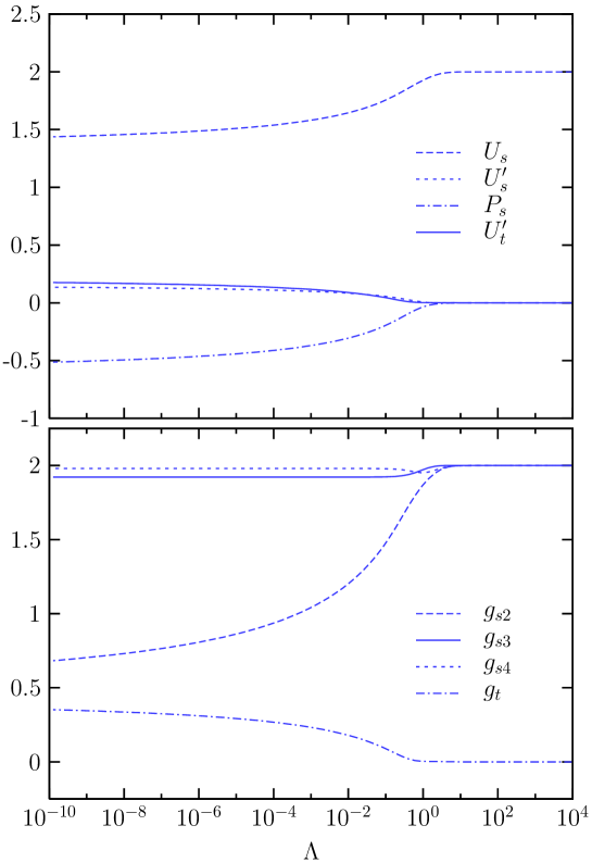
Figure 1: (Color online) Vertex flow for the Hubbard model at quarter-filling ($n=1/2$) and $U=1$; upper panel: flow of the renormalized real space interactions, lower panel: flow of the momentum space couplings.

In Fig. 1 we show results for the renormalized real space interactions together with the corresponding momentum space couplings, as obtained by integrating the flow equations for the Hubbard model at quarter-filling and $T=0$. Note that the couplings converge to finite fixed-point values in the limit $\Lambda\to 0$, but the convergence is very slow, except for the momentum space couplings $g^{\Lambda}_{s3}$ and $g^{\Lambda}_{s4}$. This can be traced back to the familiar behavior of the so-called backscattering coupling $g^{\Lambda}_{1\perp}=\frac{1}{2}\,(g^{\Lambda}_{s2}-g^{\Lambda}_{t})$, that is the amplitude for the exchange of two particles with opposite spin at opposite Fermi points. Backscattering is known to vanish logarithmically in the low-energy limit for spin-rotation invariant spin-$\frac{1}{2}$ Luttinger liquids.Voi We emphasize that this logarithmic behavior is not promoted to a power law by higher order terms beyond our approximation. By contrast, the linear combination of couplings which determines the Luttinger-liquid parameter $K_{\rho}$ converges very quickly to a finite fixed-point value (see below).

Due to the above parametrization of the vertex by real space interactions which do not extend beyond nearest neighbors on the lattice, the self-energy generated by the flow equations is frequency independent and tridiagonal in real space. Inserting the spin and real space structure of $\Gamma^{\Lambda}$ into the general flow equation for the self-energy, Eq. (16) in Ref. AEX, , one obtains

$$\frac{\partial}{\partial\Lambda}\,\Sigma^{\Lambda}_{j,j} = -\frac{1}{4\pi}\sum_{\omega=\pm\Lambda}\Big{[}\,U_{s}^{\Lambda}\,\tilde{G}^{\Lambda}_{j,j}(i\omega)+({U^{\prime}_{s}}^{\Lambda}+3{U^{\prime}_{t}}^{\Lambda})\sum_{r=\pm 1}\,\tilde{G}^{\Lambda}_{j+r,j+r}(i\omega)\,\Big{]}$$

$$\frac{\partial}{\partial\Lambda}\,\Sigma^{\Lambda}_{j,j\pm 1} = -\frac{1}{4\pi}\sum_{\omega=\pm\Lambda}\left[\,({U^{\prime}_{s}}^{\Lambda}-3{U^{\prime}_{t}}^{\Lambda})\,\tilde{G}^{\Lambda}_{j,j\pm 1}(i\omega)+P^{\Lambda}_{s}\,\tilde{G}^{\Lambda}_{j\pm 1,j}(i\omega)\,\right]\;,$$ (19)

where $\tilde{G}^{\Lambda}=(G_{0}^{-1}-\Sigma^{\Lambda})^{-1}$. These equations can be solved very efficiently,Ens so that very large systems with up to $10^{7}$ sites can be treated.

At $T>0$ the Matsubara frequencies are discrete, and a sharp frequency cutoff therefore leads to discontinuities in the flow. To avoid ambiguities and numerical problems associated with these discontinuities one may choose a smooth frequency cutoff as in Ref. EMX, . Alternatively, one can rewrite the Matsubara sum as a frequency integral with a suitable weight function, as described in detail in the Appendix. The latter procedure leads to a particularly simple and numerically convenient extension of the flow equations to finite temperatures. In the flow equations (18) and (II.2) one has to replace $\omega=\pm\Lambda$ by $\omega=\pm\omega_{n}^{\Lambda}$, where $\omega_{n}^{\Lambda}$ is the Matsubara frequency which is closest to $\Lambda$. The function $h_{\alpha^{\prime}\alpha^{\prime\prime}}^{\alpha}(\omega)$ remains the same. At $T>0$ the flow equations can be solved for systems with up to $10^{5}$ sites without extensive numerical effort.

When using a sharp cutoff with $\tilde{G}^{\Lambda}$ defined above it makes no difference whether the bare impurity potential is put into $G_{0}^{-1}$ or $\Sigma^{\Lambda}$; we choose to include it in the initial condition of $\Sigma^{\Lambda}$ at $\Lambda=\infty$. Due to the slow decay of $G$ at large frequencies, the integration of the flow equation for $\Sigma$ from $\Lambda=\infty$ to $\Lambda=\Lambda_{0}$ yields a contribution which remains finite even in the limit $\Lambda_{0}\to\infty$.AEX For the extended Hubbard model this contribution is given by $\Sigma^{\Lambda_{0}}_{j,j}=U/2+2U^{\prime}$ for $j=2,\dots,L\!-\!1$ and $\Sigma^{\Lambda_{0}}_{1,1}=\Sigma^{\Lambda_{0}}_{L,L}=U/2+U^{\prime}$. The numerical integration of the flow is started at a sufficiently large $\Lambda_{0}$ with $\Sigma^{\Lambda_{0}}$ as initial condition.

II.3 Calculation of ${\boldsymbol{K}_{\bf\rho}}$

The Luttinger-liquid parameter $K_{\rho}$ can be computed from the fixed-point couplings as obtained from the fRG. A relation between the fixed-point couplings and $K_{\rho}$ can be established via the exact solution of the fixed-point Hamiltonian of Luttinger liquids, the Luttinger model. Since the above simplified flow equations yield not only the correct low-energy asymptotics to second order in the renormalized interaction, but contain also all nonuniversal second order corrections at $\pm k_{F}$ at higher energy scales, the resulting $K_{\rho}$ is obtained correctly to second order in the interaction.

The Luttinger-liquid parameter $K_{\rho}$ is given by

$$K_{\rho}=\sqrt{\frac{1+(g_{\rho 4}-g_{\rho 2})/(\pi v_{F})}{1+(g_{\rho 4}+g_{\rho 2})/(\pi v_{F})}}\;.$$ (20)

The coupling constants $g_{\rho 2}$ and $g_{\rho 4}$ parametrize forward scattering interactions in the charge channel (which is spin symmetrized) between opposite and equal Fermi points, respectively. They are related to the bare singlet and triplet vertices of the Luttinger model by

$$g_{\rho 2} = \frac{1}{4}\,\big{(}\,\gamma_{s|\,k_{F},-k_{F};k_{F},-k_{F}}+3\gamma_{t|\,k_{F},-k_{F};k_{F},-k_{F}}\,\big{)}$$

$$g_{\rho 4} = \frac{1}{4}\,\gamma_{s|\,k_{F},k_{F};k_{F},k_{F}}\;.$$ (21)

These bare vertices are identical to the dynamical forward scattering limits of the full vertex $\Gamma$. On the other hand, the vertex $\Gamma^{\Lambda}$ obtained from the fRG with a frequency cutoff yields the static forward scattering limit for $\Lambda\to 0$.AEX For the Luttinger model, the static forward scattering limit of the vertex can be computed from the effective interactions $D_{\rho 2}(q,i\nu)$ and $D_{\rho 4}(q,i\nu)$, which are defined as the sum over all particle-hole chains with the bare interactions $g_{\rho 2}$ and $g_{\rho 4}$.Sol The summation becomes a simple geometric series if one introduces symmetric and antisymmetric combinations $g_{\rho\pm}=g_{\rho 4}\pm g_{\rho 2}$ and $D_{\rho\pm}(q,i\nu)=D_{\rho 4}(q,i\nu)\pm D_{\rho 2}(q,i\nu)$. The static limit of the effective interaction $D_{\rho\pm}(q,i\nu)$ yields the relation

$$g^{*}_{\rho\pm}=\frac{g_{\rho\pm}}{1-g_{\rho\pm}/(\pi v_{F})}$$ (22)

between the Luttinger-model couplings $g_{\rho\pm}$ and the fixed-point couplings

$$g^{*}_{\rho\pm}=\frac{1}{4}\,\big{[}\,g^{*}_{s4}\pm\big{(}\,g^{*}_{s2}+3g^{*}_{t}\,\big{)}\big{]}$$ (23)

from the fRG with frequency cutoff. Inverting (22) one obtains

$$K_{\rho}=\sqrt{\frac{1-g^{*}_{\rho+}/(\pi v_{F})}{1-g^{*}_{\rho-}/(\pi v_{F})}}\;.$$ (24)

The Fermi velocity $v_{F}$ can be computed from the self-energy for the translation invariant pure system as in the spinless case, AEX using the momentum representation of the flow equations (II.2).

The results for $K_{\rho}$ from the above procedure are correct to second order in the bare interaction for the Hubbard model and also for the extended Hubbard model. While the flowing couplings $g^{\Lambda}_{s2}$ and $g^{\Lambda}_{t}$ converge only logarithmically to their fixed-point values for $\Lambda\to 0$, the linear combination $g^{\Lambda}_{s2}+3g^{\Lambda}_{t}$ which enters $K_{\rho}$ converges much faster.

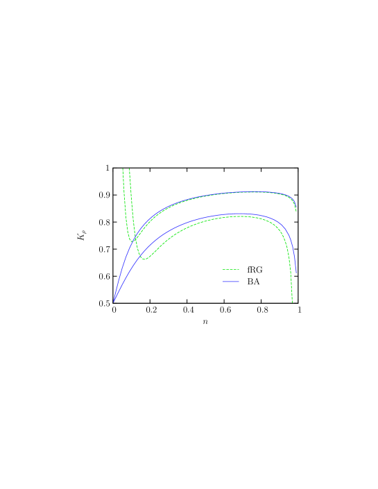
Figure 2: (Color online) Luttinger-liquid parameter $K_{\rho}$ for the Hubbard model as a function of electron density. Results from the fRG are compared to exact results from the Bethe ansatz. The upper curves are for $U=1$ and the lower ones for $U=2$.

In Fig. 2 we show results for $K_{\rho}$ for the Hubbard model as obtained from the fRG and, for comparison, from the exact Bethe ansatz solution.Sch The truncated fRG yields accurate results at weak coupling except for low densities and close to half-filling. In the latter case this failure is expected since umklapp scattering interactions renormalize toward strong coupling, even if the bare coupling is weak. At low densities already the bare dimensionless coupling $U/v_{F}$ is large for fixed finite $U$, simply because $v_{F}$ is proportional to $n$ for small $n$, such that neglected higher order terms become important. Note, for comparison, that for spinless fermions with a fixed nearest-neighbor interaction the bare dimensionless coupling at the Fermi level vanishes in the low-density limit.

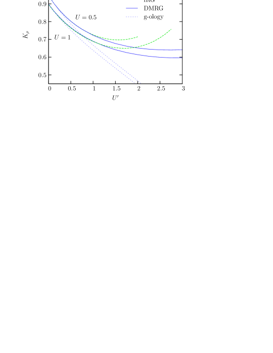
Figure 3: (Color online) Luttinger-liquid parameter $K_{\rho}$ for the quarter-filled extended Hubbard model as a function of $U^{\prime}$ for $U=0.5$ and $U=1$. Results from the fRG are compared to DMRG data and to results from a one-loop g-ology calculation.

For the extended Hubbard model Fig. 3 shows a comparison of fRG results for $K_{\rho}$ to DMRG data.EGN The fRG results are exact to second order in the interaction and are thus very accurate for weak $U$ and $U^{\prime}$. Results from a standard one-loop g-ology calculation Sol deviate quite strongly already for $U^{\prime}>0.5$. In the g-ology approach interaction processes are classified into backward scattering $(g_{1\perp})$, forward scattering involving electrons from opposite Fermi points $(g_{2\perp})$, from the same Fermi points $(g_{4\perp})$, and umklapp scattering $(g_{3\perp})$. All further momentum dependences of the vertex are discarded. This is justified by the irrelevance of these momentum dependences in the low-energy limit, but leads to deviations from the exact flow at finite scales, and therefore to less accurate results for the fixed-point couplings.

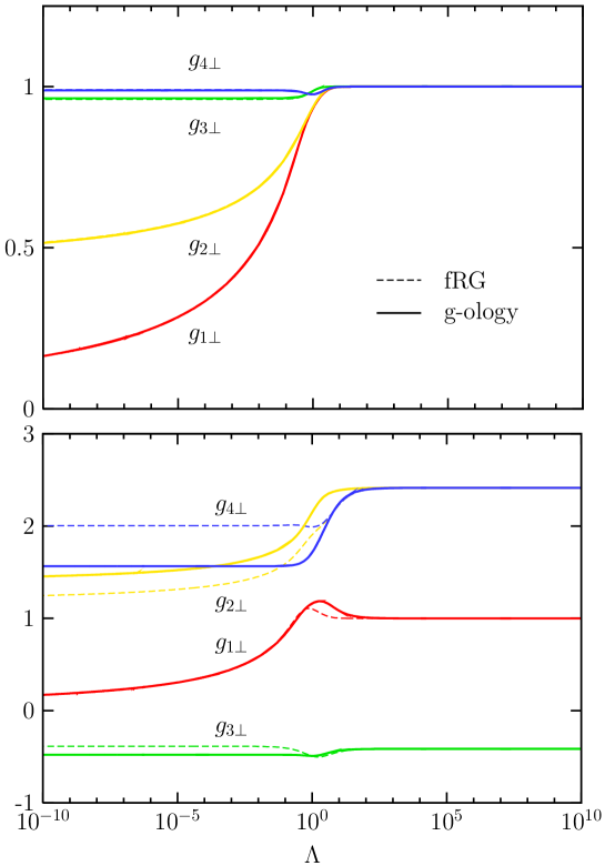
Figure 4: (Color online) Flow of the vertex on the Fermi points (in g-ology notation) at quarter-filling and $U=1$; upper panel: Hubbard model, lower panel: extended Hubbard model with $U^{\prime}=U/\sqrt{2}$. The fRG flow is compared to the one-loop g-ology flow; note that in the upper panel fRG and g-ology results almost coincide.

The flow of $g_{i\perp}^{\Lambda}$, $i=1,...,4$, is plotted in Fig. 4, in the upper panel for the quarter-filled Hubbard model with bare interaction $U=1$, and for the extended Hubbard model with $U^{\prime}=U/\sqrt{2}$ in the lower. The fRG result is compared to the result from a one-loop g-ology calculation. The backscattering coupling $g_{1\perp}$ vanishes logarithmically in both cases, as expected for the Luttinger-liquid fixed point.Voi For the pure Hubbard model the good agreement with g-ology results stems from the purely local interaction in real space, since in that case pronounced momentum dependences of the vertex develop only in the low-energy regime where the g-ology parametrization is a good approximation. By contrast, for the extended Hubbard model momentum dependences of the vertex which are not captured by the g-ology classification (except for small $\Lambda$) are obviously more important. A generalization of the g-ology parametrization of the vertex to higher dimensions, which amounts to neglecting the momentum dependence normal to the Fermi surface, is frequently used in one-loop fRG calculations in two dimensions.2dHubb The above comparison indicates that this parametrization works well for the pure Hubbard model, but could be improved for models with nonlocal interactions. The parametrization of the vertex by an effective short-range interaction used here could be easily extended to higher dimensions, where it will probably yield more accurate results, too. The relevance of an improved parametrization of the vertex beyond the conventional g-ology classification has also been demonstrated in a recent fRG analysis of the phase-diagram of the half-filled extended Hubbard model.TTC

III Results for observables

In this section we present and discuss explicit results for the spectral properties of single-particle excitations, the density profile, and the conductance for the Hubbard and extended Hubbard model with a single impurity, as obtained from the solution of the fRG flow equations. We also analyze excitations and density oscillations near a boundary, which corresponds to an infinite site impurity or a vanishing weak link. A comparison with DMRG results is made for the spectral weight at the Fermi level and for the density profile. For details on the computation of the relevant observables from the solution of the flow equations we refer to Ref. AEX, ; EMX, .

III.1 Single-particle excitations

Integrating the flow equation for the self-energy $\Sigma^{\Lambda}$ down to $\Lambda=0$ yields the physical self-energy $\Sigma$ and the single-particle propagator $G=(G_{0}^{-1}-\Sigma)^{-1}$. From the Green function $G$ the properties of single-particle excitations can be extracted. We focus on the local spectral function given by

$$\rho_{j}(\omega)=-\frac{1}{\pi}\,{\rm Im}\,G_{jj}(\omega+i0^{+})\;.$$ (25)

For a finite system this function is a finite sum of $\delta$-peaks of weight $w_{\lambda j}$, where $\lambda$ labels the eigenvalues of the effective single-particle Hamiltonian defined by $G$. Dividing the spectral weight $w_{\lambda j}$ by the level spacing yields the local density of states $D_{j}(\omega)$. Even-odd effects due to finite-size details in the spectral weight are averaged out by averaging over neighboring eigenvalues.

For $\omega\to 0$ the spectral weights and the local density of states near a boundary or impurity are ultimately suppressed according to a power law with the boundary exponent

$$\alpha_{B}=\frac{1}{2K_{\rho}}+\frac{1}{2K_{\sigma}}-1$$ (26)

with $K_{\sigma}=1$ for spin-rotation invariant systems. Gia However, due to the slow logarithmic decrease of the two-particle backscattering amplitude, the fixed-point value of $K_{\sigma}$ is reached only logarithmically from above. Hence, we can expect that the asymptotic value of $\alpha_{B}$ is usually reached only very slowly from below.

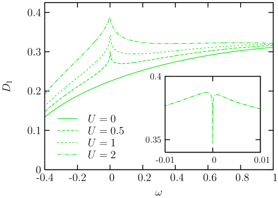
Figure 5: (Color online) Local density of states at the boundary of a Hubbard chain of length $L=4096$ at quarter-filling and various interaction strengths $U$; the inset shows results for $U=2$ and $L=10^{6}$ at very low $\omega$.

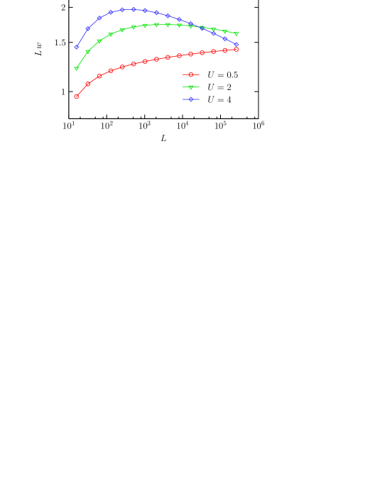
Figure 6: (Color online) Spectral weight at the Fermi level at the boundary of a quarter-filled Hubbard chain as a function of system size $L$, for various different interaction strengths.

The local density of states at the boundary of a quarter-filled Hubbard chain, computed by the fRG, is shown in Fig. 5 for various values of the local interaction $U$. Contrary to the expected asymptotic power-law suppression, the spectral weight near the chemical potential is strongly enhanced. The predicted suppression occurs only at very small energies for sufficiently large systems. In the main panel of Fig. 5 the crossover to the asymptotic behavior cannot be observed, as the finite size cutoff $\sim\pi v_{F}/L$ is too large. Results for a larger system with $L=10^{6}$ sites at $U=2$ in the inset show the crossover to the asymptotic suppression, albeit only at very small energies. The dependence of the boundary spectral weight at the Fermi level on the system size $L$ is plotted in Fig. 6. The $L$-dependence of the spectral weight at zero energy is expected to display the same asymptotic power-law behavior for large $L$ as the $\omega$-dependence discussed above. Instead of decreasing with increasing $L$, the spectral weight increases even for rather large systems for small and moderate values of $U$. For $U>2$ the crossover to a suppression is visible in Fig. 6. For $U=0.5$ only an increase is obtained up to the largest systems studied. The crossover scale depends sensitively on the interaction strength $U$; for small $U$ it is exponentially large in $v_{F}/U$.

The above behavior of the spectral weight and density of states near a boundary of the Hubbard chain, that is a pronounced increase preceding the asymptotic power-law suppression, is captured qualitatively even by the Hartree-Fock approximation.SMX ; MMX This is at first sight surprising, as the Hartree-Fock theory does not capture any Luttinger-liquid features in the bulk of a translation invariant system. The initial increase of $D_{j}(\omega)$ near a boundary is actually obtained already within perturbation theory at first order in the interaction,MMX

$$D_{j}(\omega)=D_{j}^{0}(\omega)\,\left[\,1+\frac{\tilde{V}(0)-z\tilde{V}(2k_{F})}{2\pi v_{F}}\,\ln|\omega/\epsilon_{F}|+{\cal O}(\tilde{V}^{2})\,\right]\;,$$ (27)

where $D_{j}^{0}(\omega)$ is the noninteracting density of states, $\tilde{V}(q)$ the Fourier transform of the real space interaction, and $z$ the number of spin components. For spinless fermions ($z=1$) with repulsive interactions the coefficient in front of the logarithm is always positive such that the first order term leads to a suppression of $D_{j}(\omega)$. For the Hubbard model, one has $z=2$ and $\tilde{V}(0)-2\tilde{V}(2k_{F})=-U$ is negative for repulsive $U$. Hence, at least for weak $U$ the density of states increases for decreasing $\omega$ until terms beyond first order become important. For the extended Hubbard model, $\tilde{V}(0)-2\tilde{V}(2k_{F})=2U^{\prime}[1-2\cos(2k_{F})]-U$, which can be positive or negative for $U,U^{\prime}>0$, depending on the density and the relative strength of the two interaction parameters. At quarter-filling $\tilde{V}(0)-2\tilde{V}(2k_{F})$ is negative and therefore leads to an enhanced density of states for $U^{\prime}<U/2$.

Using g-ology notation, one can write $\tilde{V}(0)-2\tilde{V}(2k_{F})=g_{2\perp}-2g_{1\perp}$, which reveals that substantial two-particle backscattering ($g_{1\perp}>g_{2\perp}/2$) is necessary to obtain an enhancement of $D_{j}(\omega)$ for repulsive interactions. Backscattering vanishes at the Luttinger-liquid fixed point, but only very slowly. In case of a negative $\tilde{V}(0)-2\tilde{V}(2k_{F})$ the crossover to a suppression of $D_{j}(\omega)$ is due to higher order terms, which are expected to become important when the first order correction is of order one, that is for energies below the scale

$$\omega_{c}=\epsilon_{F}\exp\left(\frac{2\pi v_{F}}{\tilde{V}(0)-2\tilde{V}(2k_{F})}\right)\;,$$ (28)

corresponding to a system size $L_{c}=\pi v_{F}/\omega_{c}$. The scale $\omega_{c}$ is exponentially small for weak interactions. A more accurate analytical estimate of the crossover scale from enhancement to suppression has been derived for the Hubbard model within Hartree-Fock approximation in Ref. MMX, . In a renormalization group treatment $\omega_{c}$ is somewhat enhanced by the downward renormalization of backscattering.

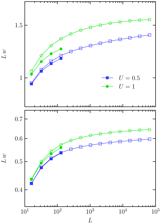
Figure 7: (Color online) Spectral weight at the Fermi level near a boundary (upper panel) and a hopping impurity $t^{\prime}=0.5$ (lower panel) as a function of system size $L$ for the Hubbard model at quarter-filling and different interaction strengths $U$; results from the fRG (open symbols) are compared to DMRG data (filled symbols).

A comparison of fRG results with DMRG data dmrgspec for the spectral weight at the Fermi level is shown in Fig. 7, for a boundary site in the upper panel, and near a hopping impurity of strength $t^{\prime}=0.5$ in the lower. The agreement improves at weaker coupling, as expected, and is generally better for the impurity case, compared to the boundary case. The larger errors in the boundary case are probably due to our approximate translation invariant parametrization of the two-particle vertex. Boundaries and to a minor extent impurities spoil the translation invariance of the two-particle vertex. Although the deviations from translation invariance of the vertex become irrelevant in the low-energy or long-distance limit, and therefore do not affect the asymptotic behavior, they are nevertheless present at intermediate scales. This feedback of impurities into the vertex increases of course with the impurity strength and is thus particularly important near a boundary. The scale for the crossover from enhancement to suppression of spectral weight discussed above depends sensitively on effective interactions at intermediate scales and can therefore be shifted considerably even by relatively small errors in that regime.

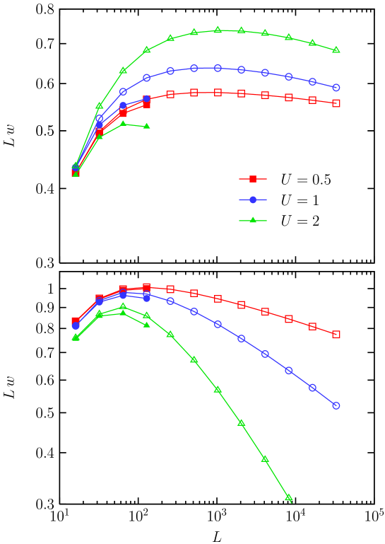
Figure 8: (Color online) Spectral weight at the Fermi level near a hopping impurity $t^{\prime}=0.5$ as a function of system size $L$ for the extended Hubbard model with $U^{\prime}=U/\sqrt{2}$, for various choices of $U$; upper panel: $n=1/2$ (leading to sizable backscattering), lower panel: $n=3/4$ (leading to small backscattering); results from the fRG (open symbols) are compared to DMRG data (filled symbols).

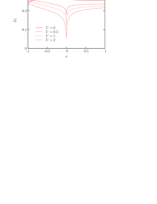
Figure 9: (Color online) Local density of states near a hopping impurity $t^{\prime}=0.5$ in an extended Hubbard model with density $n=3/4$ and interaction $U^{\prime}=U/\sqrt{2}$ (leading to a small backscattering interaction) for various choices of $U$. The size of the chain is $L=4096$.

With the additional nearest-neighbor interaction in the extended Hubbard model it is possible to tune parameters such that the two-particle backscattering amplitude becomes negligible. In that case the asymptotic power-law suppression of spectral weight should be free from logarithmic corrections and accessible already for smaller systems and at higher energy scales. The bare backscattering interaction in the extended Hubbard model is given by $g_{1\perp}=U+2U^{\prime}\cos(2k_{F})$ and therefore vanishes for $U^{\prime}=-U/[2\cos(2k_{F})]$, which is repulsive for $U>0$ if $n>1/2$. In a one-loop calculation a slightly different value of $U^{\prime}$ has to be chosen to obtain a negligible renormalized $g_{1\perp}^{\Lambda}$ for small finite $\Lambda$, since the flow generates backscattering terms at intermediate scales even if the bare $g_{1\perp}$ vanishes. In Fig. 8 we show fRG and DMRG results dmrgspec for the spectral weight of the extended Hubbard model at the Fermi level near a hopping impurity. In the upper panel a generic case with sizable backscattering is shown, while the parameters leading to the curves in the lower panel have been chosen such that the two-particle backscattering amplitude is negligible at low energy. Only in the latter case a pronounced suppression of spectral weight is reached already for intermediate system size, similar to the behavior obtained previously for spinless fermions with nearest-neighbor interaction.MMSS ; AEX This is also reflected in the energy dependence of the local density of states near the impurity. For parameters leading to negligible two-particle backscattering as in Fig. 9 the suppression of the density of states sets in already at relatively high energies and is not preceded by any interaction-induced increase. Note also that the fRG results are much more accurate for small backscattering, as can be seen by comparing the agreement with DMRG data in the upper and lower panel of Fig. 8 especially for larger $U$. This indicates that the influence of the impurity on the vertex flow, which we have neglected, is more important in the presence of a sizable backscattering interaction.

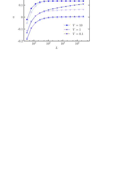
Figure 10: (Color online) Logarithmic derivative of the spectral weight at the Fermi level on the site next to a site impurity of strength $V$ in the center of the chain as a function of system size $L$, for the extended Hubbard model with interaction parameters $U=1$, $U^{\prime}=0.65$, and density $n=3/4$; here the filled symbols are fRG, the open symbols Hartree-Fock results.

In the case of a negligible backscattering amplitude, the spectral weight at the Fermi level approaches a power law without logarithmic corrections for accessible system sizes if the impurity is sufficiently strong. The power law is seen most clearly by plotting the effective exponent $\alpha(L)$, that is the negative logarithmic derivative of the spectral weight with respect to the system size. Fig. 10 shows $\alpha(L)$ on the site next to a site impurity of strength $V$ for the extended Hubbard model with $U=1$, $U^{\prime}=0.65$, and $n=3/4$. The backscattering amplitude is very small for these parameters. The fRG results approach the expected universal $V$-independent power law for large $L$, but only very slowly for small $V$. For a weak bare impurity potential $V$, the crossover to a strong effective impurity occurs only on a large length scale of order $V^{2/(K_{\rho}-1)}\,$.KF For $V=0.1$ this scale is obviously well above the largest system size reached in Fig. 10. The Hartree-Fock approximation also yields power laws for large $L$, but the exponents depend on the impurity parameters. This failure of Hartree-Fock theory was already observed earlier for spinless fermions.MMSS

The effective exponent obtained from the fRG calculation agrees with the exact boundary exponent to linear order in the bare interaction, but not to quadratic order. To improve this, the frequency dependence of the two-particle vertex, which generates a frequency dependence of the self-energy, has to be taken into account. This is also necessary to describe inelastic processes and to capture the anomalous dimension of the bulk system. These effects could be included in an improved scheme by inserting the second order vertex into the flow equation for the self-energy without neglecting its frequency dependence.

III.2 Density profile

Boundaries and impurities induce a density profile with long-range Friedel oscillations, which are expected to decay as a power law with exponent $(K_{\rho}+K_{\sigma})/2$ at long distances, where $K_{\sigma}=1$ for spin-rotation invariant systems.EG For weak impurities linear response theory predicts a decay as $|j-j_{0}|^{1-K_{\rho}-K_{\sigma}}$ at intermediate distances.

The density profile has to be computed from an additional flow equation, since the local density is a composite operator whose renormalization is not well described by the propagator obtained from the truncated flow of $\Sigma^{\Lambda}$. The flow equation for $n_{j}^{\Lambda}$ can be derived by computing the shift of the grand canonical potential $\Omega^{\Lambda}$ generated by a small field $\phi_{j}$ coupled to the local density. Its general structure at $T=0$ is described in Ref. AEX, . From Eqs. (38) and (40) in that article one can easily obtain the concrete flow equation for the case of the extended Hubbard model.

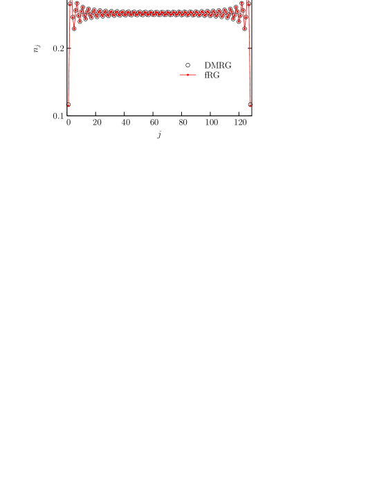
Figure 11: (Color online) Density profile $n_{j}$ for the Hubbard model with $128$ sites and interaction strength $U=1$ at quarter-filling; fRG results are compared to DMRG data.

As an additional benchmark for the fRG technique, we compare in Fig. 11 fRG and DMRG results for the density profile $n_{j}$ for a quarter-filled Hubbard chain with $L=128$ lattice sites and open boundaries. Friedel oscillations emerge from both boundaries and interfere in the center of the chain. The fRG results have been shifted by a small constant amount to allow for a better comparison of the oscillations. Note that the mean value of $n_{j}$ in the tails of the oscillations deviates from the average density by a finite size correction of order $1/L$, which is related to the asymmetry of the oscillations near the boundaries.

The long-distance behavior of the density oscillations as obtained within the fRG scheme has been analyzed in detail for spinless fermions in Ref. AEX, . For fermions with spin, asymptotic power laws can be identified only for special parameters leading to negligible two-particle backscattering. In general, the asymptotic behavior of Friedel oscillations is realized only at very long distances, and the power laws are modified by logarithmic corrections.

III.3 Conductance

For the computation of the conductance a finite interacting chain is connected to two semi-infinite noninteracting leads, with a smooth decay of the interaction at the contacts. The presence of leads modifies the propagator in the interacting region only via the boundary potential $V^{\rm lead}$, Eq. (2). In linear response the conductance is given by EMX ; Oguri

$$G(T)=-\frac{2e^{2}}{h}\int_{-2-\mu_{0}}^{2-\mu_{0}}|t(\varepsilon,T)|^{2}\;f^{\prime}(\varepsilon)\;d\varepsilon$$ (29)

with $|t(\varepsilon,T)|^{2}=[4-(\mu_{0}+\varepsilon)^{2}]\,|G_{1,L}(\varepsilon,T)|^{2}$, and $f$ the Fermi function. The factor two is due to the spin degeneracy. Within our approximation scheme, $\Sigma^{\Lambda}$ has no imaginary part, which implies that there are no vertex corrections, such that the conductance is fully determined by boundary matrix element of the single-particle propagator $G_{1,L}(\varepsilon,T)$. Oguri

For a system of spinless fermions with a single impurity it was already shown that the conductance obtained from the truncated fRG obeys the expected power laws, in particular $G(T)\propto T^{2\alpha_{B}}$ at low $T$, and one-parameter scaling behavior. EMX ; MAX The corresponding scaling function agrees remarkably well with an exact result for $K_{\rho}=1/2$, although the interaction required to obtain such a small $K_{\rho}$ is quite strong. The more complex temperature dependence of the conductance in the case of a double barrier at or near a resonance is also fully captured by the fRG.EMX ; MEX

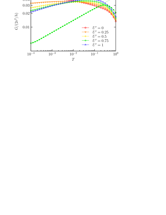
Figure 12: (Color online) Temperature dependence of the conductance for the extended Hubbard model with $L=10^{4}$ sites and a single site impurity of strength $V=10$, for a Hubbard interaction $U=1$ and various choices of $U^{\prime}$; the density is $n=1/2$, except for the lowest curve, which has been obtained for $n=3/4$ and $U^{\prime}=0.65$ (leading to a very small backscattering interaction); the dashed line is a power-law fit for the latter parameter set.

Fig. 12 shows typical fRG results for the temperature dependence of the conductance for the extended Hubbard model with a single strong site impurity ($V=10$). Similar results were obtained for a hopping impurity. The considered size $L=10^{4}$ corresponds to interacting wires in the micrometer range, which is the typical size of quantum wires available for transport experiments. For $U^{\prime}=0$ the conductance increases as a function of decreasing $T$ down to the lowest temperatures in the plot. For increasing nearest-neighbor interactions $U^{\prime}$ a suppression of $G(T)$ at low $T$ becomes visible, but in all the data obtained at quarter-filling the suppression is much less pronounced than what one expects from the asymptotic power law with exponent $2\alpha_{B}$. By contrast, the suppression is much stronger and follows the expected power law more closely if parameters are chosen such that two-particle backscattering becomes negligible at low $T$, as can be seen from the conductance curve for $n=3/4$ and $U^{\prime}=0.65$ in Fig. 12. The value of $K_{\rho}$ for these parameters almost coincides with the one for another parameter set in the plot, $n=1/2$ and $U^{\prime}=0.75$, but the behavior of $G(T)$ is completely different. Note that at $T\sim\pi v_{F}/L$ finite size effects set in, as can be seen at the low $T$ end of some of the curves in the figure. An enhancement of the conductance due to backscattering has been found already earlier in a renormalization group study of impurity scattering in the g-ology model.YGM

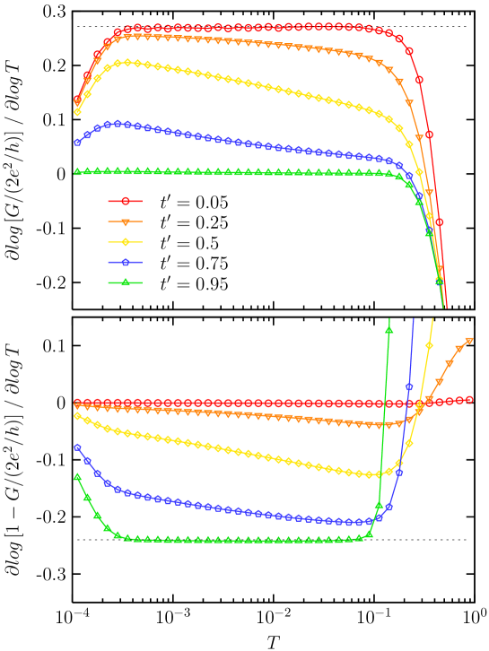
Figure 13: (Color online) Logarithmic temperature derivative of the conductance (upper panel) and of its deviation from the unitarity limit (lower panel) for the extended Hubbard model with $L=10^{4}$ sites and various hopping impurities. The density is $n=3/4$, interaction parameters are $U=1$ and $U^{\prime}=0.65$. The dashed horizontal lines highlight power-law behavior.

Results for the conductance of the extended Hubbard model with a hopping impurity with various amplitudes $t^{\prime}$ are shown in Fig. 13. The bulk parameters have been chosen such that the two-particle backscattering is practically zero at low $T$. From the plot of the logarithmic derivative of $G(T)$ in the upper panel one can see that for a strong impurity (small $t^{\prime}$) the conductance follows a well defined power law $G(T)\propto T^{2\alpha_{B}}$ over a large temperature range. For intermediate $t^{\prime}$ the curves approach the asymptotic exponent at low $T$ from below, but do not reach it before finite size effects lead to a saturation of $G(T)$ for $T<\pi v_{F}/L$. For the weakest impurity in the plot, $t^{\prime}=0.95$, the conductance remains very close to the unitarity limit. However, the plot of the logarithmic derivative of $1-G/(2e^{2}/h)$ in the lower panel of Fig. 13 shows that $1-G/(2e^{2}/h)$ increases as $T^{K_{\rho}-1}$ for decreasing $T$, as expected for a weak impurity in the perturbative regime.KF The effective exponents indicated by the two horizontal lines in the figure deviate from the exact values (determined from the DMRG result EGN for $K_{\rho}$) by about $20\,\%$ in the case of $2\alpha_{B}$ and only by $5\,\%$ for $K_{\rho}-1$. Results for the conductance of a wire with a double-barrier impurity at or near resonance will be presented in a forthcoming publication.AEM

IV Conclusion

We have derived a fRG-based computation scheme for the one-dimensional extended Hubbard model with a single static impurity, extending previous work for spinless fermions AEX ; EMX to spin-$\frac{1}{2}$ fermions. The underlying approximations are devised for weak short-range interactions and arbitrary impurity potentials. Various observables have been computed: the local density of states near boundaries and impurities, the density profile, and the temperature dependence of the linear conductance. Results have been checked against DMRG data, for those observables and system sizes for which such data could be obtained. The general agreement is good at weak coupling, but for intermediate interaction strengths with sizable two-particle backscattering and strong impurities the deviations are significantly larger than for spinless fermions. We suspect that the neglected influence of impurities on vertex renormalization at high energy and short length scales is more important for fermions with spin.

Two-particle backscattering of particles with opposite spin at opposite Fermi points leads to two important effects, not present in the case of spinless fermions. First, the expected decrease of spectral weight and of the conductance at low energy scales is often preceded by an increase, which can be particularly pronounced for the density of states near an impurity or boundary as a function of $\omega$. For the density of states near a boundary this effect has been found already earlier within a Hartree-Fock and DMRG study of the Hubbard model,SMX ; MMX and for the conductance by a renormalization group analysis of the g-ology model.YGM Second, the asymptotic low-energy power laws are usually modified by logarithmic corrections. In the extended Hubbard model the backscattering can be eliminated for a special fine-tuned choice of parameters. Then the results are very similar to those for spinless fermions. For weak and intermediate impurity strengths the asymptotic low-energy behavior is approached only at rather low scales, which are accessible only for very large systems. This slow convergence was observed already for spinless fermions MMSS ; AEX ; EMX and holds also in the absence of two-particle backscattering.

For systems with long-range interactions backscattering is strongly reduced compared to forward scattering. This seems to be the case in carbon nanotubes.cnt Hence, the conductance can be expected to follow the asymptotic power law at accessible temperature scales for sufficiently strong impurities in these systems, as is indicated also by experiments.Yao However, the effects due to two-particle backscattering should be observable in systems with a screened Coulomb interaction.

Acknowledgments:
We thank Manfred Salmhofer for valuable discussions, Satoshi Nishimoto for providing the DMRG data of $K_{\rho}$ in the extended Hubbard model, and Roland Gersch for a critical reading of the manuscript. V.M. and K.S. are grateful to the Deutsche Forschungsgemeinschaft (SFB 602) for financial support.

Appendix A Frequency cutoff at finite temperature

In this appendix we derive a convenient implementation of a sharp frequency cutoff at finite temperature. The idea is roughly to rewrite the Matsubara sum as an integral over a piecewise constant function and then to introduce a sharp cutoff on this continuous frequency as usual.

In the 1PI scheme SH the flow equation with frequency cutoff at zero temperature has the form (assuming no frequency shift along the loop)Ens

$$\frac{\partial\Upsilon^{\Lambda}}{\partial\Lambda}=\int\frac{d\omega}{2\pi}\;\delta_{\epsilon}(|\omega|-\Lambda)\;f\bigl{(}\Theta_{\epsilon}(|\omega|-\Lambda),\omega,\Upsilon^{\Lambda}\bigr{)}\;.$$ (30)

Here $\Upsilon^{\Lambda}$ is the generating functional for the 1PI vertex functions, and $f(t,\omega,\Upsilon^{\Lambda})$ represents the right-hand side of the flow equations including the momentum integral, but with the integral over the Matsubara frequency $\omega$ written explicitly. $\Theta_{\epsilon}(x)$ is a step function smoothed on a scale $\epsilon$, and $\delta_{\epsilon}(x)=\partial_{x}\Theta_{\epsilon}(x)$. The $\omega$ integral gives finite contributions near $|\omega|=\Lambda$, hence $\Upsilon^{\Lambda}$ is a continuous function of $\Lambda$. Then the limit $\epsilon\to 0$ can be performed using Morris’ lemma,Mor

$$\frac{\partial\Upsilon^{\Lambda}}{\partial\Lambda}\overset{\epsilon\to 0}{\longrightarrow}\int\frac{d\omega}{2\pi}\;\delta(|\omega|-\Lambda)\int_{0}^{1}dt\;f\bigl{(}t,\omega,\Upsilon^{\Lambda}\bigr{)}=\frac{1}{2\pi}\sum_{\omega=\pm\Lambda}\int_{0}^{1}dt\;f\bigl{(}t,\omega,\Upsilon^{\Lambda}\bigr{)}.$$ (31)

The right-hand side is independent of the explicit cutoff function $\Theta_{\epsilon}(x)$, therefore the vertex functions in $\Upsilon^{\Lambda}$ are smooth not only in $\Lambda$ but also as functions of all external frequencies.

In our previous work at finite temperatureEMX the flow equation (30) with discrete Matsubara frequencies reads

$$\frac{\partial\Upsilon^{\Lambda}}{\partial\Lambda} =T\sum_{n}\delta_{\epsilon}(|\omega_{n}|-\Lambda)\;f\bigl{(}\Theta_{\epsilon}(|\omega_{n}|-\Lambda),\omega_{n},\Upsilon^{\Lambda}\bigr{)}.$$ (32)

In the limit $\epsilon\to 0$ the right-hand side contains a $\delta$ function and $\Upsilon^{\Lambda}$ jumps as $\Lambda$ passes $\omega_{n}$, hence the Morris lemma which requires continuity of $\Upsilon^{\Lambda}$ cannot be applied. We have therefore used a smooth cutoff, which renders the numerics relatively slow. Instead, we now propose a new sharp cutoff which allows to apply the Morris lemma. This reduces the runtime significantly and enables us to access another order of magnitude in system size and temperature.

First, we rewrite the Matsubara sum as an integral over a continuous frequency $\omega$ with a weight function peaked in non-overlapping neighborhoods of width $\eta$ around each $\omega_{n}$,

$$T\sum_{n}f(\omega_{n})=\int d\omega\;T\sum_{n}\delta_{\eta}(\omega-\omega_{n})\;f(M(\omega))$$ (33)

where $\int d\omega\,\delta_{\eta}(\omega-\omega_{n})=1$ and $M(\omega)$ returns the discrete Matsubara frequency $\omega_{n}$ closest to $\omega$. Hence, $f$ is a piecewise constant function of a continuous variable $\omega$. At this stage, the cutoff function in $\omega$ is introduced in the bare action. This leads to the flow equation

$$\frac{\partial\Upsilon^{\Lambda}}{\partial\Lambda} =\int d\omega\;T\sum_{n}\delta_{\eta}(\omega-\omega_{n})\;\delta_{\epsilon}(|\omega|-\Lambda)\;f\bigl{(}\Theta_{\epsilon}(|\omega|-\Lambda),M(\omega),\Upsilon^{\Lambda}\bigr{)}.$$ (34)

If we take the limit $\eta\to 0$ first we again obtain equation (32), which is the smooth cutoff limit. For finite $\eta$, however, Morris’ lemma gives

$$\frac{\partial\Upsilon^{\Lambda}}{\partial\Lambda} \overset{\epsilon\to 0}{\longrightarrow}\int d\omega\;T\sum_{n}\delta_{\eta}(\omega-\omega_{n})\;\delta(|\omega|-\Lambda)\int_{0}^{1}dt\;f\bigl{(}t,M(\omega),\Upsilon^{\Lambda}\bigr{)}$$

$$=T\sum_{n}\delta_{\eta}(|\omega_{n}|-\Lambda)\int_{0}^{1}dt\;f\bigl{(}t,\omega_{n},\Upsilon^{\Lambda}\bigr{)}.$$ (35)

For each $\omega_{n}$ separately this is an autonomous differential equation, hence the result is independent of the shape of $\delta_{\eta}(x)$. A convenient choice is a box of height $1/(2\pi T)$ and width $2\pi T$ centered around the Matsubara frequency $\omega_{n}$, that is, $\delta_{\eta}(x)=1/(2\pi T)$ for $|x|<\pi T$ and $0$ otherwise, which leads to the final result

$$\frac{\partial\Upsilon^{\Lambda}}{\partial\Lambda} =\frac{1}{2\pi}\sum_{\omega_{n}\approx\pm\Lambda}\int_{0}^{1}dt\;f\bigl{(}t,\omega_{n},\Upsilon^{\Lambda}\bigr{)}.$$ (36)

Comparison with equation (31) shows that the only change necessary at finite temperature is to replace the loop frequency $\omega=\pm\Lambda$ on the right-hand side by the nearest discrete Matsubara frequency. We have checked numerically that indeed this new sharp cutoff gives the same results as the previous smooth cutoff for the conductance $G(T)$ curves in a dramatically reduced runtime.

References

- (1) T. Giamarchi, Quantum Physics in One Dimension (Oxford University Press, New York, 2004).
- (2) For a review on Luttinger liquids, see J. Voit, Rep. Prog. Phys. 58, 977 (1995).
- (3) A. Luther and I. Peschel, Phys. Rev. B 9, 2911 (1974).
- (4) D.C. Mattis, J. Math. Phys. 15, 609 (1974).
- (5) W. Apel and T.M. Rice, Phys. Rev. B 26, 7063 (1982).
- (6) T. Giamarchi and H.J. Schulz, Phys. Rev. B 37, 325 (1988).
- (7) C.L. Kane and M.P.A. Fisher, Phys. Rev. B 46, 15233 (1992); Phys. Rev. Lett. 68, 1220 (1992).
- (8) A. Furusaki and N. Nagaosa, Phys. Rev. B 47, 4631 (1993).
- (9) K.A. Matveev, D. Yue, and L.I. Glazman, Phys. Rev. Lett. 71, 3351 (1993); D. Yue, L.I. Glazman, and K.A. Matveev, Phys. Rev. B 49, 1966 (1994).
- (10) For a review on the experimental verification of Luttinger-liquid behavior, see K. Schönhammer, J. Phys.: Condens. Matter 14, 12783 (2002).
- (11) V. Meden, W. Metzner, U. Schollwöck, and K. Schönhammer, Phys. Rev. B 65, 045318 (2002); J. Low Temp. Phys. 126, 1147 (2002).
- (12) S. Andergassen, T. Enss, V. Meden, W. Metzner, U. Schollwöck, and K. Schönhammer, Phys. Rev. B 70, 075102 (2004).
- (13) T. Enss, V. Meden, S. Andergassen, X. Barnabé-Thériault, W. Metzner, and K. Schönhammer, Phys. Rev. B 71, 155401 (2005).
- (14) V. Meden, S. Andergassen, W. Metzner, U. Schollwöck, and K. Schönhammer, Europhys. Lett. 64, 769 (2003).
- (15) For a recent review on DMRG, see U. Schollwöck, Rev. Mod. Phys. 77, 259 (2005).
- (16) V. Meden, T. Enss, S. Andergassen, W. Metzner, and K. Schönhammer, Phys. Rev. B 71, 041302(R) (2005).
- (17) V. Meden and U. Schollwöck, Phys. Rev. B 67, 035106 (2003); ibid 193303 (2003).
- (18) X. Barnabé-Thériault, A. Sedeki, V. Meden, and K. Schönhammer, Phys. Rev. Lett. 94, 136405 (2005).
- (19) K. Schönhammer, V. Meden, W. Metzner, U. Schollwöck, and O. Gunnarsson, Phys. Rev. B 61, 4393 (2000).
- (20) V. Meden, W. Metzner, U. Schollwöck, O. Schneider, T. Stauber, and K. Schönhammer, Eur. Phys. J. B 16, 631 (2000).
- (21) E.H. Lieb and F.Y. Wu, Phys. Rev. Lett. 20, 1445 (1968).
- (22) H.J. Schulz, Phys. Rev. Lett. 64, 2831 (1990); H. Frahm and V.E. Korepin, Phys. Rev. B 42, 10553 (1990); N. Kawakami and S.K. Yang, Phys. Lett. A 148, 359 (1990).
- (23) C. Wetterich, Phys. Lett. B 301, 90 (1993).
- (24) T.R. Morris, Int. J. Mod. Phys. A 9, 2411 (1994).
- (25) For generic interacting Fermi systems, a concise derivation of the full hierarchy of flow equations for 1PI vertex functions is presented by M. Salmhofer and C. Honerkamp, Prog. Theor. Phys. 105, 1 (2001).
- (26) For a review, see J. Sólyom, Adv. Phys. 28, 201 (1979).
- (27) S. Andergassen, Ph.D. thesis, Universität Stuttgart 2006.
- (28) T. Enss, Ph.D. thesis, Universität Stuttgart 2005, URN: urn:nbn:de:bsz:93-opus-22587, URL: http://elib.uni-stuttgart.de/opus/volltexte/2005/2258/, cond-mat/0504703.
- (29) S. Ejima, F. Gebhard, and S. Nishimoto, Europhys. Lett. 70, 492 (2005); S. Nishimoto (private communication). For the Hubbard model, S. Ejima et al. showed that the difference between exact (Bethe ansatz) and DMRG results is below , for the extended Hubbard model the accuracy of the DMRG data is presumably of the same order.
- (30) D. Zanchi and H.J. Schulz, Phys. Rev. B 61, 13609 (2000); C.J. Halboth and W. Metzner, ibid 61, 7364 (2000); C. Honerkamp, M. Salmhofer, N. Furukawa, and T.M. Rice, ibid 63, 035109 (2001); A.P. Kampf and A.A. Katanin, ibid, 67, 125104 (2003).
- (31) K. Tam, S. Tsai, and D.K. Campbell, cond-mat/0505396.
- (32) The DMRG data for the local spectral weight at the Fermi level have been obtained by computing , where is the -electron ground state; the numerical error is below in all shown results.
- (33) R. Egger and H. Grabert, Phys. Rev. Lett. 75, 3505 (1995).
- (34) A. Oguri, J. Phys. Soc. Japan 70, 2666 (2001).
- (35) S. Andergassen, T. Enss, and V. Meden, cond-mat/0509576.
- (36) R. Egger and A.O. Gogolin, Phys. Rev. Lett. 79, 5082 (1997); C. Kane, L. Balents, and M.P.A. Fisher, Phys. Rev. Lett. 79, 5086 (1997).
- (37) Z. Yao, H.W.Ch. Postma, L. Balents, and C. Dekker, Nature 402, 273 (1999).