Scaling Invariance in Spectra of Complex Networks: A Diffusion Factorial Moment Approach

Abstract

A new method called diffusion factorial moment (DFM) is used to obtain scaling features embedded in spectra of complex networks. For an Erdos-Renyi network with connecting probability $p_{ER}<\frac{1}{N}$, the scaling parameter is $\delta=0.51$, while for $p_{ER}\geq\frac{1}{N}$ the scaling parameter deviates from it significantly. For WS small-world networks, in the special region $p_{r}\in[0.05,0.2]$, typical scale invariance is found. For GRN networks, in the range of $\theta\in[0.33,049]$, we have $\delta=0.6\pm 0.1$. And the value of $\delta$ oscillates around $\delta=0.6$ abruptly. In the range of $\theta\in[0.54,1]$, we have basically $\delta>0.7$. Scale invariance is one of the common features of the three kinds of networks, which can be employed as a global measurement of complex networks in a unified way.

I Introduction

In recent years, complex networks attract special attentions from diverse fields of research [1]. Though several novel measurements, such as degree distribution, shortest connecting paths and clustering coefficients, have been used to characterize complex networks, we are still far from complete understanding of all peculiarities of their topological structures. Finding new characteristics is still an essential role at present time.

Describe the structure of a complex network with the associated adjacency matrix. Map this complex network with $N$ nodes to a large molecule, the nodes as atoms and the edges as couplings between the atoms. Denote the states and the corresponding site energies of the atoms with $\left\{{\left|1\right\rangle,\left|2\right\rangle,...\left|N\right\rangle}\right\}$ and $\{\varepsilon_{1},\varepsilon_{2},\ldots\varepsilon_{N}\}$, repsectively. Consider a simple condition where the Hamiltonian of the molecule reads,

$$H_{mn}=(H_{0})_{mn}+(H_{coupling})_{mn},$$ (1)

where,

$$\begin{array}[]{l}(H_{0})_{mn}=\varepsilon_{0}\delta_{mn},\\ (H_{coupling})_{mn}=\left\{{{\begin{array}[]{*{20}c}{1-\delta_{mn}\hfill}&{connected\hfill}\\ 0\hfill&{disconnected\hfill}\\ \end{array}}}\right.\\ \end{array}$$ (2)

By this way a complex network is mapped to a quantum system, and the corresponding associated adjacency matrix to the Hamiltonian of this quantum system.

The structure of a complex network determines its spectrum. The characteristics of this spectrum can reveal the structure symmetries, which can be employed as global measurements of the corresponding complex network [2-12]. In our recent papers [13-16], several temporal series analysis methods are used to extract characteristic features embedded in spectra of complex networks.

In the present paper, a new concept, called diffusion factorial moment (DFM), is proposed to obtain scale features in spectra of complex networks. It is found that these spectra display scale invariance, which can be employed as a global measurement of complex networks in a unified way. It may also be helpful for us to construct a unified model of complex networks.

II Diffusion Factorial Moment (DFM)

Represent a complex network with its adjacency matrix: $A(G)$. The main algebraic tool that we will use for the analysis of complex networks will be the spectrum, i.e., the set of eigenvalues of the complex network’s adjacency matrix, called the spectrum of the complex network, denoted with $\left\{{E_{m}\left|{m=1,N}\right.}\right\}$. Connecting the beginning and the end of this spectrum, we can obtain a set of delay register vectors as [13],

$$\left\{{E_{1}-E_{0},E_{2}-E_{1},\ldots E_{n}-E_{n-1}}\right\}$$

$$\left\{{E_{2}-E_{1},E_{3}-E_{2},\ldots E_{n+1}-E_{n}}\right\}$$

$$\vdots$$

$$\left\{{E_{N}-E_{N-1}},{E_{0}-E_{N}},\cdots{E_{n-2}-E_{n-3}}\right\}$$

$$\left\{{E_{0}-E_{N},E_{1}-E_{0},\ldots E_{n-1}-E_{n-2}}\right\}$$ (3)

Considering each vector as a trajectory of a particle during $n$ time units, all the above vectors can be regarded as a diffusion process for a system with $N+1$ particles [17]. Accordingly, for each time denoted with $n$ we can reckon the distribution of the displacements of all the particles as the state of the system at time $n$.

Dividing the possible range of displacements into $M_{0}$ bins, the probability distribution function (PDF) can be approximated with $p_{m}\approx\frac{K_{m}}{\sum\limits_{m}{K_{m}}}$, where $K_{m}(n)\left|{m=1,2,...M_{0}}\right.$ is the number of particles whose displacements fall in the $m$’th bin at time $n$. To obtain a suitable $M_{0}$, the size of a bin is chosen to be a fraction of the variance, $\varepsilon=\sqrt{\frac{\sum\nolimits_{k=1}^{N+1}{(E_{k}-E_{k-1})^{2}}}{N+1}}$.

If the series constructed with the nearest neighbor level spacings, $\left\{{E_{1}-E_{0},E_{2}-E_{1},\ldots E_{0}-E_{N}}\right\}$, is a set of homogeneous random values without correlations with each other, the PDF should tend to be a Gaussian form when the time $n$ becomes large enough. Deviations of the PDF from the Gaussian form reflect the correlations in the time series. Here, we are specially interested in the scale features in spectra of complex networks.

Generally, the scale features in spectra of complex networks can be described with the concept of probability moment (PM) defined as [18],

$$C_{q}(n)=\sum\limits_{m=1}^{M_{0}}{(p_{m})^{q}},$$ (4)

where $p_{m}$ is the probability for a particle occurring in the $m$’th bin. Assume the PDF takes the form,

$$p_{m}(n)=\frac{1}{n^{\delta}}\cdot F\left({\frac{m}{n^{\delta}}}\right).$$ (5)

An easy algebra leads to,

$$\ln C_{q}(n)=A+\delta\cdot(1-q)\ln(n)$$ (6)

If the considered series is completely uncorrelated, the resulting diffusion process will be very close to the condition of ordinary diffusion, where $\delta=0.5$ and the function $F\left({\frac{m}{n^{\delta}}}\right)$ in the PDF is a Gaussian function of ${\frac{m}{n^{\delta}}}$. $\delta\neq 0.5$ can reflect the departure of the diffusion process from this ordinary diffusion condition [19]. The extreme condition is the ballistic diffusions , whose PDFs read $p_{m}(n)=\frac{1}{n}\cdot F\left(\frac{m}{n}\right)$. The values of $\delta$ at this condition are $1$.

But the approximation of PDF, $p_{m}\approx\frac{K_{m}}{\sum\limits_{m}{K_{m}}}$, in the above computational procedure will induce statistical fluctuations due to the finite number of particles, which may become a fatal problem when we deal with the spectrum of a complex network. The dynamical information may be merged by the strong statistical fluctuations completely. Capturing the dynamical information from a finite number of cases is a non-trivial task.

This problem is firstly considered by A. Bialas and R. Peschanski in analyzing the process of high energy collisions, where only a small number of cases can be available. A concept called factorial moment (FM) is proposed to find the intermittency (self-similar) structures embedded in the PDF of states [18,20-24]. The definition of FM reads,

$$F_{q}(M)=\sum\limits_{m=1}^{M}{J_{m}\cdot(J_{m}-1)\cdot\cdot\cdot(J_{m}-q+1)},$$ (7)

where $M$ is the number of the bins the displacement range being divided into and $J_{m}$ the number of particles whose displacements fall in the $m$’th bin.

Stimulated by the concept of FM, we propose in this paper a new concept called diffusion factorial moment (DFM), which reads,

$$DFM_{q}(n)=\sum\limits_{m=1}^{M_{0}}{K_{m}\cdot(K_{m}-1)\cdots(K_{m}-q+1)}.$$ (8)

Herein we present a simple argument for the ability of DFM to filter out the statistical fluctuations due to finite number of cases [20,21].The statistical fluctuations will obey Bernoulli and Poisson distributions for a system containing uncertain and certain total number of particles, respectively. For a system containing uncertain total number of particles, the distribution of particles in the bins can be expressed as,

$$\begin{array}[]{l}{\begin{array}[]{*{20}c}\hfill\hfil\\ \end{array}}Q\left({K_{1},K_{2},\cdots,K_{M_{0}}\left|{p_{1},p_{2}\cdots,p_{M_{0}}}\right.}\right)\\ =\frac{K!}{K_{1}!K_{2}!\cdots K_{M_{0}}!}p_{1}^{K_{1}}p_{2}^{K_{2}}\cdots p_{M_{0}}^{K_{M_{0}}},\\ \end{array}$$ (9)

where $K=K_{1}+K_{2}+\cdots+K_{M_{0}}$. Hence,

$$\begin{array}[]{l}\left\langle{K_{m}(K_{m}-1)\cdots(K_{m}-q+1)}\right\rangle\\ =\int{dp_{1}dp_{2}\cdots dp_{M_{0}}P(p_{1},p_{2},\cdots,p_{M_{0}})\cdot}\\ {\begin{array}[]{*{20}c}\hfill\hfil\\ \end{array}}\sum\limits_{K_{1}}{\sum\limits_{K_{2}}{\cdots\sum\limits_{K_{M_{0}}}Q}}\left({K_{1},K_{2},\cdots,K_{M_{0}}\left|{p_{1},p_{2},}\right.\cdots,p_{M_{0}}}\right)\cdot\\ {\begin{array}[]{*{20}c}\hfill\hfil\\ \end{array}}K_{m}(K_{m}-1)\cdots(K_{m}-q+1)\\ =K(K-1)(K-2)\cdots(K-q+1)\int{dp_{1}dp_{2}\cdots dp_{M_{0}}}\cdot\\ {\begin{array}[]{*{20}c}\hfill\hfil\\ \end{array}}P(p_{1},p_{2},\cdots,p_{M_{0}})\cdot p_{m}^{q}\\ =K(K-1)\cdots(K-q+1)\left\langle{p_{m}^{q}}\right\rangle\\ \end{array}$$ (10)

That is to say,

$$DFM_{q}(n)\propto C_{q}(n)$$ (11)

And consequently, $Eq.(6)$ becomes,

$$\ln DFM_{q}(n)=C+\ln C_{q}(n)=B+\delta\cdot(1-q)\ln(n)$$ (12)

Therefore, DFM can reveal the strong dynamical fluctuations embedded in a time series and filter out the statistical fluctuations effectively. We will use the DFM instead of the PM to obtain the scale features in spectrum of a complex network.

It should be pointed out that the scale features in our DFM is completely different from that in FM. The FM reveals the self-similar structures with respect to the number of the bins the possible range of the displacements being divided into, i.e., the scale is the displacement. In DFM, the considered scale is the time $n$. At time $n$, the state of the system is, $(E_{n}-E_{0},E_{n+1}-E_{1},E_{n+2}-E_{2},\cdots,E_{N}-E_{N-q},E_{0}-E_{N-q+1})$.

In one of our recent works [13], joint use of the detrended fluctuation approach (DFA) and the diffusion entropy (DE) is employed to find the correlation features embedded in spectra of complex networks. In that paper we review briefly the relation between the scale invariance exponent, $\delta$, and the long-range correlation exponent $\alpha$. For fractional Brownian motions (FBM) and Levy walk processes, we have $\delta=\alpha$ and $\delta=\frac{1}{3-2\cdot\alpha}$, respectively. Generally, we can not derive a relation between these two exponents. Herein, we present the relation between the concepts of DFM and DE. From the probability moment in $Eq.4$ we can reach the corresponding Tsallis entropy, $S_{Tsallis}$, which reads,

$$S_{Tsallis}(q)=\frac{1-\sum\limits_{m=1}^{M_{0}}{(p_{m})^{q}}}{1-q}=\frac{1-C_{q}(n)}{1-q}.$$ (13)

A trivial computation leads to the relation between the DE, (denoted with $S_{DE}$), the PM and the Tsallis entropy, as follows,

$$\begin{array}[]{l}S_{DE}=\mathop{\lim}\limits_{q\to{1}}\frac{1-\sum\limits_{m=1}^{M_{0}}{(p_{m})^{q}}}{1-q}\\ =\mathop{\lim}\limits_{q\to{1}}\frac{1-C_{q}(n)}{1-q}=\mathop{\lim}\limits_{q\to{1}}S_{Tsallis}(q).\end{array}$$ (14)

Hence DFM can detect multi-fractal features in spectra of complex networks by adjusting the value of $q$. The DE is just a special condition of DFM with $q\to{1}$. What is more, the DFM can filter out the statistical fluctuations due to finite number of eigenvalues in the spectrum of a network.

The adjacency matrices are diagonalized with the Matlab version of the software package PROPACK [25].

III Results

Figure 1: Four typical results for the Erdos-Renyi network model.The parameter $q=3$. Denote the size of a network with $N$. (a)$N=10^{4}$, $p_{ER}=\frac{0.8}{N}<p_{c}$. We have $\delta=0.51$, which is consistent with the random behavior of the spectrum. The corresponding PDF is Gaussian. (b) $N=10^{4}$, $p_{ER}=\frac{1}{N}=p_{c}$. We have $\delta=0.60$, a slight deviation from random. For (c) and (d) $(N,p_{ER},\delta)=(4\times 10^{3},\frac{4}{N},0.68)$ and $(4\times 10^{3},\frac{8}{N},0.87)$, respectively.

Consider firstly the Erdos-Renyi model [26,27]. Starting with $N$ nodes and no edges, connect each pair with probability $p_{ER}$. For $p_{ER}<\raise 2.15277pt\hbox{$\scriptstyle 1$}\kern-1.00006pt/\kern-1.49994pt\lower 1.07639pt\hbox{$\scriptstyle N$}$ the network is broken into many small clusters, while for $p_{ER}\geq\raise 2.15277pt\hbox{$\scriptstyle 1$}\kern-1.00006pt/\kern-1.49994pt\lower 1.07639pt\hbox{$\scriptstyle N$}$ a large cluster can be formed, which in the asymptotic limit contains all nodes [27]. $p_{c}=\raise 2.15277pt\hbox{$\scriptstyle 1$}\kern-1.00006pt/\kern-1.49994pt\lower 1.07639pt\hbox{$\scriptstyle N$}$ is a critical point for this kind of random networks.

Fig.1 presents four typical results for Erdos-Renyi networks. For $p_{ER}<\raise 2.15277pt\hbox{$\scriptstyle 1$}\kern-1.00006pt/\kern-1.49994pt\lower 1.07639pt\hbox{$\scriptstyle N$}$, the scaling exponent is,$\delta=0.51$, which is consistent with the random behavior of the spectrum. With the increase of $p_{ER}$, $\delta$ becomes larger and larger. The spectrum tends to display a significant scale invariance.

As one of the most widely accepted models to capture the clustering effects in real world networks, the WS small world model has been investigated in detail [1,28-31]. Here we adopt the one-dimensional lattice model. Take a one-dimensional lattice of $L$ nodes with periodic boundary conditions, and join each node with its $k$ right-handed nearest neighbors. Going through each edge in turn and with probability $p_{r}$ rewiring one end of this edge to a new node chosen randomly. During the rewiring procedure double edges and self-edges are forbidden.

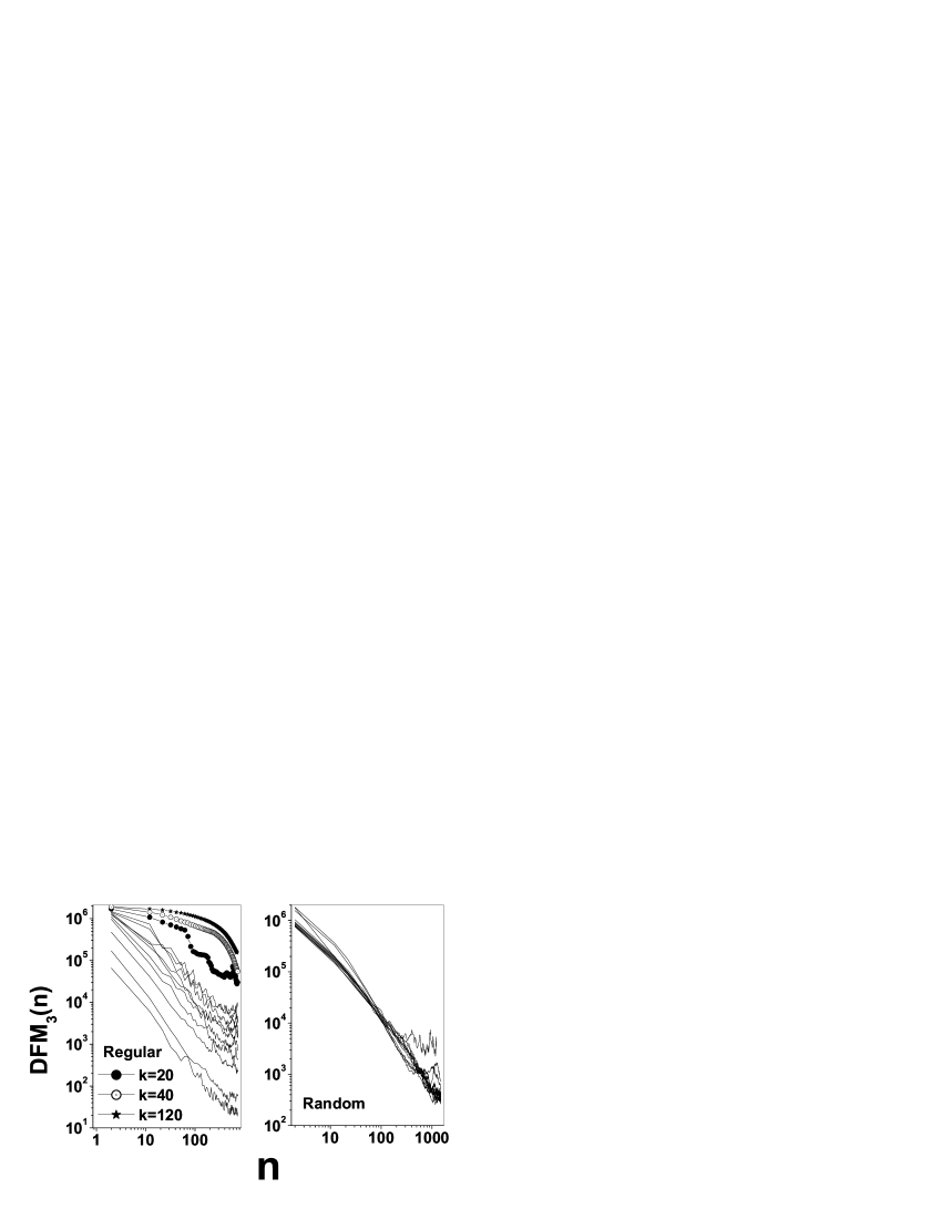
Figure 2: DFM for the two extreme conditions of the WS network model, i.e., regular networks ($p_{r}=0$) and the corresponding completely random networks ($p_{r}=1$). The size of a network $N=3000$. And $q=3$. For these generated networks, when the number of right-handed neighbors $k$ is small ($k=1,2,\cdot\cdot\cdot,9$) the DFMs obey a power-law.

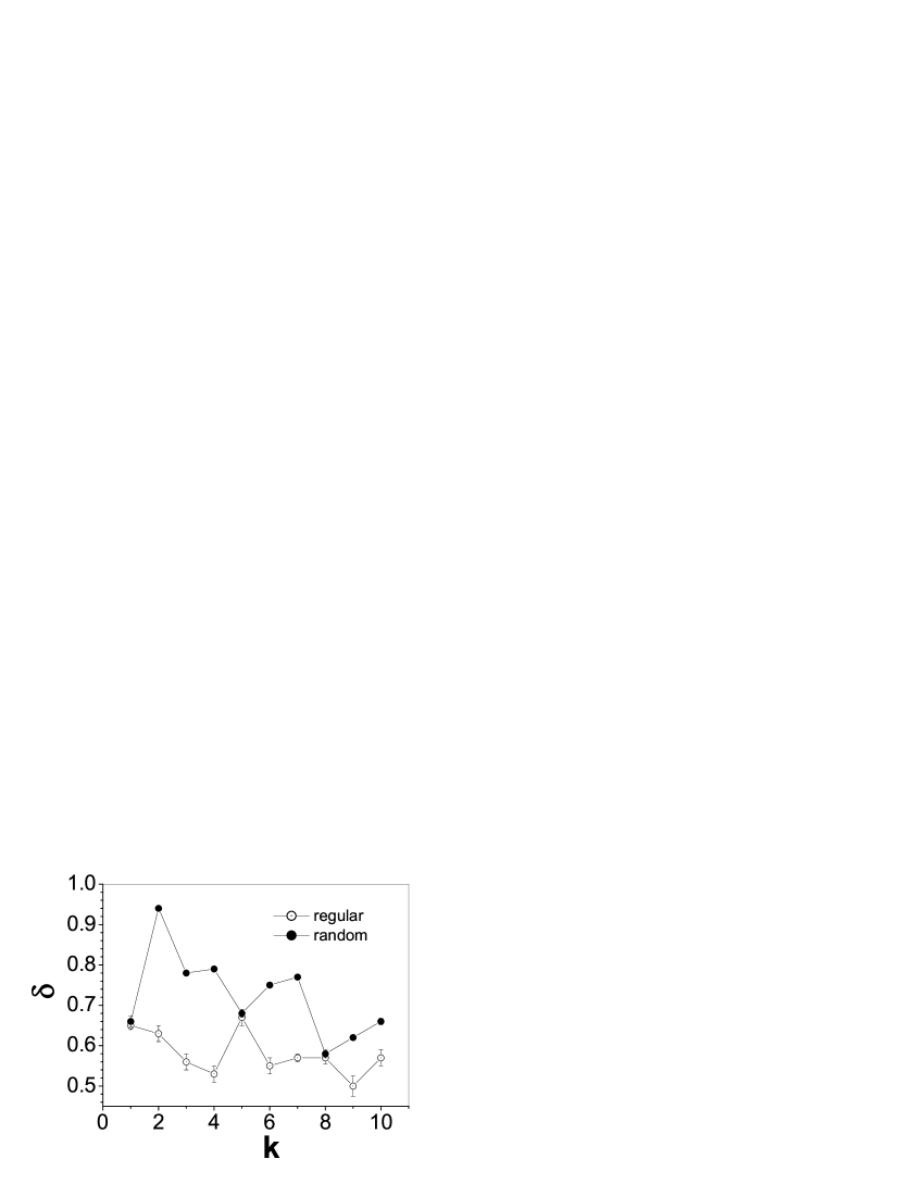
Figure 3: The values of the exponent $\delta$ for the two extreme conditions of the WS network model, i.e, the regular networks ($p_{r}=0$) and the corresponding completely random networks ($p_{r}=1$). The size of a network $N=3000$. And $q=3$. The values of $\delta$ for the regular networks are in the range of $0.58\pm 0.08$, a slight deviation from $0.5$ that corresponds to a Gaussian distribution. The values of $\delta$ for the completely random networks are significantly larger than that of the corresponding regular networks (with a few exceptions).

Fig.2 and Fig.3 show the results for two extreme conditions of the WS network model, i.e., the regular networks with different right-handed neighbors ($p_{r}=0$) and the corresponding completely rewired networks ($p_{r}=1$). When the value of $k$ is unreasonable large ($k=20,40,80,120$), the DFM will not obey a power-law. The scaling exponents for the regular networks are basically in the range of $\delta=0.58\pm 0.08$, a slight deviation from that of the Gaussion distribution. The scaling exponents for the completely rewired networks with $k=2,3,4,6,7$ are significantly larger than that of the corresponding regular networks.

Four typical results for the networks generated with the WS model with different rewiring probability values, as shown in Fig.4, illustrate the significant scale invariance in spectra of these WS networks.The values of $\delta$ for these generated networks with $k=2$ and $k=5$ are presented in Fig5 and Fig.6, respectively. We are specially interested in the rough range of $p_{r}\in[0.05,2]$ where the WS model can capture the characteristics of real world networks. For the generated networks with $k=2$, in the range of $p_{r}\in[0.05,0.2]$ we have $\delta\in 0.71\pm 0.05$. And in the condition of $k=5$, $\delta$ is $0.85\pm 0.05$ in the range of $p_{r}\in[0.1,0.2]$.

Figure 4: Four typical results for WS small-world model. The parameters $q=3$, $k=2$. The size of a network is $3000$ . (a) $p_{r}=0.0$, $\delta=0.67$; (b) $p_{r}=0.1$, $\delta=0.71$; (c) $p_{r}=0.3$, $\delta=0.64$; (d)$p_{r}=0.8$, $\delta=0.80$.

Figure 5: The values of $\delta$ for generated WS networks with different rewiring probabilities. The parameters $q=3,k=2$. In the special range of $p_{r}\in[0.05,0.2]$, where the WS small world network model can capture the characteristics of real world complex networks, we have $\delta\in 0.71\pm 0.05$.

Figure 6: The values of $\delta$ for generated WS networks with different rewiring probabilities. The parameters $q=3,k=5$. In the special range of $p_{r}\in[0.1,0.2]$, where the WS small world network model can capture the characteristics of real world complex networks, we have $\delta\in 0.85\pm 0.05$.

Figure 7: Four typical results for networks generated with the GRN model. The parameter $q=3$. The size of a network is $4000$ . (a) $\theta=0.0$, $\delta=0.88$; (b) $\theta=0.33$, $\delta=0.53$; (c) $\theta=0.5$, $\delta=0.68$; (d)$\theta=1.0$, $\delta=0.86$.

Figure 8: The values of $\delta$ for the networks generated with the GRN model with different $\theta$. At two points $\theta=0.33,0.49$, we have $\delta=0.53$ and $0.52$ (two minimum values), respectively. In the range of $\theta\in[0.33,0.49]$, we have $\delta=0.6\pm 0.1$. And the value of $\delta$ oscillates around $\delta=0.6$ abruptly. In the range of $\theta\in[0.54,1]$, we have basically $\delta>0.7$.

Consider thirdly the growing random network (GRN) model [30,32]. Take several connected nodes as a seed. At each time step, a new node is added and a link to one of the earlier nodes is created. The connection kernel $A_{k}$, defined as the probability that a newly introduced node links to a pre-existing node with $k$ links, determines the structure of this network. The considered complex networks are generated with a class of homogeneous connection kernels, $A_{k}\propto k^{\theta}(0\leq\theta\leq 1)$.

The arguments in literature [32] show that there are two critical points at $\theta_{1}=\frac{1}{3}$ and $\theta_{2}=\frac{1}{2}$, which separate the networks into four groups. The four groups are $\left[{0,\frac{1}{3}}\right)$,$\left({\frac{1}{3},\frac{1}{2}}\right)$,$\frac{1}{2}$and $\left({\frac{1}{2},1}\right)$. From the values of $\delta$ for GRN networks with different $\theta$, shown in Fig.6, we can find that at two points $\theta=0.33,0.49$, we have $\delta=0.53$ and $0.52$ (two minimum values), respectively. In the range of $\theta\in[0.33,0.49]$, we have $\delta=0.6\pm 0.1$. And the value of $\delta$ oscillates around $\delta=0.6$ abruptly. In the range of $\theta\in[0.54,1]$, we have basically $\delta>0.7$.

IV Summary

In summary, we introduced a new concept called DFM and use it to reveal scale invariance features embedded in spectra of complex networks. For an Erdos-Renyi network with connecting probability $p_{ER}<\frac{1}{N}$, the scaling exponent is $\delta=0.5$, while for $p_{ER}\geq\frac{1}{N}$ the scaling exponent deviates from $0.5$ significantly. For the regular networks generated with the WS model with $p_{r}=0$, the scaling exponents deviate slight from $0.5$, the value corresponding to the Gaussian PDF. The other extreme condition is that the $\delta$ values for the random networks generated with the WS model with $p_{r}=1$ are basically significant larger than that for the corresponding regular networks (there are few exceptions). In the specially interested range of $p_{r}\in[0.05,0.2]$, where the WS model can capture the properties of real world networks, the spectra display a typical scale invariance. Two critical points are found for GRN (growing random network) networks at $\theta=0.33$ and $\theta=0.49$, at which we have two minimum values of $\delta=0.53,0.52$, respectively. In the range of $\theta\in[0.54,1]$, we have basically $\delta>0.7$. Hence we find self-similar structures in all the spectra of the considered three complex network models. This common feature may be used as a new measurement of complex networks in a unified way. Comparison with the regular networks and the Erdos-Renyi networks with $p_{ER}<p_{c}=\frac{1}{N}$ tells us that this self-similarity is non-trivial.

The self-similar structures in spectra shed light on the scale symmetries embedded in the topological structures of complex networks, which can be used to obtain the possible generating mechanism of complex networks. Quasicrystal theory tells us that the aperiodic structure of lattice will induce a fractal structure in the corresponding spectrum. The most possible candidate feature sharing by all the complex networks constructed with the three models may be fractal characteristic, which has been proved in a very recent paper [33]. Based upon this feature, we may construct a unified model of complex networks.

- (1) [1] M. E. J. Newman, SIAM Review 45, 167-256 (2003).
- (2) [2] I.J.Farkas, I. Derenyi, A. -L. Barabasi and T. Vicsek, Phys. Rev.E 64, 026704-1(2001).
- (3) [3] M. L. Mehta, Random Matrices, 2nd ed. (Academic, New York, 1991).
- (4) [4] A. Crisanti, G. Paladin, and A. Vulpiani, Products of Random Matrices in Statistical Physics, Springer Series in Solid-State Science Vol. 104 (Springer, Berlin, 1993)
- (5) [5] R. Monasson, Euro. Phys. J. B 12(1999)555.
- (6) [6] I.J. Farkas, I. Derenyi, H. Jeong, Z. Neda, Z.N.Oltvai, E. Ravasz, A.Schubert, A.-L. Barabasi and T. Vicsek, Physica A 314(2002)25.
- (7) [7] K.-I. Goh, B. Kahng and D. Kim, Phys. Rev. E 64,051903(2001).
- (8) [8] K.A. Eriksen, I. Simonsen, S. Maslov and K. Sneppen,Phys. Rev. Lett.90, 148701 (2003); See also , cond-mat/0212001.
- (9) [9] D.Vukadinovic, P. Huang, and T.Erlebach, Lect. Notes Comput, Sci.2346, 83(2002).
- (10) [10] O. Golinelli, Cond-mat/0301437.
- (11) [11] K.Tucci, and M. G. Cosenza, nlin.PS/0312017 v1 8 Dec 2003.
- (12) [12] S. N. Dorogovtsev, A. V. Goltsev, J. F. F. Mendes, and A. N. Samukhin, Phys. Rev. E 68, 046109 (2003); See also, Cond-mat/0306340.
- (13) [13] Huijie Yang, Fangcui Zhao, Longyu Qi and Beilai Hu, Phys. Rev. E 69, 066104(2004).
- (14) [14] Huijie Yang, Fangcui Zhao, Zhongnan Li, Wei Zhang and Yun Zhou, Int. J. Mod. Phys. B 18 (17-19): 2734-2739, (2004).
- (15) [15] Huijie Yang, Fangcui Zhao, Binghong Wang, arXiv:cond-mat/0505086.
- (16) [16] Huijie Yang, Fangcui Zhao, Binghong Wang, to be submitted.
- (17) [17] Nicola Scafetta and Paolo Grigolini, Phys. Rev. E 66036130 (2002).
- (18) [18] G. Paladin, A. Vulpiani, Phys. Rep. 156(1987)147.
- (19) [19] Huijie Yang, Fangcui Zhao, Wei Zhang and Zhongnan Li, Physica A 347(2005)704.
- (20) [20] E. A. De Wolf, Phys. Rep. 270(1996)1.
- (21) [21] A. Bialas, R. Peschanski, Nucl. Phys. B 308(1988)857.
- (22) [22] A. Bialas, R. Peschanski, Nucl. Phys. B 273(1986)703.
- (23) [23] Huijie Yang, Fangcui Zhao, Yizhong Zhuo, Xizhen Wu and Zhuxia Li, Phys. Lett. A 292(2002)349.
- (24) [24] Huijie Yang, Fangcui Zhao, Yizhong Zhuo, Xizhen Wu and Zhuxia Li, Physica A 312(2002)23.
- (25) [25] http://soi.stanford.edurmunk/Propack/Propack.tar.gz.
- (26) [26] P. Erdos, A. Renyi, Publ. Math. Inst. Hung. Acad. Sci. 5, 17(1960); B. Bollobas, Random Graphs (Academic Press, London, 1985).
- (27) [27] D. Stauffer and A. Aharony, Percolation Theory (Taylor& Francis, London, 1992).
- (28) [28] D.J. Watts and S.H. Strogatz, Nature (London) 393, 440(1998).
- (29) [29] D.J. Watts, Small Worlds: The dynamics of Networks Between Order and Randomness (Princeton Reviews in Complexity) (Princeton University Press, Princeton, NJ, 1999).
- (30) [30] A. -L. Barabasi and R. Albert, Science 286,509(1999).
- (31) [31] A. -L. Barabasi and R. Albert, H. Jeong, Physica A 272, 173(1999).
- (32) [32] P. L. Krapivsky, S. Redner, and F. Feyvraz, Phys. Rev. Lett. 85, 4629-4632 (2000). See also, arXiv: cond-mat/0005139 v2 18 Sep 2000.
- (33) [33] Chaoming Song, Shlomo Havlin, Hernan A. Makse, Nature,433, (2005), 392-395.