Implications of the Low-Temperature Instability of Dynamical Mean Theory for Double Exchange Systems

Abstract

The single-site dynamical mean field theory approximation to the double exchange model is found to exhibit a previously unnoticed instability, in which a well-defined ground state which is stable against small perturbations is found to be unstable to large-amplitude but purely local fluctuations. The instability is shown to arise either from phase separation or, in a narrow parameter regime, from the presence of a competing phase. The instability is therefore suggested as a computationally inexpensive means of locating regimes of parameter space in which phase separation occurs.

I Introduction

Dynamical mean field theory (DMFT) has been widely applied to many strongly correlated electron systemsGeorges . Since DMFT takes local quantum fluctuations into account, it is especially successful for models whose many body effect comes from the on-site interaction, like HubbardHubbard or KondoKondo Chattopadhyay (double exchange) model. Correlated systems often exhibit different phases which are quite close in energy, and this proximity can lead to phase separation, which is often important for electronic physicsDagotto2 . Phase separation is in principle a ”global” property of the phase diagram and requiring substantial effort to establish: one must compute the free energy over a wide parameter range, and then perform a Maxwell construction. In this paper we show that within the single-site DMFT formalism a straightforward calculation at a fixed parameter value can reveal the presence of phase separation. Specifically, we find that at zero temperature, the DMFT can give a ground state which is stable against small perturbations but is unstable to a large amplitude local perturbation; at non-zero temperature the standard methods simply fail to converge to a stable solution. By computing the free energy and performing a Maxwell construction we show that for wide parameter ranges this instability occurs in the regions in which phase separation exists. In a narrow parameter regime it signals instead the onset of a different, but apparently uniform, phase. We therefore propose that the instability of the DMFT equations can be used as an approximate, computationally convenient estimator for the boundaries of the regimes in which phase separation occurs.

The balance of this paper is organized as follows. We first present the model and then a zero temperature dynamical mean field analysis explicitly showing the instability. In section III we calculate the full T=0 phase diagram in the energy-density plane, establish the regime of phase separation via the usual Maxwell construction, and extend the treatment to $T>0$. In section IV we discuss the implications of this instability. Finally in section V we present a brief conclusion.

II Double Exchange Model and Dynamical Mean Field Approximation

II.1 Double Exchange Model

In this paper, we consider the single orbital ”double exchange” or Kondo lattice model of carriers hopping between sites on a lattice and coupled to an array of spins. This model has been studied by many authors and contains important aspects of the physics of the ”colossal”Colossal magnetoresistance manganites and is also solvable in a variety of approximations, permitting detailed examination of its behavior. Here we use it to investigate the physical meaning of a previously unnoticed instability of the dynamical mean field equations.

The model is defined by the Hamiltonian

$$H = \sum_{\sigma,i,j}t_{ij}(c^{+}_{i,\sigma}c_{j,\sigma}+h.c.)+\sum_{i,\alpha,\beta}J\vec{S}_{i}\cdot c^{+}_{i,\alpha}\,\vec{\sigma}_{\alpha\beta}\,c_{i,\beta}$$

with $i,j$ labeling the sites and the $\vec{S}_{i}$ denoting the spins. We assume the spins are classical ($\left[{\vec{S}}_{i},{\vec{S}}_{j}\right]=0$) and are of fixed length. We choose the convention $|\vec{S}_{i}|=1$.

The hopping $t_{ij}$ defines an energy dispersion $\varepsilon_{k}$ and thus a density of states $D(\varepsilon)=\int d^{d}k/(2\pi)^{d}\delta(\varepsilon-\varepsilon_{k})$. In our actual computations we specialize to the $d\rightarrow\infty$ limit of the Bethe lattice, for which $D(\varepsilon)=\sqrt{4t^{2}-\epsilon^{2}}/(2\pi t^{2})$ because the availability of convenient analytical expressions allows us to accurately compute the small difference between free energies of different states. We choose energy units such that $t=1$.

We also note that the ground state properties of the model may be straightforwardly obtained, because for any fixed configuration of the spins the model is quadratic in the fermions and easily diagonalizable.

II.2 Dymanical Mean Field Method

We now present the dynamical mean field analysis of this model. In the single site dynamical mean field methodGeorges , one neglects the momentum dependence of the self energy. The properties of the model may then be calculated by solving an auxiliary quantum impurity model, along with a self consistency condition. The quantum impurity model corresponding to Eqn(LABEL:Eqs:H) is specified by the partition function

$$Z_{imp}=\int\,d\vec{S}\,e^{{\cal A}}$$ (2)

with ${\cal A}=\mbox{Tr}\log\left[a_{\uparrow}a_{\downarrow}-J\cos\theta(a_{\uparrow}-a_{\downarrow})-J^{2}\right]$ where the trace is over frequency, and $\cos\theta=\hat{z}\cdot\vec{S}$. $S$ is determined by a spin-dependent mean field function $a(\omega)$. In a magnetic phase, $a_{\uparrow}\neq a_{\downarrow}$. Note that the assumption of classical core spins means that $\int\,d\vec{S}$ denotes a simple scalar integral over directions of the core spin $\vec{S}$, and that no Berry phase term occurs in the argument of the exponential.

The Green function $G_{imp}$ and self energy $\Sigma(\omega)$ of the impurity model are given by

$$G_{imp,\sigma}(\omega) \equiv \frac{\delta\log Z_{imp}}{\delta a_{\sigma}(\omega)}$$

$$\Sigma_{\sigma}(\omega) \equiv a_{\sigma}-G_{imp,\sigma}^{-1}$$ (3)

$a$ is fixed by requiring the impurity Green’s function $G_{imp}$ equals to the local Green’s function of the lattice problem. The form of the self consistency equation depends on the state which is studied. For a ferromagnetic (FM) state, it is

$$G_{imp,\sigma}=\sum_{\vec{k}\subset\mbox{BZ}}(\omega+\mu-\epsilon_{\vec{k}}-\Sigma_{\sigma}(\omega))^{-1}$$ (4)

while for a 2 sublattice antiferromagnetic (AF) state,

$$G_{imp,\sigma}=\sum_{\vec{k}\subset\mbox{RBZ}}\left(\begin{array}[]{cc}\xi_{1}&-\epsilon_{\vec{k}}\\ -\epsilon_{\vec{k}}&\xi_{2}\end{array}\right)^{-1}$$ (7)

where $\xi_{1\,(2)}=i\omega_{n}+\mu-\Sigma_{\uparrow\,(\downarrow)}$ and the $\vec{k}$ -sum is over tje reduced Brillouin zone (RBZ). The two equations become equivalent in the paramagnetic (PM) state where $\Sigma_{\uparrow}=\Sigma_{\downarrow}$

The solution of Eqs [3 to 7] determines the magnetic phase, the single particle properties, and the free energy. In particular, in the dynamical mean field approximation the Gibb’s free energy is Georges FE

$$\frac{\Omega}{N}=\Omega_{imp}-T\mbox{Tr}\log G_{\sigma}(i\omega_{n})-T\mbox{Tr}\log G^{-1}_{\sigma}(i\omega_{n},\vec{k})$$ (8)

where the trace is over the spin and lattice degree of freedom. The Helmholtz free energy is $F(n)=\Omega+\mu\,N$. At zero temperature, the ground state energy (Helmholtz free energy) is

$$\frac{E}{N}=\mbox{Tr}[G(i\omega_{n},\vec{k})(i\omega_{n}+\mu)]$$ (9)

We also note that the solution $a_{\sigma}(i\omega_{n})$ defines an effective potential for the core spin, which depends on the angle $\theta$ between the core spin and local magnetization direction, so that

$$Z_{imp}\rightarrow Z_{0}\int\,d\cos\theta\,e^{-E_{eff}(\cos\theta)/T}$$ (10)

with

$$E_{eff}(\cos\theta)=-T\sum_{i\omega_{n}}\log\left[1-\frac{J\cos\theta(a_{\uparrow}-a_{\downarrow})+J^{2}}{a_{\uparrow}a_{\downarrow}}\right]$$ (11)

II.3 Phase Boundaries and Maxwell Construction

The model is known to exhibit ferromagnetic, spiralSpiral and commensurate antiferromagnetic phases. For our subsequent analysis, an accurate determination of phase boundaries will be important. We therefore present here a few calculational details.

We require the $T=0$ phase boundary separating the ferromagnetic and spiral phasesChattopadhyay Spiral . The energy of a spiral state may most easily be found by performing a site-dependent spin rotation to a basis in which the spin quantization axis is parallel to the local spin orientation. The problem may then be easily diagonalized. For the infinite dimensional Bethe lattice one finds, for a diagonal spiral of pitch $\phi$, that in the rotated basis, the local Green function is given byChattopadhyay

$$\tilde{G}^{-1}_{\sigma}(\omega)=\omega+\mu-\sigma J-t^{2}\cos^{2}(\frac{\phi}{2})\tilde{G}_{\sigma}-t^{2}\sin^{2}(\frac{\phi}{2})\tilde{G}_{\bar{\sigma}}$$

where $\phi$ is the angle between two nearest neighbor magnetization, and tilde is used for the spiral states.

To locate the $T=0$ FM/spiral second order phase boundary, it suffices to expand ground state energy $E(\mu,\phi)$ (Eqn(9)) to second order in $\phi$. The energy difference between FM and spiral states is

$$dE|_{N}=\frac{\partial\Omega}{\partial\phi}d\phi=\left(\frac{\phi}{2}\right)^{2}\,T\sum_{n}i\omega_{n}\,dG(i\omega_{n},\mu)$$ (13)

with $dG$ equaling to

$$d\,G_{\sigma}=\tilde{G}_{\sigma}-G_{\sigma}=\frac{t^{2}\left(G_{\sigma}-G_{\bar{\sigma}}\right)}{t^{2}-G_{\sigma}^{-2}}$$ (14)

where $\bar{\sigma}=-\sigma$. The FM/spiral phase boundary is determined by $dE|_{N}=0$.

Figure 1: Energy as function of particle density at $J=1$, $T=0$, illustrating Maxwell construction. Heavy solid line: FM state. Light solid line: 2 sublattice AF state. Dashed line: Maxwell construction interpolatiion.

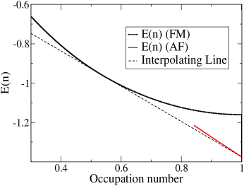
The model also exhibits phase separation in some regimes. To determine the boundaries of the regime where phase separation occurs, we use the DMFT method to compute the Helmholtz free energy as a function of occupation number $F(n)$ (Eqn(8)) and then perform the Maxwell construction. An example is shown in Fig 1. We find that in fact that over much of the phase diagram a phase separation between FM and $n=1$ AF states preempts the formation of spiral or $n<1$ AF state. The general structure of our phase diagram agrees with earlier workDagotto Guinea , but the precise locations of phase boundaries differ by roughly $10\%$.

III DMFT Instability

(a) FM Instability

(b) AF Instability

Figure 2: (a) Effective potential for the core spin (Eqn(11)) for a ferromagnetic state calculated at $T=0$, $J=8$, and densities shown. As we increase the occupation number from 0.88 to 0.90, the minimum of $E_{eff}(\cos\theta)$ changes from $\cos\theta=-1$ to 1 which indicates the FM DMFT solution becomes unstable when $n>0.89$. (b) Effective potential for the core spin for an anti-ferromagnetic state calculated at $T=0$, $J=1$, and densities shown. At $n=1$, the minimum of $E_{eff}$ happens at $\cos\theta=-1$, while at $n=0.995$ the minimum changes to $\cos\theta=1$. The AF DMFT solution only exists at $n=1$.

In this section we show that the DMFT equations exhibit an apparently previously unnoticed instability. We begin with $T=0$. From Eqn(3), the $G_{imp}$ is

$$G_{imp,\uparrow(\downarrow)}=<\frac{a_{\downarrow(\uparrow)}-(+)J\cos\theta}{a_{\uparrow}a_{\downarrow}-J\cos\theta(a_{\uparrow}-a_{\downarrow})-J^{2}}>$$ (15)

where $<...>$ means the angular average with respect to the weight function $e^{-E_{eff}(\cos\theta)/T}$, with $E_{eff}$ defined in Eqn(11) . At zero temperature, the only contribution of the angular average is from the absolute minimum of $E_{eff}(\cos\theta)$. To find the DMFT solution at $T=0$, one first assumes the absolute minimum of $E_{eff}(\cos\theta)$ occurs at a fixed value, for example $\cos(\theta)=-1$, obtains $G_{imp,\uparrow(\downarrow)}^{-1}=a_{\downarrow(\uparrow)}-(+)J$ from Eqn(15), and gets the self energy $\Sigma_{\uparrow\,(\downarrow)}=+(-)J$ from Eqn(3). Finally, one uses the $a$ obtained by the above procedure to calculate $E_{eff}(\cos\theta)$ to see if the minimum is located at the point originally assumed. Note that different ground states (FM, AF..) enter the above procedure only via the self consistent equation Eqn(4) (or Eqn(7)).

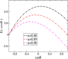
Fig 2 shows that as density is increased at fixed large $J$, the self consistency breaks down, in an unusual manner: $E_{eff}(\cos\theta)$ remains locally stable (slope around the assumed minimum $\cos(\theta)=-1$ remains positive) but the global minimum of $E_{eff}$ moves to $\cos(\theta)=1$. In the regime where this phenomenon occurs, no solution of the DMFT equations exists. Any initial solution we have considered leads to a similar inconsistency (as is shown in panel b of Fig2 for the case of anitferromagnetism).

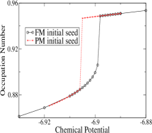
This instability is also manifest at $T>0$. As $T$ is decreased at fixed $n$, the convergence becomes slower and below some temperature $T^{*}(n)$, no stable solution can be found for a $J$-dependent range of $n$. The absence of a solution for some range of $n$ can be seen in a different way by solving the model as a function of chemical potential $\mu$ Fig 3(a) shows that as $\mu$ is increasedat fixed low $T$, a first order transition occurs to a paramagnetic state, with a corresponding jump in $n$. Associated with the first order transition is a coexisting region in which two solutions are locally stable (FM with lower $n$ and PM with higher $n$); the DMFT equations correspondingly have two solutions, which one is found depends on the initial seed. The solid and dashed lines in Fig 3(a) are obtained from initial seeds close to FM and PM states respectively.

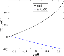
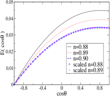
The absence of convergence may be understood from the density dependent effective potential, shown e.g. in Fig 3(b). One sees that as $n$ is increased, $E(\cos\theta=1)$ decreases; this is a precursor of the effect shown in Fig 2(a). Indeed, the curve $E(\cos\theta)$ is reduced by an $n$-dependent scale factor. For $n$ larger than a critical value (here $n\sim 0.905$), $E(\cos\theta=1)$ is small enough relative to the temperature that this region begins to contribute to $<\cos\theta>$, lowering the maximum $m$ that can be sustained and destabilizing the ferromagnetic solution.

Figure 3: (a) $n(\mu)$ at $J=8$ and $T=0.01$, showing two phase behavior. Solid line: obtained from the initial seed close to the FM state. Dashed line: obtained from the initial seed close to the PM state. (b) $E_{eff}(\cos\theta)$ at $J=8$, $T=0.01$, $n=0.88$(solid line), 0.89 (dot line), and 0.90(dashed line). The circle and dagger represent the scaled effective potential for $n=0.88$ and 0.89 which are almost indistinguishable to the $E_{eff}$ at $n=0.90$.

Figure 4: (a) $T=0$ phase boundaries. Solid line: DMFT instability above which the DMFT solution becomes unstable Dot line: spiral instability line. The system is spiral(FM) above(below) this line. Dashed line: AF/FM phase separation. (b) Expansion of the region $0.8t<J<2t$. For $n$, $J$ in the triangle bounded below by the solid line and above by the dashed and dot lines, the ground state is not known.

Figure 5: (a) Phase Boundaries for J=8 in $n-T$ plane. Solid line: the phase separation boundary obtained by Maxwell construction. Dotted line: Curie temperature. Dashed line: the boundary of DMFT instability. (b) Maxwell construction for $J=8$, $T=0.008$ – the difference between free energy and interpolating line. The ground state is FM when $n<0.86$, and FM/AF phase separaion for $0.86<n<1$.

IV Interpretation

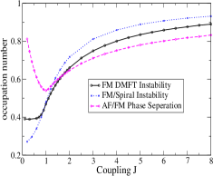
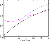
We argue in this section that the DMFT instability documented in the previous section is a manifestation of competing instabilities (primarily phase separation) in the original model. To establish this we show in the panel (a) of Fig 4 a $T=0$ phase diagram in the density-coupling plane. The dash-dot line shows the phase separation boundary obtained from the global energy computation; for $n$ above this line the model phase separates into an $n=1$ AF and an $n<1$ FM state. The dotted line shows the phase boundary between uniform FM and spiral states. Finally, the heavy solid line shows the region above which the FM DMFT solution is unstable at $T=0$. When $J$ is large enough that the FM state is fully polarized ($J>2t$), we see that the DMFT instability line follows the phase separation line, but is inside the region of phase separation. We therefore suggest that in this region the DMFT instability is a consequence of phase separation and this DMFT instability line can be used as a rough estimate of the real phase separation boundary.

When $J<0.8t$, the DMFT instability indicates the presence of a spiral state with lower energy than the ferromagnetic state. For $0.8t<J<1.7t$ (Fig 4(b)), there exists a narrow region of $n$ where none of the uniform phases we considered solve the DMFT equations and the Maxwell constructions seem not to indecate phase separation. We believe that in this region there exists a uniform non FM/AF/spiral/paramagnetic state (either the ground state or the phase separation beteen FM and that state) which we do not know yet.

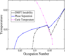
At $T>0$ the situation is similar. The DMFT instability is contained inside the regime of phase separation. For example, we show in Fig 5(a) the phase diagram and the range of DMFT instability in the density-temperature plane for $J=8t$. The heavy line shows the boundary of the regime of phase separation obtained by Maxwell construction: for $0<T<0.011$, the phase separation is between FM and AF($n=1$); for $0.012<T<0.02$, the phase separation is between PM and AF($n=1$); for $0.011<T<0.012$, the phase separation is either PM-AF($n=1$) or FM-PMFM-PM according to the location $n,T$ relative to the homogenous Curie temperature (dotted line). The dashed line shows the region where the DMFT solution fails to converge at that given density $n$ (the DMFT equation has stable solution for all $\mu$, see Fig 3(a)). For $n>0.95$, the DMFT instability line denotes the temperature below which (a) the paramagnetic state is linearly unstable to antiferromagnetic and (b) no stable antiferromagnetic solution exists (except $n=1$).

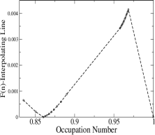
Fig 5(b) shows the results of a Maxwell construction for $J=8$ and that at $T=0.008$, presented as the difference between calculated free energy $F(n)$ and the interpolating line $I(n)=F(n=1)+\frac{F(n^{*})-F(n=1)}{1-n^{*}}(1-n)$ with $n^{*}=0.86$. Phase separation is seen to occur for $n^{*}<n<1$, while the DMFT instability range is $0.895<n<0.95$ and $0.96<n<1$.

V Conclusion

We have found an instability in the ferromagnetic DMFT equation for the single site double exchange model and shown that this instability corresponds to the FM/AF phase separation when the coupling $J$ is larger than half bandwidth (2$t$) and to another ground state (spiral) in the small coupling region. There exists a small window, around intermediate $J$, where no stable FM DMFT solutions exist while the spiral or phase separation is not the ground state, and we believe there is a non FM/AF/Spiral/Para ground state existing in this region. We have presented evidence that the instability is a signal, obtained from a calculation at a fixed parameter value, of the existence of an instability (typically phase separation) which normally is established via a global computation, comparing free energies at many different parameter values. We therefore propose that the DMFT instability is a computationally convenient way to estimate the boundary of phase separation.

We thank Dr. Satoshi Okamoto for many helpful discussions. This work is supported by DOE ER46169 and Columbia University MRSEC.

References

- (1) A.Georges, G.Kotliar, W.Krauth, and M.Rozenberg, Rev of Modern Physics 68, 13 (1996)
- (2) A.Georges, and W. Krauth, Phys.Rev.Lett 69, 1240 (1992). M.J. Rozenberg, G.Kotliar, amd X.Y. Zhang, Phys.Rev.Lett 69, 1236 (1992).
- (3) A. J. Millis, R. Mueller, and Boris I. Shraiman Phys. Rev. B 54, 5389 (1996). A. J. Millis, R. Mueller, and Boris I. Shraiman Phys. Rev. B 54, 5405 (1996).
- (4) A.Chattopadhyay, A.J.Millis, and S. Das Sarma Phys.Rev.B. 64, 012416-1 (2001)
- (5) E.Dagotto Sience 309, 257 (2005)
- (6) See, e.g. the articles in Colossal Magnetoresistive Oxides, Y.Tokura,ed (Gordon and Breach: Tokyo, 1999)
- (7) In Eqs(8), for FM and AF states, the lattice Green function are indicated in Eqn(4) and Eqn(7), while the trace are over full and reduced Brillouin zone respectively.
- (8) J.Inoue and S.Maekawa Phys.Rev.Lett 74, 3407 (1995).
- (9) S.Yunoki, J.Hu, A.L.Malvezzi, A.Moreo, N.Furukawa, and E.Dagotto Phys.Rev.Lett 80, 845 (1998).
- (10) D.P.Arovas, G.Gomez-Santos, F.Guinea, Phys.Rev.B. 59, 13569 (1999)
- (11) The precise boundary of PM-FM phase separation is hard to determine because it is very close to the FM DMFT instability line. They coincide within our numerical error.