Phase separation of a model binary polymer solution in an external field.

Abstract

The phase separation of a simple binary mixture of incompatible linear polymers in solution is investigated using an extension of the sedimentation equilibrium method, whereby the osmotic pressure of the mixture is extracted from the density profiles of the inhomogeneous mixture in a gravitational field. In Monte-Carlo simulations the field can be tuned to induce significant inhomogeneity, while keeping the density profiles sufficiently smooth for the macroscopic condition of hydrostatic equilibrium to remain applicable. The method is applied here for a simplified model of ideal, but mutually avoiding polymers, which readily phase separate at relatively low densities. The Monte-Carlo data are interpreted with the help of an approximate bulk phase diagram calculated from a simple, second order virial coefficient theory. By deriving effective potentials between polymer centres of mass, the binary mixture of polymers is coarse-grained to a “soft colloid” picture reminiscent of the Widom-Rowlinson model for incompatible atomic mixtures. This approach significantly speeds up the simulations, and accurately reproduces the behaviour of the full monomer resolved model.

I Introduction

Polymer solutions segregate into polymer-rich and polymer-poor phases when the temperature is lowered below the theta-point. Polymer blends nearly always demix in the melt, because the connectivity constraints strongly reduce the entropy of mixingrubin . Less is known, however, about the phase behaviour of dilute or semi-dilute polymer solutions involving two or more polymeric species. In particular, the quality of the solvent is generally not the same for different polymeric species, which may lead to competing mechanisms in the subtle free-energy balance between entropic and energetic contributions. In the case of binary mixtures of incompatible polymers in a common good solvent, excluded volume effects lead to strong deviations from mean-field behaviourbroseta ; sariban . In this paper we consider a highly simplified model of mutually repelling polymer in a common $\theta$ solvent. The system under consideration extends the familiar Widom-Rowlinson modelwidom for incompatible atomic mixtures to polymer blends in solution. Not surprisingly, the mutual incompatibility of the two species in the athermal model leads to demixing above a critical density. The additional feature introduced in the present work is the presence of an externally applied field, specifically a gravitational field, acting on the polymers, which induces a spatial inhomogeneity.

The interest of the applied field is two-fold. The first is essentially methodological: as we have shown recently for cases of single-component polymer solutionsadd2 and of di-block copolymer solutions add3 , the density profiles characterising the inhomogeneous distribution of polymers may be exploited to extract the osmotic equation-of-state over a wide range of concentrations in a single simulationbiben . A second motivation is that applying an external field allows us to rapidly search through phase space to locate phase-transitions, although it must be kept in mind that adding a field affects the phase behaviour, as demonstrated in a recent theoretical investigations of colloid-polymer mixturesschmidt .

Finally, we demonstrate in this paper the merits of coarse-grained representations of complex polymeric systems, whereby the total number of degrees of freedom is drastically reduced by tracing out individual monomer coordinates to determine effective interactions acting between polymer centres of mass. This strategy has proved very successful for solutions of linear polymersdaut ; bolh ; bolh2 , mixtures of asymmetric star polymersMaye04 , di-block copolymersadd3 and is extended here to linear polymer mixtures, in an effort to map out their phase diagram. Our coarse-graining strategy is similar in spirit to that successfully applied by the Klein group to surfactants and other self-assembling systemsNiel04 .

II Model and methodology

Consider a binary polymer mixture of linear homopolymers with $M_{A}$ and $M_{B}$ monomers respectively. For computational purposes the two species are assumed to ”live” on a cubic lattice of $L_{x}\times L_{y}\times L_{z}$ sites. Monomers occupy lattice sites, and the lattice spacing coincides with the segment length $b$. Let $N_{A}$ and $N_{B}$ be the total numbers of polymers of the two species. The overall polymer densities (coils per unit volume) are $\rho_{\alpha}=N_{\alpha}/V$, where $V=L_{x}L_{y}L_{z}b^{3}$ (we set $b$ to $1$ in this paper). An external force field along the $z$-direction, acting on monomers of each species $\alpha$, and deriving from the potential $\psi_{\alpha}(z)(\alpha=A$ or $B$) will induce an inhomogeneity in the mixture characterised by two density profiles $\rho_{\alpha}(z)$. Alternatively, one may define the overall polymer density $\rho(z)=\rho_{A}(z)+\rho_{B}(z)$ and the concentration ratio profile:

$$x(z)=\rho_{A}(z)/\rho(z)$$ (1)

The density profiles are normalised such that:

$$\int_{0}^{L_{z}}\rho_{\alpha}(z)dz=n_{\alpha}=\frac{N_{\alpha}}{L_{x}L_{y}}$$ (2)

If the inhomogeneity induced by the external field varies sufficiently slowly in space, the binary mixture obeys the hydrostatic equilibrium condition:

$$\frac{dP(z)}{dz}=-\rho_{A}(z)\frac{d\psi_{A}(z)}{dz}-\rho_{B}(z)\frac{d\psi_{B}(z)}{dz}$$ (3)

where $P(z)$ is the local osmotic pressure of the binary polymer mixture in solution. The macroscopic conditionsariban may be shown to follow from the “local density approximation” (LDA) within density functional theory of inhomogeneous fluidsbiben . If the profiles $\rho_{A}(z)$ and $\rho_{B}(z)$ are computed in Monte-Carlo (MC) simulations of binary mixtures subjected to the external field, $P(z)$ may be determined by integration of equation 3. The equation-of-state of the inhomogeneous mixture along an isotherm, $P(\rho_{A},\rho_{B})$ or $P(\rho,x)$ may then be extracted by eliminating the altitude $z$ between $P(z),\rho_{A}(z)$ and $\rho_{B}(z)$ (or $\rho(z)$ and $x(z)$).

In practice, the external field is chosen to be the gravitational field acting on the centre-of-mass of the polymers:

$$\psi_{\alpha}(z)=M_{\alpha}m_{\alpha}gz$$ (4)

where $m_{\alpha}$ is the buoyant mass of monomers of species $\alpha$ and g is the acceleration due to gravity. Since gravity acts as a confining field, it is convenient to take $L_{z}\rightarrow\infty$. Although, under normal experimental conditions, gravity is insufficient to induce significant inhomogeneity in a polymer solution, (ultra-centrifugation would be required to induce a measurable effect) here gravity may be tuned at will in simulations to achieve sedimentation lengths $\zeta=k_{B}T/m_{\alpha}g$ comparable to radii of gyration $R_{g\alpha}$, and hence a significant variation of the density profiles.

Substitution of equation 4 into equation 3 and integration leads to :

$$P(z)/k_{B}T=1/\zeta_{\alpha}\int_{z}^{\infty}\rho_{\alpha}(z^{\prime})dz^{\prime}+1/\zeta_{\beta}\int_{z}^{\infty}\rho_{\beta}(z^{\prime})dz^{\prime}.$$ (5)

The equation-of-state $P(\rho_{\alpha},\rho_{\beta})$ of the heterogeneous mixture may thus be determined from the density profiles $\rho_{\alpha}(z)$ and $\rho_{\beta}(z)$ as explained above. In practice MC runs are carried out for several overall concentrations, in order to map out the complete equation-of-state. It is important to realise that, in general, not only the overall density $\rho(z)$, but also the concentration $x(z)$ varies with altitude, as may be easily verified for the simple case of a binary mixture of ideal (non-interacting) polymers.

We have applied the hydrostatic equilibrium method to a very simple non-trivial model of a binary polymer mixture which demixes in solution. In the model A and B polymers freely penetrate coils of the same species, i.e. follow random walk statistics, while A-B pairs experience excluded volume between their monomers i.e. behave like mutually avoiding walks. The model is one of a family of six XYZ models, where X, Y, and Z label the statistics of A-A, A-B and B-B interaction pairs. Thus each of X, Y, and Z can take one of two “values”, I for ideal (non-interacting) and S for self (or mutually) avoiding. In particular SSS refers to a binary mixture of polymers in which all interactions are self avoiding, i.e. a homogeneous solution of SAW polymers, while the model under consideration here is the ISI model. Note that the ISI model generalises the familiar Widom-Rowlinson modelwidom to polymer mixtures; a related block co-polymer model, where A and B are tethered, has recently been investigated by our groupadd3 . While the latter leads to micro-phase separation, the present binary ISI model is expected to undergo bulk phase separation due to the incompatibility of the A and B components. For the sake of simplicity, the following investigations are restricted to the case of equal length polymers ($M_{A}=M_{B}=M$). Moreover, without loss of generality, the monomer masses may be assumed to be equal ($m_{A}=m_{B}=m$), so that $\zeta_{A}=\zeta_{B}=\zeta$. Note that this model is athermal. Polymers were subjected to pivot and translational MC moves, typically $1\times 10^{6}-1\times 10^{8}$ MC moves per polymer.

III Coarse-grained description

Following a known strategydaut ; bolh ; bolh2 , one can calculate effective interactions $v_{\alpha\beta}(r)$ between CMs of A-A, A-B and B-B pairs, by averaging over the conformations of two polymers for fixed values of the distance $r$ between their CMs. Explicitly, for an isolated pair of A and B polymers:

$$v_{\alpha\beta}(r)=-k_{B}TlnP_{AB}(r)$$ (6)

where $P_{AB}(r)$ is the probability (averaged over all random walk configurations of the two polymers) that there is no overlap between monomers of A and monomers of B when their CMs are held at a distance $r$. Obviously $v_{AA}(r)=v_{BB}(r)=0$ for the ISI model, since like-species overlaps are allowed. Effective pair potentials like $v_{AB}$ in eq. 6 are easily computed in MC simulation, as explained on more detail in the referencesbolh ; bolh2 .

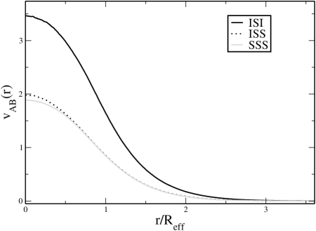
Figure 1: Effective potential $v_{AB}(r)$, in units of $k_{B}T$, between the centres of mass of two polymers for ISI, ISS and SSS models. These potentials were generated at zero density using Monte Carlo simulations of two $L=500$ polymers on a simple cubic lattice.

Examples are shown in figure 1 for the ISI, ISS and SSS models; since the two species are of equal length, the SSS model is equivalent to a one-component system of self-avoiding walk (SAW) polymers, which has been thoroughly investigatedbolh ; bolh2 ; pelis . While the potentials $v_{AB}(r)$ for the SSS and ISS models are very close, the effective potential for the ISI model is considerably more repulsive,with a value at full overlap, $v_{AB}(r=0)\simeq 3.45k_{B}T$. This enhancement of the effective repulsion may be easily understood by noting that the A and B coils are more compact (their radii of gyration are those of ideal chains, which scale as $R_{g}\sim M^{0.5}$, as compared to chains with SAW internal statistics, which scale as $R_{g}\sim M^{0.59}$). Hence the overlap probability is higher (i.e. $P_{AB}(r)$ is lower) in the former compared to the latter case, for any given $r/R_{eff}$ where the effective radius is defined by

$$R{{}^{2}}_{eff}=\frac{1}{2}(R_{gA}{{}^{2}}+R_{gB}{{}^{2}}).$$ (7)

The second virial coefficient for the ISI model may be calculated from $v_{AB}(r)$ according to:

$$B_{AB}=-2\pi\int_{0}^{\infty}(e^{-v_{AB}(r)/k_{B}T}-1)r^{2}dr$$ (8)

and turns out to be $B_{AB}\simeq 9.5R_{g}^{3}$ for our $L=500$ ISI model lattice polymers.

It has been shownbolh that the effective pair potential between linear SAW polymers varies significantly as the polymer density is increased from the infinite dilution limit, particularly so beyond the overlap density $\rho^{*}=3/4\pi R_{g}^{3}$. This effect is expected to be less important for the ISI model, since it will be shown that phase separation, which leads to a dramatic reduction of the number of A-B contacts, sets in for $\rho$ greater than $\sim\frac{1}{2}\rho^{*}$.

IV Equation-of-state of the symmetric mixture

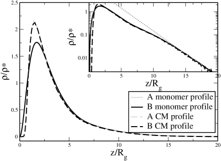
Figure 2: The centre of mass and monomer density profiles for the symmetric equimolar ISI model, with the same profiles on a logarithmic scale shown as an insert. These profiles were generated from simulations of $1600$ polymers of length $L=500$ in a box with a base of $L_{x}=L_{y}=200$ that is open in the positive $z$ direction, along which the density profiles are plotted. The dashed line on the logarithmic scale (inset) shows the exponential behaviour of ideal polymers $\rho(z)\sim\exp(-z/\zeta)$, with the gravitational length $\zeta=2.19R_{g}$.

In order to determine the full equation-of-state $P(\rho_{A},\rho_{B})$ or $P(\rho,x)$ by the hydrostatic equilibrium method presented in section 2, simulation of the ISI model must be carried out on systems involving several overall compositions. In the equimolar case, the ISI model is fully symmetric with respect to the A and B species, so that the local concentration $x(z)$ remains constant (equal to $x=\frac{1}{2}$) at all altitudes. Examples of MC-generated monomer and CM density profiles $\rho_{A}(z)$ and $\rho_{B}(z)$ of the equimolar ISI model are shown in figure 2. As expected, the density profiles of the two species are identical within statistical errors. The two profiles exhibit a depletion zone (which is more pronounced for the CM profile) near the bottom, followed by a peak at $z\sim 2R_{g}$, which is again more pronounced for the CM profile. At higher altitudes the profiles go over to the exponential barometric behaviour of ideal particles, as clearly seen in the inset. The intermediate behaviour signals phase separation (as discussed below). Beyond the peak, the CM and monomer profiles are virtually indistinguishable. Only the latter part is used in the inversion procedure to extract the osmotic equation-of-state, since the rapid variation at low altitudes is incompatible with the LDA, and hence with the macroscopic condition of hydrostatic equilibrium embodied in eq. 5.

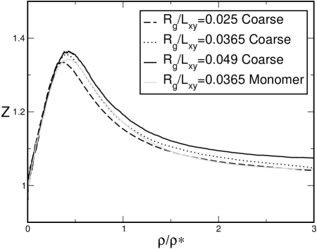
Figure 3: The equation-of-state $Z=\beta P/\rho$ for different box sizes, denoted by $R_{g}/L_{XY}$, calculated by coarse grained simulations and compared, at $R_{g}/L_{XY}=0.0365$, to an equivalent fully resolved monomer-level simulation

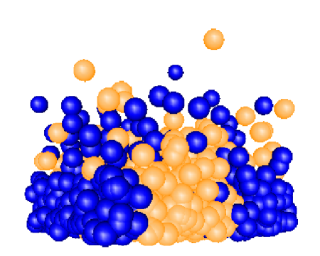
Figure 4: Snapshot of a configuration for $N_{A}=N_{B}=800$ polymers, showing the CM of each as a sphere of radius $R_{g}$. The sedimentation lengths are $\zeta_{A}=\zeta_{B}=2.11R_{g}$, and the open box has a base of length $L_{X}=L_{Y}=200$. Note that the existence of two interfaces is due to the use of periodic boundary conditions in the x and y directions.

The resulting equation-of-state $Z=P/\rho k_{B}T$ is plotted in figure 3. After an initial linear increase, $Z$ goes through a maximum around $\rho/\rho^{*}\lesssim 0.5$, before decreasing and apparently saturating at a value above one at high densities. This unusual behaviour may be traced back to to the phase separation, which is evident in the snapshot of a typical configuration shown in fig 4, and which will be analysed in more detail in section 5. The existence of phase boundaries leads one to expect a substantial dependence of the measured equation-of-state on the size of the simulation box.

To illustrate this size dependence, we have carried out MC simulations of the coarse-grained representation of the ISI model, based on the effective potential $v_{AB}(r)$ introduced in section 3 (fig 1) for three values of the ratio $R_{g}/(L_{XY})$ (where $L_{XY}=L_{X}=L_{Y}$ is the length of the square base of the simulation cell). These were carried out for $N_{A}=N_{B}=800-2000$ coarse-grained particles, with a sedimentation length $\zeta=2R_{g}$. Such simulations are typically two orders of magnitude faster than those based on the full monomer-level ISI model for the same number of polymers. For $R_{g}/(L_{XY})=0.0365$, the agreement between the equations of state calculated with the two representations is seen to be satisfactory in figure 3. The small discrepancies are probably due to the fact that we have neglected the density dependence of the effective potential $v_{AB}(r)$, for which we have used the zero density result shown in figure 1. The simulation data for the coarse-grained model plotted in figure 3 clearly illustrate the size dependence at high densities, i.e. in the region of phase coexistence. This is expected since the smaller the system, the larger the interfacial contribution to the equation-of-state; the former will become negligible only in the thermodynamic limit ($R_{g}/(L_{XY})\rightarrow 0$).

V Interpretation of the simulation data

The equation-of-state data of figure 3 can be understood in terms of an underlying phase separation, as suggested by fig 4. The phase diagram of the ISI model can be calculated, at least approximately, from the virial expansion of the free energy. The free energy per unit volume can be expanded as:

$$f=\frac{F}{Vk_{B}T}=f_{A}^{id}+f_{B}^{id}+2x(1-x)B_{AB}\rho^{2}+{\cal O}(\rho^{3})$$ (9)

where $f^{id}_{\alpha}=\rho_{\alpha}(ln(\Lambda_{\alpha}^{3}\rho_{\alpha})-1)$ and $B_{AB}$ is the second virial coefficient of equation (8). Differentiation of (9) with respect to $\rho$ yields:

$$Z=\frac{P}{\rho k_{B}T}=df/d\rho-f/\rho=1+2x(1-x)B_{AB}\rho+{\cal O}(\rho^{2}).$$ (10)

Above a critical density $\rho_{c}$, the free energy (9) leads to phase separation; by symmetry the critical concentration $c_{c}=1/2$, while $\rho_{c}=1/B_{AB}$. Inserting the numerical value $B_{AB}=9.5R_{g}^{3}$ reported in section 3, one finds $\rho_{c}/\rho^{*}=0.44$. Following an analysis similar to one presented in ref. louis one can calculate the spinodal curve analytically:

$$\rho_{s}(x)=\frac{1}{2B_{AB}\sqrt{x(1-x)}}.$$ (11)

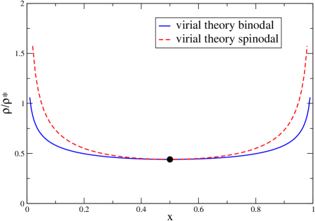
Figure 5: Spinodal and binodal demixing lines for the ISI model, calculated from second virial coefficient expansion of the free energy described in Eqs. 9 - 11.

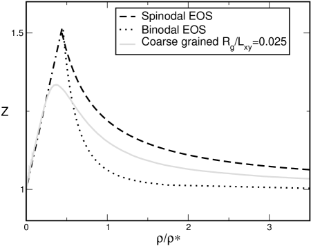
Figure 6: The equation-of-state from the largest coarse-grained system simulations is compared to theoretical curves, calculated from the binodal and the spinodal lines of a second virial expansion of the free energy described in Eqs. 9 - 11.

The binodal is easily calculated numerically, and results are summarised in figure 5; segregation of the two species is seen to be nearly complete for $\rho/\rho^{*}\sim 1$. The equation-of-state data of figure 3 may now be “read” as follows. As the altitude $z$ decreases in the polymer sediment, the local density $\rho(z)$ increases (c.f. figure 2). Up to $\rho/\rho^{*}\lesssim 0.4$ the system remains in the one phase region of the phase diagram in figure 5, and the equation-of-state Z increases linearity with $\rho/\rho^{*}$ according to (10); the slope of the linear portion of the MC-generated equation-of-state agrees well with that predicted by (10) (with $B_{AB}\simeq 9.5R_{g}^{3}$). When the local density $\rho(z)$ increases beyond the critical density $\rho_{c}/\rho^{*}\simeq 0.44$, the system enters the phase-coexistence region bounded by the binodal curve and separates symmetrically into two mixtures with compositions $x$ and $1-x$ which may be read from figure 5. The excess contribution to the pressure of the coexisting phases decreases with density, because the number of A-B contacts drops sharply in the A and B-rich phases as the overall density rises. At densities $\rho>\rho^{*}$, the nearly complete segregation means that coexisting phases behave practically as ideal cases of A or B polymers. Hence, for sufficiently large systems such that the interfacial contribution to the local stress is negligible compared to the bulk contributions, the equation-of-state $Z$ must return to its ideal gas value 1 for $\rho\gg\rho^{*}$.

The theoretical equation-of-state is compared in figure 6 to the MC data for the largest system. The agreement is seen to be only qualitative. The theoretical curve has a cusp point (rather than a rounded maximum) at the density where phase separation starts. In the simulations, the system may enter the metastable region comprised between the binodal and spinodal curves in figure 5. In that case the mixture may reach higher densities before segregating. The equation-of-state calculated on the assumption that the mixture separates into two phases along the spinodal curve is also shown in figure 6. It is gratifying to realise that the simulation data lie between the binodal and spinodal equations-of-state, which constitute two extreme limits of the actual scenario.

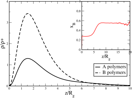
Figure 7: Density and concentration profiles $\rho_{A}(z)$, $\rho_{B}(z)$, $x(z)$ (inset) of a 70:30 mixture of ISI polymers.

In the more general case where the overall composition of the binary polymer solution $x\neq 0.5$ (i.e. $N_{A}\neq N_{B}$), the local concentration ratio, $x(z)$ will no longer be constant, and the extraction of $Z(\rho,x)$ from equation (5) requires several simulations of systems with different compositions. No attempt is made at a full investigation in the present paper, but the situation is illustrated in figure 7, where density and concentration profiles obtained from MC simulations of the full monomer description of a system with $N_{A}=480$ and $N_{B}=1120$ ($x=0.3$) polymers of $L_{A}=L_{B}=500$ in an open square based box of side length $L_{XY}=200$ are plotted. The concentration profile $x(z)$ is seen to vary substantially at altitudes where phase separation is expected to take place.

In this case, as well as for lower overall concentration fractions of A particles, we observe the formation of a vertical, cylindrical interface, rather than two planar interfaces as in figure 4. This observation can be understood as the consequence of a minimisation of the area over which unfavourable A-B contacts take place. Assuming that the distributions $\rho_{A}(z)$ and $\rho_{B}(z)$ of the two species are identical irrespective of the geometry of the interface, and that the height H of the two types of interfaces is the same, and noting that the radius r of the cylinder is related to the concentration $x$ by $x=\pi(r/L_{XY})^{2}$, one finds that the areas of the two planar and cylindrical interfaces are identical when $x=1/\pi$; below this value, the cylindrical interface will be preferred. We explicitly checked this by performing simulations for $N_{A}+N_{B}=1600$ polymers at $x=0.1,0.2,0.3,0.4$ and $0.5$. As expected, for the lowest three concentration ratios we find cylindrical interfaces, and for the two higher concentrations we find planar interfaces.

VI Conclusion

We have extended the sedimentation equilibrium method for the computation of the osmotic equation-of-state of polymer solutions to the case of binary polymer mixtures undergoing phase separation. The method was applied to the athermal ISI model, where polymer species A and B (assumed here to be of the same length) behave like ideal (random walk) polymers, but are mutually avoiding, i.e. monomers of different species cannot occupy the same lattice sites. This incompatibility leads to segregation for overall polymer densities higher than about one half of the overlap density $\rho^{*}$. This segregation leads to a somewhat unusual variation of the osmotic pressure with density, since outside the interfacial region, the mixture behaves as an ideal solution both in the low and high density limits.

The MC generated equation-of-state agrees well with the data obtained from a coarse-grained representation based on an effective interaction between the CMs of A-B pairs, and agrees semi-quantitatively with the predictions of a simple analytic theory based on a second virial expansion. The cusp in the equation-of-state predicted by the latter is rounded into a maximum in the MC data due to finite size effects. The present investigation suggests that the phase behaviour of segregating mixtures can be extracted from a measurement of the density profile of the inhomogeneous mixture in an external field. Although our model is highly oversimplified, we have demonstrated that our coarse-graining strategy can be applied in a straight-forward fashion to the demixing of polymer solutions. We plan to extend this methodology to more realistic polymer models, and to grand canonical ensemble simulations.

- (1) see e.g. M. Rubinstein and R.H. Colby, “Polymer Physics”, (Oxford University Press, 2003)
- (2) D. Broseta, L.Leibler and J.F. Joanny, Macromolecules 20, 1935 (1987)
- (3) A. Sariban and K. Binder, Colloid and Polymer Science 272, 1474 (1994)
- (4) B. Widom and J.S. Rowlinson, J.Chem.Phys. 52, 1670 (1970)
- (5) C.I. Addison, J.-P. Hansen and A.A. Louis, Chem.Phys.Chem. (in press 2005); cond-mat/0411319
- (6) C.I. Addison, J.-P. Hansen, V. Krakoviack and A.A. Louis, Mol.Phys. (in press 2005); cond-mat/0507360
- (7) T. Biben, J.-P. Hansen and J.L. Barrat, J.Chem.Phys. 98, 7330 (1993)
- (8) M. Schmidt, M. Dijkstra and J.-P. Hansen, Phys. Rev. Lett. 93, 088303 (2004); J.Phys.Condens.Matter 16, 4185 (2004)
- (9) J. Dautenhahn and C.K. Hall, Macromolecules 27, 5399 (1994)
- (10) P.G. Bolhuis, A.A. Louis, J.-P. Hansen and E.J. Meijer J.Chem.Phys. 114, 4296 (2001)
- (11) P.G. Bolhuis and A.A. Louis, Macromolecules 35, 1860 (2002)
- (12) C. Mayer, C. N. Likos, and H. Löwen, Phys. Rev. E 70, 041402 (2004).
- (13) S.O. Nielsen, C.F. Lopez, G. Srinivas and M.L. Klein, J. Phys.: Condens. Matter 16, R481 (2004).
- (14) A. Pelissetto and J.-P. Hansen, J.Chem.Phys. 112, 134904 (2005)
- (15) A.A. Louis, P.G. Bolhuis and J.-P. Hansen, Phys.Rev.E 62, 7961 (2000)